Laser Rangefinder

Group 2

Aaron Smeenk

Jackson Ritchey

Keith Hargett

Kourtney Bosshardt

Table of Contents 1. Introduction

1.1. Executive Summary 1.2. Motivation and Goals 1.3. Specifications 1.4. Design Constraints and Standards

1.4.1. Economic 1.4.2. Environmental

1.4.2.1. Outdoors/indoors 1.4.3. Health and Safety

1.4.3.1. Lithium-Ion Batteries 1.4.3.2. Lasers

2. Research

2.1. Similar Projects/LIDAR Technologies 2.1.1. Instructables Project 2.1.2. Webcam Based DIY Laser Rangefinder 2.1.3. OSLRF-01

2.1.3.1. Transmitter End 2.1.3.2. Receiver End 2.1.3.3. Control Logic

2.2. Control system 2.2.1. SLAM

2.3. Base Module 2.3.1. Interface

2.3.1.1. SPI 2.3.1.2. I2C 2.3.1.3. UART

2.3.2. Motor Technology 2.3.2.1. Servo Motors 2.3.2.2. Continuous Rotation Servo Motors 2.3.2.3. Brushed DC (BDC) Motors 2.3.2.4. Brushless DC (BLDC) Motors 2.3.2.5. Stepper Motors 2.3.2.6. Motor Encoders

2.3.2.6.1. Optical Rotary Encoders 2.3.2.6.2. Magnetic Rotary Encoders 2.3.2.6.3. Encoder Operation and Specifications

2.3.2.7. Motor Drivers 2.3.2.7.1. H-Bridges 2.3.2.7.2. Brushed DC Motor Drivers 2.3.2.7.3. Brushless DC Motor Drivers 2.3.2.7.4. Stepper Motor Drivers

2.3.2.8. Motor Gearboxes 2.3.3. Motor Control

2.4. Range Finding Device

2.4.1. Interface 2.4.2. Optics 2.4.3. Design Approaches

2.4.3.1. Laser Time of Flight (Digital) 2.4.3.2. Laser Interferometry 2.4.3.3. Laser Phase Shift 2.4.3.4. Pulse Amplitude

2.5. Power Management 2.5.1. Battery Technologies

2.5.1.1. Lithium-Ion 2.5.1.2. Lithium-Polymer

2.5.2. Power Control 2.5.2.1. Linear Regulators

2.5.2.1.1. Simple Shunt Regulators 2.5.2.1.2. Simple Series Regulators

2.5.2.2. Switching Regulators 2.5.2.2.1. Buck Regulator 2.5.2.2.2. Boost Regulator

2.5.2.3. Battery Monitoring 2.5.2.3.1. Safety Procedures for Li-Po Batteries 2.5.2.3.2. Charge Controllers

2.5.2.3.2.1. Simple Charge Controllers 2.5.2.3.2.2. Complex Charge Controllers

2.5.2.3.3. Protection Circuits 2.5.2.3.4. Temperature sensors 2.5.2.3.5. Over-voltage control 2.5.2.3.6. Under-voltage control

2.5.2.4. Power Monitoring (INA219) 2.7. Data Interpretation Software 2.7.1 Point Cloud 2.7.2 Computer Vision

3. Design 3.1. Block Diagram 3.2. Base Module

3.2.1. Interfacing with the Base Module 3.2.2. Mechanical 3.2.3. Electrical

3.2.3.1. Microcontroller 3.2.4. Software

3.3. Range Finder 3.3.1. Interfacing with the Range Finding Module 3.3.2. Electrical

3.3.2.1. TDC7200 3.3.2.2. Microcontroller

3.3.2.2.1. ARM Cortex m4 3.3.2.2.1.1. STM32F407

3.3.2.2.1.2. STM32F427 3.3.2.2.2. PSOC5 3.3.2.2.3. ATMEGA328p

3.3.3. Optics 3.3.3.1. Transmitter

3.3.3.1.1. SPL-PL90 Laser Diode 3.3.3.1.2. Laser Driver

3.3.3.2. Receiver 3.3.3.2.1. SFH2701 Photodiode 3.3.3.2.2. Amplifier

3.3.4. Software 3.4. Power Consumption 3.5. Software Configuration

3.5.1. Dynamic Changes 3.5.2. Demonstration Software

3.5.2.1. Native Data Visualizer 3.5.2.2. Web Client 3.5.2.3. Android App

3.6. System Schematics 3.6.1. Base Module 3.6.2. Range Finder

4. Build 4.1. Parts 4.2. Bill of Materials

5. Test 5.1. Instructables Rangefinder 5.2. Base Module

5.2.1. Motor 5.2.2. Microcontroller

5.3. Rangefinder Module 5.4. Software

6. Administrative Content 6.1. Milestone

6.1.1. June 6.1.2. July 6.1.3. August 6.1.4. September 6.1.5. October 6.1.6. November

6.2. Budget 6.3. Version Control

7. Conclusion 8. Bibliography

A. Copyright Permissions

Table of Figures Figure 1 Webcam DIY Laser Rangefinder Calculation Diagram Figure 2 Block Diagram of Functions of the OSLRF-01 Figure 3 Timing Diagram of the Signals in the OSLRF-01 Figure 4 Connection Diagram of the OSLRF-01 Figure 5 Outgoing Laser Pulse Timebase Expander and Buffer Schematic Figure 6 Schematic of Receiver End of Optics Figure 7 Schematic of the Control Logic of the Optics Figure 8 Block Diagram of the SLAM Process Figure 9 Diagram of Lorentz Force Figure 10 Diagram of Brushless DC Motors Figure 11 H-Bridge Motor Control Design Figure 12 H-Bridge Motor Control Operation Figure 13 Range Finding Module Laser Front End Figure 14 Optical Behavior of Device Figure 15 Effect of Specular Reflection at Different Angles Figure 16 Simplified Laser Pulse and Detection Circuit Figure 17 Time Of Flight Measure Circuit Figure 18 Effect of Rise Time on Accuracy Figure 19 Active Mode-locked Laser Diagram Figure 20 Passive Mode-locked Laser Diagram Figure 21 Pulse Generation of Mode-locking Laser Figure 22 Phase Shift Rangefinder Block Diagram Figure 23 Battery Technology Comparison Figure 24 Nominal Voltage vs Discharge - Lithium-Polymer Figure 25 Nominal Voltage vs Time - Lithium-Polymer Figure 26 Simple Shunt Regulator Circuit Figure 27 Simple Series Regulator Circuit Figure 28 Buck Regulator Circuit Figure 29 Boost Regulator Circuit Figure 30 Rangefinder High Level Design Figure 31 Block Diagram of Entire System Figure 32 Command Protocol Flow Chart Figure 33 Mechanical Design Figure 34 Software Design Architecture of Base Module Figure 35 Measurement deviation VS clock period Figure 36 Clock Jitter Figure 37 Standard Deviation vs Time of Flight Figure 38 Measuring Mode 1 Figure 39 Time of flight equation Figure 40 Laser Driver Figure 41 Laser Receiver Figure 42 Software Design Architecture of Laser Rangefinder Module Figure 43 Demonstration Software Data Flow Figure 44 Base Module Top Level Figure 45 Base Module Microprocessor

Figure 46 Base Module Microprocessor Power Figure 47 Base Module System Power Figure 48 Rangefinder Module Top Level Figure 49 Rangefinder Microprocessor Figure 50 Rangefinder Microprocessor Power Figure 51 Laser Driver Schematic Figure 52 Laser Receiver Schematic Figure 53 Rangefinder System Power Table of Tables Table 1 Specifications of the OSLRF-01 Table 2 Average Expected Power Consumption of System Table 3 Base Module Connectors BOM Table 4 Base Module Capacitors BOM Table 5 Base Module Integrated Circuits BOM Table 6 Base Module Other BOM Table 7 Rangefinder Capacitors BOM Table 8 Rangefinder Capacitors pt2 BOM Table 9 Rangefinder Connectors BOM Table 10 Rangefinder Resistors BOM Table 11 Rangefinder Optics BOM Table 12 Rangefinder Integrated Circuits BOM Table 13 Rangefinder Other BOM Table 14 Timeline Table 15 Budget

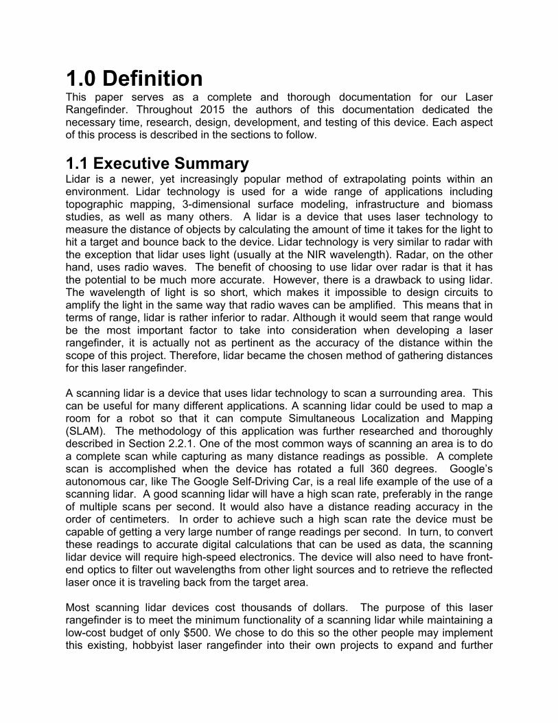
1.0 Definition This paper serves as a complete and thorough documentation for our Laser Rangefinder. Throughout 2015 the authors of this documentation dedicated the necessary time, research, design, development, and testing of this device. Each aspect of this process is described in the sections to follow. 1.1 Executive Summary Lidar is a newer, yet increasingly popular method of extrapolating points within an environment. Lidar technology is used for a wide range of applications including topographic mapping, 3-dimensional surface modeling, infrastructure and biomass studies, as well as many others. A lidar is a device that uses laser technology to measure the distance of objects by calculating the amount of time it takes for the light to hit a target and bounce back to the device. Lidar technology is very similar to radar with the exception that lidar uses light (usually at the NIR wavelength). Radar, on the other hand, uses radio waves. The benefit of choosing to use lidar over radar is that it has the potential to be much more accurate. However, there is a drawback to using lidar. The wavelength of light is so short, which makes it impossible to design circuits to amplify the light in the same way that radio waves can be amplified. This means that in terms of range, lidar is rather inferior to radar. Although it would seem that range would be the most important factor to take into consideration when developing a laser rangefinder, it is actually not as pertinent as the accuracy of the distance within the scope of this project. Therefore, lidar became the chosen method of gathering distances for this laser rangefinder. A scanning lidar is a device that uses lidar technology to scan a surrounding area. This can be useful for many different applications. A scanning lidar could be used to map a room for a robot so that it can compute Simultaneous Localization and Mapping (SLAM). The methodology of this application was further researched and thoroughly described in Section 2.2.1. One of the most common ways of scanning an area is to do a complete scan while capturing as many distance readings as possible. A complete scan is accomplished when the device has rotated a full 360 degrees. Google’s autonomous car, like The Google Self-Driving Car, is a real life example of the use of a scanning lidar. A good scanning lidar will have a high scan rate, preferably in the range of multiple scans per second. It would also have a distance reading accuracy in the order of centimeters. In order to achieve such a high scan rate the device must be capable of getting a very large number of range readings per second. In turn, to convert these readings to accurate digital calculations that can be used as data, the scanning lidar device will require high-speed electronics. The device will also need to have front-end optics to filter out wavelengths from other light sources and to retrieve the reflected laser once it is traveling back from the target area. Most scanning lidar devices cost thousands of dollars. The purpose of this laser rangefinder is to meet the minimum functionality of a scanning lidar while maintaining a low-cost budget of only $500. We chose to do this so the other people may implement this existing, hobbyist laser rangefinder into their own projects to expand and further

develop its functionalities. This can be accomplished in several different ways including exchanging the optics we decided to use with more expensive optics, using the gathered data to visualize environments in 3D, or by adding a navigation system to maneuver around obstacles in a room. To allow for demonstration of this laser rangefinder, we developed a collection of software modules that interface nicely with the hardware of the device. This software is used to provide a real-time visual representation of the data being gathered by the laser rangefinder as it is scanning its surroundings area. The software we implement can be accessed from any device and serves as a minimal, yet thorough presentable illustration of lidar technology. 1.2 Motivation and Goals As a group we recognize that autonomous motion is an extremely hot topic these days. Self-driving cars are becoming increasingly popular as the technology supporting them advances. We all believe that the best way to improve technology is to get more minds working on it. The price and availability of good optical technology, such as lasers and photodiodes, has come down into an affordable price range for the average consumer as optic research has increased. Lidar technology, however, has not. Outside of cheap IR LED and sonar rangefinders the typical hobbyist interested in the field has almost no options unless they can afford to spend a few thousand dollars. We firmly trust that the technology and resources are available, but that a good solution has not hit the market yet. The goal of this project is to design a true lidar/range-finding system that would only cost in a few hundred dollars rather than upmost thousands of dollars. The specific goals for this laser rangefinder are as follows: ● To serve as an accurate range-finding system. ● To contain a reliable and complete package, including optics, electronics, and

moving parts. ● To maintain a simplistic interface. ● To be able to display functioning capabilities of a lidar system in action.

1.3 Specifications When designing a lidar system, there are many specifications to take into consideration. The specifications discussed here are by no means limited in regards to all of the factors of a lidar system, but instead represent some of the most important design considerations that were taken into account when designing this laser rangefinder. All of these specifications have directly affected the accuracy and functionality of this laser rangefinder. Physically, we wanted to design a portable device that was small in size. We initially decided that a maximum weight of five pounds and an occupational area of 3 meters would satisfy the needs of our device. These dimensions would still maintain an accurate and thorough design outcome. We also wanted to be able to gather the data through a by connecting a computer or device to the laser rangefinder through a USB port. In order to allow for different devices and computers to connect to the device, we

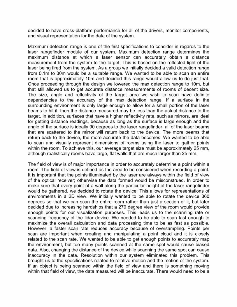
decided to have cross-platform performance for all of the drivers, monitor components, and visual representation for the data of the system. Maximum detection range is one of the first specifications to consider in regards to the laser rangefinder module of our system. Maximum detection range determines the maximum distance at which a laser sensor can accurately obtain a distance measurement from the system to the target. This is based on the reflected light of the laser being fired from the system. As a group we initially decided a valid detection range from 0.1m to 30m would be a suitable range. We wanted to be able to scan an entire room that is approximately 10m and decided this range would allow us to do just that. Once proceeding through the design we lowered the max detection range to 10m, but that still allowed us to get accurate distance measurements of rooms of decent size. The size, angle and reflectivity of the target area we wish to scan have definite dependencies to the accuracy of the max detection range. If a surface in the surrounding environment is only large enough to allow for a small portion of the laser beams to hit it, then the distance measured may be less than the actual distance to the target. In addition, surfaces that have a higher reflectivity rate, such as mirrors, are ideal for getting distance readings, because as long as the surface is large enough and the angle of the surface is ideally 90 degrees to the laser rangefinder, all of the laser beams that are scattered to the mirror will return back to the device. The more beams that return back to the device, the more accurate the data becomes. We wanted to be able to scan and visually represent dimensions of rooms using the laser to gather points within the room. To achieve this, our average target size must be approximately 25 mm, although realistically rooms have large, flat walls that are much larger than 25 mm. The field of view is of major importance in order to accurately determine a point within a room. The field of view is defined as the area to be considered when recording a point. It is important that the points illuminated by the laser are always within the field of view of the optical receiver; otherwise the data formed would be misconstrued. In order to make sure that every point of a wall along the particular height of the laser rangefinder would be gathered, we decided to rotate the device. This allows for representations of environments in a 2D view. We initially wanted to be able to rotate the device 360 degrees so that we can scan the entire room rather than just a section of it, but later decided due to increasing hardships that a 270 degree view of the room would provide enough points for our visualization purposes. This leads us to the scanning rate or scanning frequency of the lidar device. We needed to be able to scan fast enough to maximize the overall calculation and data processing time to be as fast as possible. However, a faster scan rate reduces accuracy because of oversampling. Points per scan are important when creating and manipulating a point cloud and it is closely related to the scan rate. We wanted to be able to get enough points to accurately map the environment, but too many points scanned at the same spot would cause biased data. Also, changing the distance of the device while scanning the same spot can cause inaccuracy in the data. Resolution within our system eliminated this problem. This brought us to the specifications related to relative motion and the motion of the system. If an object is being scanned within the field of view and there is something moving within that field of view, the data measured will be inaccurate. There would need to be a

way to determine whether the movement has skewed the data and if so there would need to be at least one way to fix this problem. How we decided to eliminate this problem is by putting a time of life on the points scanned. Say the time of life of a point scanned is 10 seconds and the device is currently scanning a spot in the room where a person is walking past. Then, the points that go away after the person is no longer in the scanning view will not be included in the representation of the room 10 seconds after the person has left the field of view. This was of huge importance on the software aspect of the design to be able to determine which points scanned are accurate representations of points in the room and which point are erroneous and need to be discarded. Motion of the system also was also considered in the first stages of specifying the laser rangefinder. If we had chosen for out system to not be stationary, there would need to be a way to determine if the same spot is being scanned even though the distance away from that spot has increased or decreased. This would rely heavily on software implementation to determine if the same spot is in fact being measured, regardless of the distance from that spot, and could be easily implemented in further applications of this device. For this laser rangefinder, there are two power requirements that must be addressed. The first is the laser power. An increase in the maximum range is proportional to the square root of the laser power, so the laser power needed for this device is dependent on the maximum distance we decided upon. The second power to be considered is the power for the overall system. The power will run on a single rail system and will consume approximately 30 W. The rangefinder board contains regulation mechanisms for all of the components on the board. It also has ways of monitoring the overall voltage on each board and comparing different inputs for power regulation. 1.4 Design Constraints and Standards With unlimited resources and funds anyone could create anything. However in reality and specifically within the scope of this project that was not the case. Throughout the design phase and even within defining our project, we needed to consider several constraints that limited the potential of our design. The types of these constraints include, but are not limited to economic, environmental, and health and safety. Some of these constraints may be due to accepted standards, for example consider health and safety constraints. 1.4.1 Economic The economic constraint of this project is by far the most concerning and pertinent limitation to the design of our lidar system. Every single financial aspect of this project has been paid for by us or has been taken care of through personal resources. Most laser range finders on the market that can perform to our expectations cost, at minimum, a couple hundred dollars. Considering we are all broke college kids, we need to design a laser range finder and a base module that does not cost more than $400.

1.4.2 Environmental Environmental constraints pertain to how the physical environment will affect the design of our system. This includes whether the system is indoors or outdoors, in clear weather or in rain as well as many other factors. We need our system to operate indoors, at normal room temperature. We could also define our system to work outside which would not affect any of the constraints we have already discussed. 1.4.3 Health and Safety The main concern in regards to health and safety is the laser. The potential risk is that if the laser is too powerful it may damage people’s eyes if they look directly at the device. This is problematic because the device is intended to be use in areas that may have a lot of people. In order to ensure the safety of the public during testing and operating this device, the follow standards were followed; ANSI Z136, IEC 60825. These standards define 4 classes of laser based on their power and wavelength. The class of laser that is considered safe is class 1 lasers. 1.4.3.1 Lithium-Ion Batteries Since the widespread commercial use of lithium-ion batteries began, there has been a variety of lithium-ion designs that have been developed to meet a wide variety of product demands. Choosing the right battery for any application includes considering the power and energy requirements of that application, the environment in which the battery-powered product will be used and the battery cost. Health and safety concerns of lithium-ion batteries are documented and researched so that they can have practical use. Lithium-ion batteries are required to include a mandatory protection circuit to ensure safety under all circumstances. An external electronic protection circuit prevents the charge voltage of any cell within the battery from exceeding 4.30V. Prevention from overheating includes a fuse that cuts the current if the skin temperature of any cell gets close to 90�. Also, over-discharging of the battery is averted through the use of a control circuit that cuts off the current path once it approaches 2.20V/cell. Although these safeguards are implemented in single and multi-cell batteries, there are still performance and safety issues that exist. These include the thermal stability of active materials within the battery at high temperatures and the occurrence of internal short circuits that may cause an increase in temperature that changes the conditions in a way that causes a further increase in temperature leading to destructive results. Product standards and testing protocol have been developed to address some of these safety risks. These standards include, but are not limited to the following: the UL 1642: Lithium Batteries by Underwriters Laboratories; Recommendations on the Transport of Dangerous Good, Manual of Tests and Criteria, Part III, Section 38.3 by the United Nations; and IEC 62133: Secondary Cells and Batteries Containing Alkaline or Other Non-acid Electrolytes — Safety Requirements for Portable Sealed Secondary Cells, and for Batteries Made from Them, for Use in Portable Applications by the International Electrotechnical Commision.

1.4.3.2 Lasers There are always constraints in regards to health and safety whenever dealing with lasers. If lasers are not fired within a specific wavelength spectrum, it could cause serious radiation and other physical damage to its surroundings. Government regulations limit the safety and usage of lasers due to the simple fact that even relatively small amounts of laser light can cause permanent eye damage. Lasers are classified by wavelength and maximum output power into four classes. This classification system is part of the revised IEC 60825 standard and is also incorporated into the US-oriented ANSI Laser Safety Standard (ANSI Z136.1). The U.S. Food and Drug Administration accepts this system on all laser products imported into the U.S. Within the optical design of our laser range finder, we will narrow the beam of our laser to increase the accuracy of distance measurements. This means that the highest level laser we will use is a Class 1M laser, which is the second lowest laser class.

2.0 Research The major area for research of the laser rangefinder was concerned with the rangefinder module. This research was focused on process of operations, optics, and high-speed electronics. Further research for the base module was focused on different motor technologies and motor encoders. 2.1 Similar projects and lidar technologies In an effort to get a greater understanding of our project as well as lidar in general, we first began by looking at similar projects to find potential reference designs. This helped us get a better understand of the underlying technology that was actually utilized within our own project. 2.1.1 Instructables Project We recreated the instructables project, Homemade Infrared Rangefinder by Pyrohaz, to serve as a quick prototype in an effort to gain an understanding of some of the processes to be taken as a whole [5]. The instructables project being utilized describes an IR rangefinder placed on top of a servo to act as an “IR rader”. The original project then displayed this recovered data to a radar type plot on a screen. We, as a group may not intend to utilize an IR range finder in the final prototype, however, this small project will allow us to see how lidar works first hand as well as potentially receive some preliminary data to begin pointcloud manipulations on in order to determine the final library and processes desired to perform these manipulations for our final presentation. This first, quick prototype also gave us a chance to experiment in PCB design as well as the ability to gain experience prior to designing our final working prototype in an effort to attempt to foresee potential issues in the board design process as well as work out bugs for when cutting a board from an in house machine rather than sending the board to a professional board house.

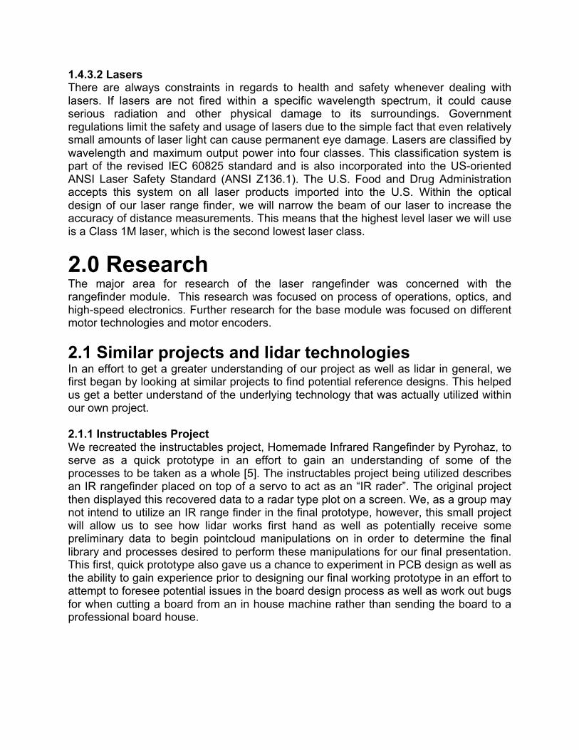
2.1.2 Webcam Based DIY Laser Rangefinder This project, developed by Todd Danko, shows how a laser rangefinder can be constructed using a mini laser pointer, a webcam and a single piece of cardboard. The mini laser pointer is configured alongside a single camera to provide mono-machine vision with range information. Its purpose is to provide laser distance measurements to machine vision applications such as obstacle identification and avoidance. First the laser-beam is projected onto the target within the field of view of the camera. Figure 1 below shows that if this is done correctly, this beam is parallel to the optical axis of the camera. The camera then takes a picture of the scene, which includes the point of the laser on the target. The image is then sent to a computer where algorithms run to determine the position of the point of the laser within the scene. The distance range to the object is calculated by determining where along the y-axis of the image the laser point falls. If the laser dot is closer to the center of the image, the target is farther away from the source. Figure 1 also shows how the distance is calculated.

(Permission For Use by Todd Danko)

Figure 1 Webcam DIY Laser Rangefinder Calculation Diagram

Although this project is a good representation of how to use a laser to perform distance calculations, we did not like the idea of using a camera to capture the scene. We want to be able to map the scene based on the distance points we measure from our laser rangefinder. All in all, this was a good introduction to laser rangefinding. 2.1.3 OSLRF-01 The OSLRF-01 is an open source time-of-flight sensor that configures the front end of a laser rangefinder. Once power is applied to it, it independently calculates the time it takes for a laser pulse to travel from the device, to the surface being scanned and back to the device by analyzing the electrical signals it produces. This open source project was extremely insightful and provided us with a significant amount of consideration when determining parts for our own design. Based on this project, we decided to use the same transimpedance amplifier chip, the lens for both the transmitting and receiving sides, and the laser driver that were used in this OSLRF-01 project.

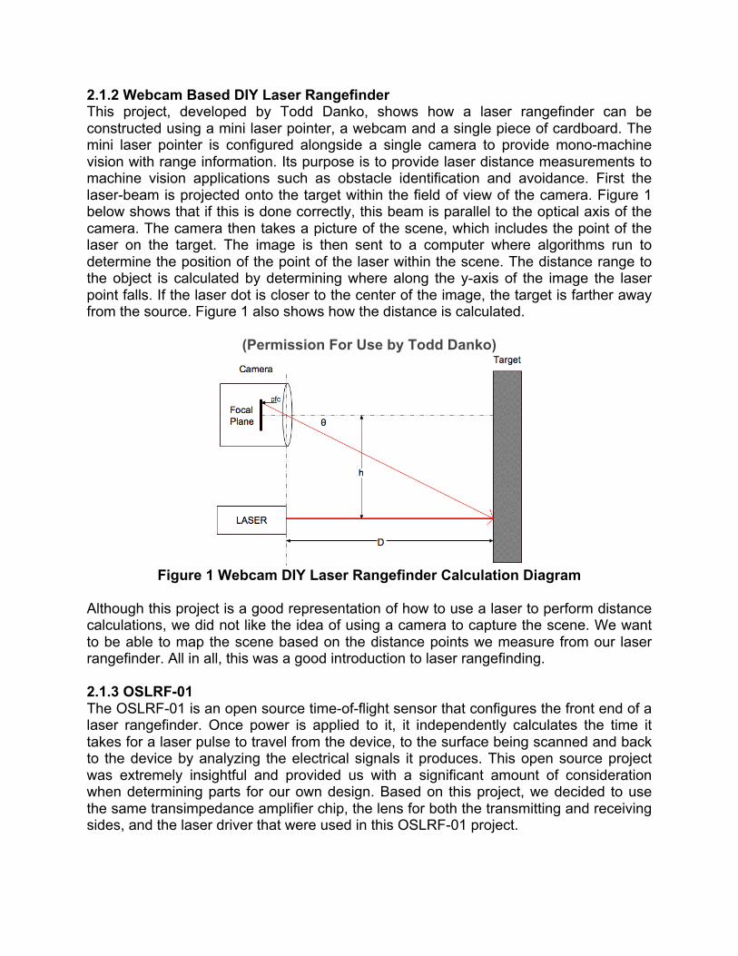
The OSLRF-01 is made up of a laser, a photodiode, optics, amplifiers, and sequential-equivalent-time-sampling circuits. Together these components create the signals needed to calculate the distance. These signals are then amplified and slowed down, which allows them to be analyzed on a manageable time scale. The signals outputted from the OSLRF-01 are the outgoing laser pulse, the return signal, and several means of obtaining time values. The OSLRF-01 does not actually convert the signals into distance measurements, but it is made so that it can easily integrated into a system that can perform those calculations. The OSLRF-01 functions as follows. First the control logic fires the laser and then the sequential-equivalent-time-sampling circuits sample the outgoing laser pulse. This operates to slow the signal down to a more justifiable time scale. The slowed down signal is outputted on the “Zero” pin of the OSLRF-01’s PCB. The lens is used to collimate the optical output of the laser into smaller beams which is then projected onto the surface in front of the device through the laser flash. Once the laser leaves the transmitting lens, it travels at the speed of light to the target surface and reflects back to the receiver lens. The receiver lens focuses the laser light onto a SFH2701 photodiode. This photodiode creates a brief current pulse that travels through a transimpedance amplifier (TIA) so that the pulse is amplified. Once the transimpedance amplifier turns the signal into a voltage, the voltage goes through sequential-equivalent-time-sampling circuits to create a slowed down version of the return signal. Finally, the slowed down signal gets amplified and is outputted on the “Return” pin of the OSLRF-01’s PCB. Below, in Figure 2, shows a block diagram of the functions of the OSLRF-01.

Figure 2 Block Diagram of Functions of the OSLRF-01

Timing the signal is a critical function in regards to the accuracy of the distance measurements obtained from the signal of the laser. The OSLRF-01 uses a high frequency oscilloscope to see real-time signals that pass through a sequential-equivalent-time-sampling circuit. This circuit slows down the signal so that the ADC inputs of a microcontroller can capture them. The signals are slowed down 100,000 times the original signals and are used by an expanded time base generator to produce

the desired waveform of the signal. The amount of expansion can be adjusted to modify the scan rate and resolution of the distance measurements. The importance of the ability to adjust this setting is discussed in more detail further along this section. The OSLRF-01 uses a timer with a 122 ns real-time span. This is equivalent to a distance measurement of 18.33 m at the speed of light to the target. Once the sequential-equivalent-time-sampling circuit expands the timebase, the span will be stretched out to over 20 ms. It can also be adjusted to span to over one second. Regardless of the duration of the span, the distance will always be equivalent to 18.33m. The expanded timebase uses a Sync signal to indicate the start and end of a measurement. A new measurement begins at the falling edge of the Sync square wave and ends at the next falling edge, which is also the beginning of a new measurement, because the measurements are taken continuously. The distance to any signal on the extended timebase is a proportion of the period of the Sync signal which is always 18.33 m. The Control voltage input can change the period of the Sync signal by modifying the timing of the sequential-equivalent-time-sampling circuit creating either a faster or slower expanded timebase. The sequential-equivalent-time-sampling circuit performs the same timebase expansion on the pulse signal from the Zero output, the signal on the Return output and the Sync signal. The signal to fire the laser on the expanded timebase is supposed to occur at the exact same time as the falling edge of the Sync signal, but there is a time delay before the laser actually produces the light. This delay is about 10 ns in real-time and it is the difference in time between the falling edge of the Sync signal and when the laser pulse is seen on the Zero output. Signals also have width that takes up some of the available measuring range. These two bounds limit the entire 18.33 m of the timing range from being available for the distance measurements. In order to accurately measure the distance to the target the firing delay of the laser pulse on the Zero output pin must be taken into account. This is done by first measure the period between two consecutive falling edges of the Sync signal (Sp), then measuring the time from falling edge of the Sync signal to the Zero signal (Zt), and finally measuring the the time from the falling edge of the Sync signal to the Return signal (Rt). Once these measurements are obtained, the distance (d) can be calculated as follows:

d = ((Rt - Zt) / Sp ) * 18.33 m There is also a Convert signal that is synchronous with the sequential-equivalent-time-sampling circuit that will reduce the noise within the returning signals. It does this by triggering successive ADC conversions from the connected microcontroller and comparing them with an ADC conversion at a different rate. This timing concept is better realized below in Figure 3.

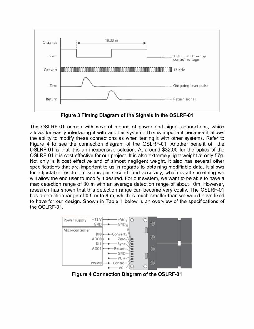
Figure 3 Timing Diagram of the Signals in the OSLRF-01

The OSLRF-01 comes with several means of power and signal connections, which allows for easily interfacing it with another system. This is important because it allows the ability to modify these connections as when testing it with other systems. Refer to Figure 4 to see the connection diagram of the OSLRF-01. Another benefit of the OSLRF-01 is that it is an inexpensive solution. At around $32.00 for the optics of the OSLRF-01 it is cost effective for our project. It is also extremely light-weight at only 57g. Not only is it cost effective and of almost negligent weight, it also has several other specifications that are important to us in regards to obtaining modifiable data. It allows for adjustable resolution, scans per second, and accuracy, which is all something we will allow the end user to modify if desired. For our system, we want to be able to have a max detection range of 30 m with an average detection range of about 10m. However, research has shown that this detection range can become very costly. The OSLRF-01 has a detection range of 0.5 m to 9 m, which is much smaller than we would have liked to have for our design. Shown in Table 1 below is an overview of the specifications of the OSLRF-01.

Figure 4 Connection Diagram of the OSLRF-01

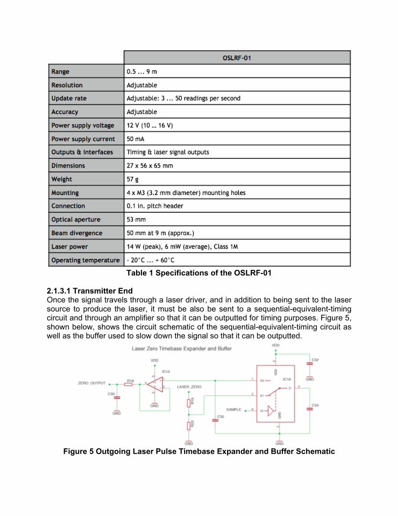
Table 1 Specifications of the OSLRF-01

2.1.3.1 Transmitter End Once the signal travels through a laser driver, and in addition to being sent to the laser source to produce the laser, it must be also be sent to a sequential-equivalent-timing circuit and through an amplifier so that it can be outputted for timing purposes. Figure 5, shown below, shows the circuit schematic of the sequential-equivalent-timing circuit as well as the buffer used to slow down the signal so that it can be outputted.

Figure 5 Outgoing Laser Pulse Timebase Expander and Buffer Schematic

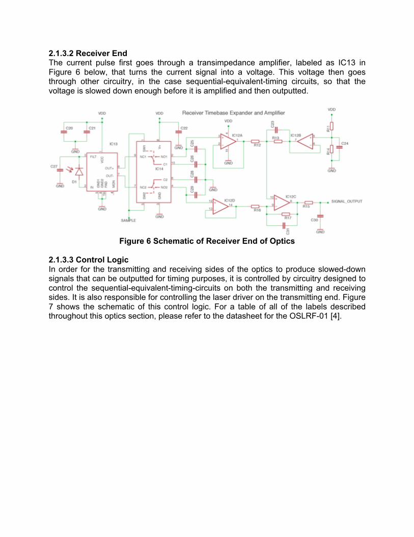
2.1.3.2 Receiver End The current pulse first goes through a transimpedance amplifier, labeled as IC13 in Figure 6 below, that turns the current signal into a voltage. This voltage then goes through other circuitry, in the case sequential-equivalent-timing circuits, so that the voltage is slowed down enough before it is amplified and then outputted.

Figure 6 Schematic of Receiver End of Optics

2.1.3.3 Control Logic In order for the transmitting and receiving sides of the optics to produce slowed-down signals that can be outputted for timing purposes, it is controlled by circuitry designed to control the sequential-equivalent-timing-circuits on both the transmitting and receiving sides. It is also responsible for controlling the laser driver on the transmitting end. Figure 7 shows the schematic of this control logic. For a table of all of the labels described throughout this optics section, please refer to the datasheet for the OSLRF-01 [4].

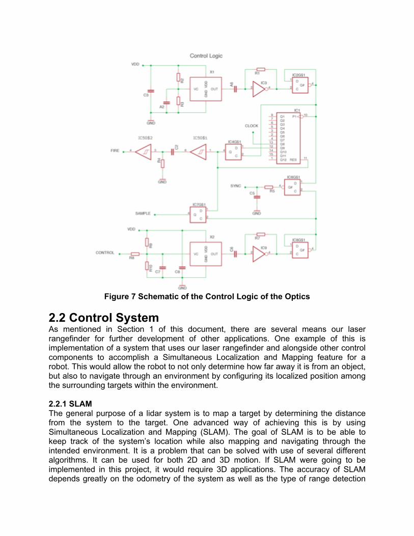
Figure 7 Schematic of the Control Logic of the Optics

2.2 Control System As mentioned in Section 1 of this document, there are several means our laser rangefinder for further development of other applications. One example of this is implementation of a system that uses our laser rangefinder and alongside other control components to accomplish a Simultaneous Localization and Mapping feature for a robot. This would allow the robot to not only determine how far away it is from an object, but also to navigate through an environment by configuring its localized position among the surrounding targets within the environment. 2.2.1 SLAM The general purpose of a lidar system is to map a target by determining the distance from the system to the target. One advanced way of achieving this is by using Simultaneous Localization and Mapping (SLAM). The goal of SLAM is to be able to keep track of the system’s location while also mapping and navigating through the intended environment. It is a problem that can be solved with use of several different algorithms. It can be used for both 2D and 3D motion. If SLAM were going to be implemented in this project, it would require 3D applications. The accuracy of SLAM depends greatly on the odometry of the system as well as the type of range detection

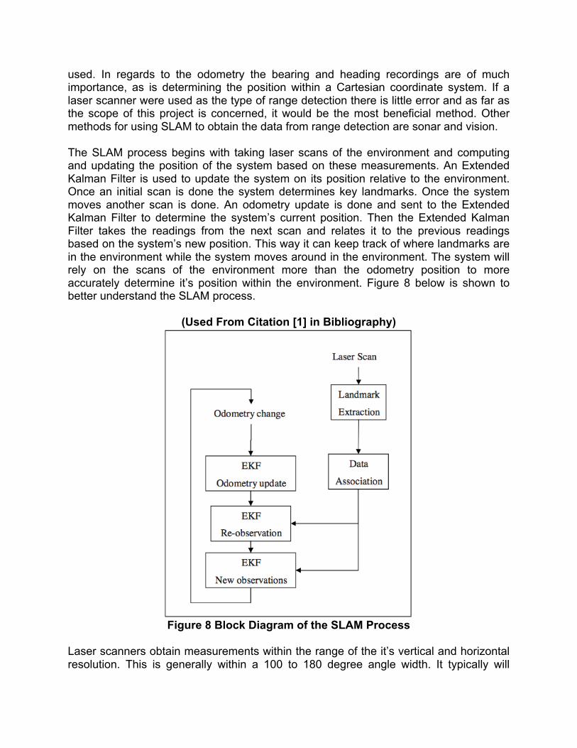
used. In regards to the odometry the bearing and heading recordings are of much importance, as is determining the position within a Cartesian coordinate system. If a laser scanner were used as the type of range detection there is little error and as far as the scope of this project is concerned, it would be the most beneficial method. Other methods for using SLAM to obtain the data from range detection are sonar and vision. The SLAM process begins with taking laser scans of the environment and computing and updating the position of the system based on these measurements. An Extended Kalman Filter is used to update the system on its position relative to the environment. Once an initial scan is done the system determines key landmarks. Once the system moves another scan is done. An odometry update is done and sent to the Extended Kalman Filter to determine the system’s current position. Then the Extended Kalman Filter takes the readings from the next scan and relates it to the previous readings based on the system’s new position. This way it can keep track of where landmarks are in the environment while the system moves around in the environment. The system will rely on the scans of the environment more than the odometry position to more accurately determine it’s position within the environment. Figure 8 below is shown to better understand the SLAM process.

(Used From Citation [1] in Bibliography)

Figure 8 Block Diagram of the SLAM Process

Laser scanners obtain measurements within the range of the it’s vertical and horizontal resolution. This is generally within a 100 to 180 degree angle width. It typically will

obtain measurements every .25 to 1.0 degrees. The lengths determined at these angles are then outputted as length measurements using a serial port. If a length cannot be accurately measured, a higher threshold value is used to show that it is an error. The odometry measurements are important in determining the position of the system based on the movement of the system’s wheels. In order to accurately determine the position of the system and it’s surrounding environment the odometry data and data from the laser scans must be determined at the same time. It is necessary to be able to control the rate at which these measurements are formed. There are several ways to determine specific landmarks within an environment which is important in forming the environment itself as well as determining the system’s position in respect to these landmarks. The method that would be used in this project is Random Sampling Consensus. It randomly takes samples of the laser readings and finds the best fit line using a least squares approximation. Data association is also an important factor in determining landmarks. Data association determines landmarks only if the laser scanning outputs the same data a specific number of times. This helps to eliminate error in mapping the environment. Once the landmarks and data association are set up, SLAM is used for updating information. It first uses the odometry measurements to update the current position. Then it re-observes landmarks and determines if those landmarks have been previously observed or if they are new landmarks. It updates its relative position based on these observations. Finally, if the landmark has not been previously observed, it is added to a database as a new landmark. 2.3 Base Module An important aspect of our design is modularity. In order to make our project versatile and give it a higher amount of usability, we have modularized the key components and allow the system to be interchangeable and customizable. The two primary modules are the Base and the Rangefinder. Originally, the tasks of the Base module were to:

● Receive incoming data from the Rangefinder module ● Transmit the point cloud data to an external source ● Control the motors driving the Rangefinder module ● Control the motors driving the rover

Within this section, design considerations of various technologies will be considered in the context of the research stage of our project in order to identify the best possible components for our project design. 2.3.1 Interface Choosing the right interface to use to allow communication for all factors of the base module is extremely important. The base module needs to be able to communicate with the rangefinder module. It will need to receive the data created from rangefinder module every time there is a new distance reading. This requires the base module to use an interface that allows for interrupts from its peripherals, such as the rangefinder module. The base module will also have the task of transferring the data to an external source, such as a computer. We want to be transferring this data in real time so that our program can transform this data into point cloud data and instantly configure, update, and ultimately display it to the user. In addition to these tasks, the base module will be

the sole provider of control for both the motors driving the rangefinder and the motors driving the system itself, if we decide to have that implemented. Considering each of these tasks, choosing an interface that can provide the most versatile and beneficial results will help when dealing with constraints such as cost, weight, and timing. 2.3.1.1 SPI Serial Peripheral Interface (SPI) is an interface bus used to send data between the master device, which in our case is the base module microcontroller, and small peripherals, which would be the rangefinder microcontroller. One advantage of using SPI is that it is fully duplexed. It uses push-pull drivers, which allows for high speed. It also has a higher throughput. It has complete protocol flexibility and simple hardware interfacing. With SPI it is easy to control when data is shifted in and out based on the clock phase and clock polarity. It uses separate lines for the clock, data transmission and select to determine which device to gather information from. Shift registers, which are generally cheap, can be used as the receiving hardware. In regards to this project, being a full-duplexed interface is extremely important. The system needs to be able to send data it acquires about the environment while at the same time receiving information about the environment to update is localization attributes. However, we want our base module to receive information from the rangefinder as soon as the information is gathered. This means the rangefinder would need to interrupt the base module to let it know it has new information. SPI does not allow for this type of communication. It requires communication to be defined in advance and also requires the use of several wires, therefore if we had chosen to use a separate microcontroller for the base module we would have decided that SPI is not the best interfacing method to use. Later, as you will learn further along in this document we chose not to have a separate microcontroller for the base module and SPI actually became the interfacing technique we use for the rangefinder module. 2.3.1.2 I2C I2C is a multi-master, multi-slave, single-ended, serial computer bus. The base module will need to be able to send and receive data from the rangefinder. It sends data when it is controlling the rangefinders motors and receives data from the rangefinder for each distance reading it computes. Like SPI, I2C does not provide a way for the slave to interrupt the master device to let it know it has information ready to be sent. Instead, the master device constantly polls the slave device to acquire new information. This is a waste of time, because the base module only needs to communicate with the rangefinder when the rangefinder has new information to send. I2C is extremely useful when multiple devices are communicating on the same bus. However, there is really only one device sharing the bus. Based on these disadvantages, we decided that I2C is not the best interface to use for the base module. 2.3.1.3 UART A universal asynchronous receiver/transmitter (UART) translates data between parallel and serial forms. It converts the bytes it receives from parallel circuits into a single serial bit output transmission and visa versa for incoming bytes. It adds a parity bit to detect transmission errors. It is also able to handle interrupts in order to synchronize the data

transmission and the data processing speed. This is an extremely useful trait in regards to the communication between the base module and the rangefinder. Further detail is covered in both Section 2.4.1.1 and Section 2.4.1.2. The rangefinder module having the ability to interrupt the base module when it is ready to send information is a necessity. 2.3.2 Motor Technology This section is intended as general research into various types of motors to be located as either the range finder rotating motor or the platform drive motors as separate technologies could be utilized in each case. 2.3.2.1 Servo Motors In a servo motors at a general level there are two types, hobby grade and industrial motion control. In all servo motors, an error signal is generated by comparing the next desired location to the current location allowing movement in either direction. As the position begins to change the error is reduced eventually reaching an error of zero, at which point the servo motor comes to a stop. In hobbyist grade or simple servo motors, used in radio control applications, the servo motor only senses position by a potentiometer and a “bang-bang” control algorithm. Simple servo motors also always rotate at full speed, ie. full speed or stopped. This may not be the best solution for our application as we do not intend to stop the rotation of the motor but may require a faster or slower rotation, once initial testing is performed. High end servo motors, also known as industrial motion servo motors, use both speed and position measurements to implement a PID algorithm in an effort to be much more precise than their cheaper hobby grade counterparts. By using a PID algorithm a servo can be brought to a specified location quicker and with much more precision, meaning less overshoot. In the end a servo motor has no place in our project unfortunately. A servo motor, once made to continuously rotate, no longer offers adequate feedback on position or speed to serve the intended purpose of this project. 2.3.2.2 Continuous Rotation Servo Motors Standard servos are adequate for systems that require precise position control. However, several factors restrict their widespread usage. Its lack of continuous rotation was the most significant issue. Because of this, Continuous Rotation Servo (CRS) motors became a popular substitute. As the name implies, it allows for continuous rotation while maintain its position control features. It operates as a miniaturized Brushed DC motor with a H-Bridge for motor control. One drawback of the CRS motor is that it disables the analog feedback features found in the standard servo motor. The analog feedback may be especially helpful when monitoring error in the position of the motor that rotates the rangefinder module. Another potential issue may be the relatively weak bearings on the motor. This will limit its usage in regards to heavier loads. An additional problem that may follow the CRS from the standard servo is the ‘jitter’ effect when the motor attempts to maintain its

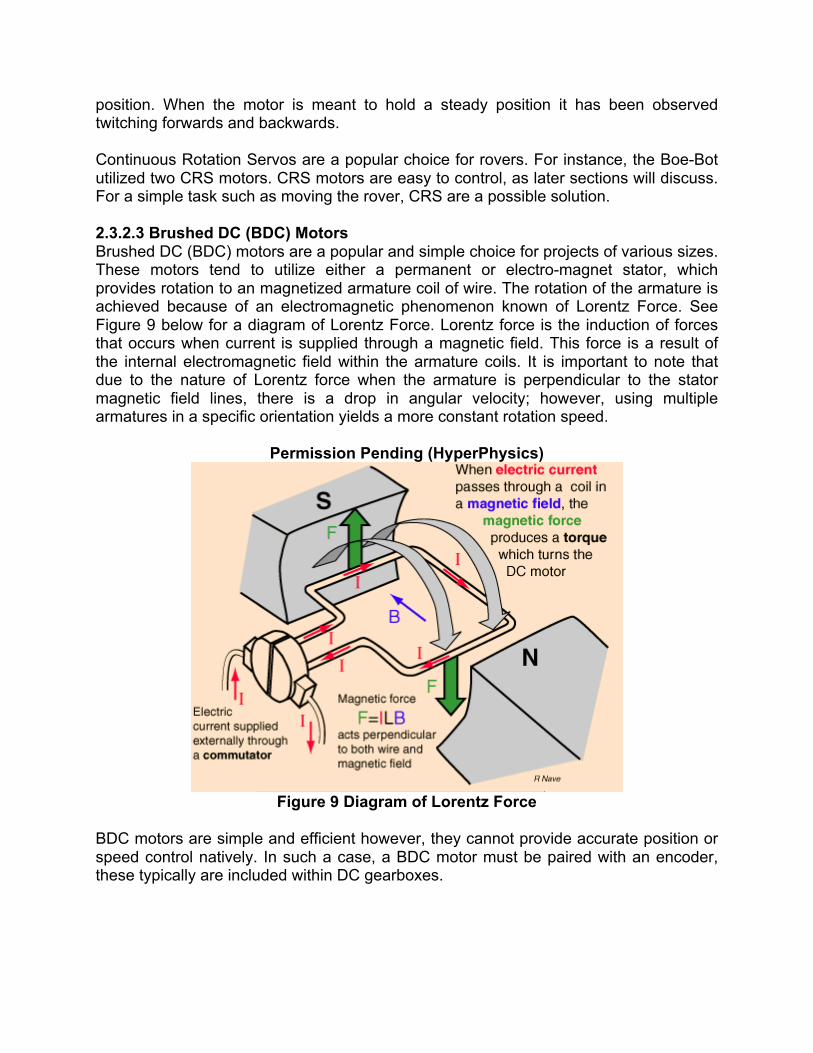
position. When the motor is meant to hold a steady position it has been observed twitching forwards and backwards. Continuous Rotation Servos are a popular choice for rovers. For instance, the Boe-Bot utilized two CRS motors. CRS motors are easy to control, as later sections will discuss. For a simple task such as moving the rover, CRS are a possible solution. 2.3.2.3 Brushed DC (BDC) Motors Brushed DC (BDC) motors are a popular and simple choice for projects of various sizes. These motors tend to utilize either a permanent or electro-magnet stator, which provides rotation to an magnetized armature coil of wire. The rotation of the armature is achieved because of an electromagnetic phenomenon known of Lorentz Force. See Figure 9 below for a diagram of Lorentz Force. Lorentz force is the induction of forces that occurs when current is supplied through a magnetic field. This force is a result of the internal electromagnetic field within the armature coils. It is important to note that due to the nature of Lorentz force when the armature is perpendicular to the stator magnetic field lines, there is a drop in angular velocity; however, using multiple armatures in a specific orientation yields a more constant rotation speed.

Permission Pending (HyperPhysics)

Figure 9 Diagram of Lorentz Force

BDC motors are simple and efficient however, they cannot provide accurate position or speed control natively. In such a case, a BDC motor must be paired with an encoder, these typically are included within DC gearboxes.

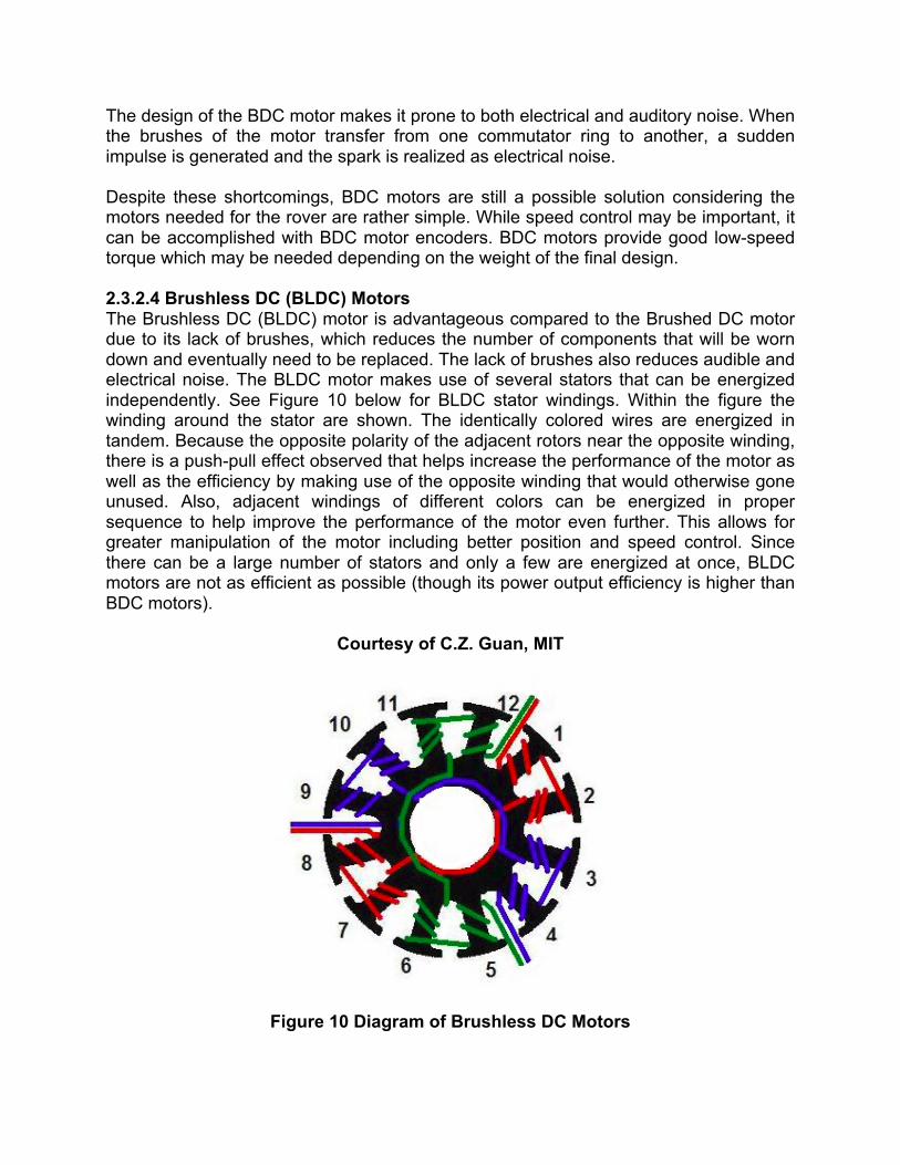
The design of the BDC motor makes it prone to both electrical and auditory noise. When the brushes of the motor transfer from one commutator ring to another, a sudden impulse is generated and the spark is realized as electrical noise. Despite these shortcomings, BDC motors are still a possible solution considering the motors needed for the rover are rather simple. While speed control may be important, it can be accomplished with BDC motor encoders. BDC motors provide good low-speed torque which may be needed depending on the weight of the final design. 2.3.2.4 Brushless DC (BLDC) Motors The Brushless DC (BLDC) motor is advantageous compared to the Brushed DC motor due to its lack of brushes, which reduces the number of components that will be worn down and eventually need to be replaced. The lack of brushes also reduces audible and electrical noise. The BLDC motor makes use of several stators that can be energized independently. See Figure 10 below for BLDC stator windings. Within the figure the winding around the stator are shown. The identically colored wires are energized in tandem. Because the opposite polarity of the adjacent rotors near the opposite winding, there is a push-pull effect observed that helps increase the performance of the motor as well as the efficiency by making use of the opposite winding that would otherwise gone unused. Also, adjacent windings of different colors can be energized in proper sequence to help improve the performance of the motor even further. This allows for greater manipulation of the motor including better position and speed control. Since there can be a large number of stators and only a few are energized at once, BLDC motors are not as efficient as possible (though its power output efficiency is higher than BDC motors).

Courtesy of C.Z. Guan, MIT

Figure 10 Diagram of Brushless DC Motors

BLDC motors come in ‘inrunner’ and ‘outrunner’ variants. The terminology refers to the location of the stator and rotor components. The inrunner configuration has the rotor within the stators whereas the outrunner has the rotor outside the stator. The function is comparable although it has been noted that the outrunners typically produce higher torque at low speeds. When using BLDC the addition of a motor controller is essential for operation. Although the electromagnetic structure is simpler than the BDC, its electrical control is more rigid. 2.3.2.5 Stepper Motors A stepper motor is a brushless DC electric motor that divides a full rotation into a number of equal steps. The stepper motor has the ability to convert a sequences of input pulses, that are typically in the form of square wave pulses, into a precisely defined increment in the shaft position. Each pulse moves the shaft through a fixed angle. Stepper motors are ideal for applications that require precise positioning because of their ability to move in precise repeatable steps. The torque of a stepper motor is maximized at low speeds and tends to dwindle at higher speeds. We want to rotate the device at relatively low speeds so a stepper motor is a viable candidate for this task. 2.3.2.6 Motor Encoders Previous sections have made reference to motor position and speed control and how these attributes can be established with the inclusion of a motor encoder. Later sections will be dedicated to motor control, which will discuss the usage of both encoders and drivers in terms of feedback looping and position reading. Within this section, motor encoders will be analyzed in regards to specific available types. This section will also cover techniques used to maximize encoder reliability and the standard practices used when operating motor encoders. A motor encoder is a supplementary device that is used in conjunction with a motor in order to allow for designers to motion and manipulate the motion of a motor. This can be achieved in a myriad of ways; however, this section will focus exclusively on rotary encoders. Rotary encoders interpret the motion of the motor by analyzing the movement of the motor shaft. This information is relayed from the sensor and is the essential aspect of controlling the motor. Since the motor shaft is analyzed rather that the stators or rotors, rotary encoders are externally connected to the motor, housing parts of the shaft. This is beneficial as it allows a variety of encoders to be paired with a given motor and the potential malfunction of an encoder can be fixed with an easy substitution of external components. Rotary encoders can be designed as either incremental or absolute encoders. The incremental encoder focuses on relative positioning and they are mainly used with AC induction motors. Using two out-of-phase square-waves, the speed, direction and position of the motor shaft can be interpreted. An absolute encoder makes use of encoded position values to give an absolute position for the entire motor shaft. The analysis of the shaft position is based on square waves also, particularly the edge transitions. Because of this, there is a maximum error given by 0.5 bits within an absolute encoder. Both incremental and absolute encoders describe simply the technique for measuring position. Both encoders can be used as an aspect of different

rotary encoder types. There are two primarily used types of rotary encoders, an optical and a magnetic variant. 2.3.2.6.1 Optical Rotary Encoders Optical rotary encoders are the most common form of encoders and uses light exposure in order to operate. Optical rotary encoders can be realized in both the incremental and absolute encoder variants. The necessary components of an optical rotary encoder include: a source of light, an encoded disk, a light detector, and a signal processor. The light source, typically an LED, sends a steady beam of light towards a pair of photodetectors. A disk that is attached to the motor shaft interrupts this beam. This is the most vital element of optical encoders. The disk is encoded and by using a signal processor to track the position of the disk, designers can interpret the motion of the motor shaft itself. There are aspects of the optical rotary encoder that can potentially cause issues when measuring position. This is dependent on the encoded disk located in the encoder. The encoded disk is made of etched metal and uses a series of transparent and opaque bands to encode the light source. The operation of the encoder may change if the disk is altered. For instance, if more bands are added to the disk, less light will pass and this can affect the encoder resolution. However, if there are too many bands, there can be a fringing effect on the light and the signal strength of the light will be degraded. This will negatively affect the accuracy of the device. To reduce the fringing of light, an additional component can be added in-between the encoded disk and the photodetectors. This device is called a mask and sharpens the light pulses before they reach the detectors. This also allows for an adjustable resolution depending on how the mask is configured. 2.3.2.6.2 Magnetic Rotary Encoders Magnetic rotary encoders are another popular choice to control motors. These encoders use alternating magnetic poles that encompass the motor shaft along with magnetic sensors to track the motion of the motor shaft. This approach contains two separate techniques of motor control. The first technique is Hall-effect sensor approach. The other is the magnetoresistive sensor approach. Both approaches offer unique functions but also come with specific limitations. These aspects will be explored thoroughly in regards to our project needs to determine whether one of these encoders will be a suitable choice. The Hall-effect sensor is built from a circular magnet with alternating north and south poles. This ring magnet is placed on a housing wheel, which is attached to the motor shaft. Within this housing are a series of sensors, which monitor the rotation of the poles of the ring magnet. By monitoring the ring magnet, it is possible to interpret the motion of the motor shaft. Since the function is based on analyzing the rotation of arbitrary magnetic poles, the Hall effect sensor is capable of monitoring motor speed however it is not suited for measuring high precision position reading along the motor shaft. In

regards to our project, a Hall-effect sensor may not be the best choice for our Rangefinder module, which depends heavily on reading accurate positions. Magnetoresistive encoders use a tachometer-like configuration where a ring magnet with alternating poles is placed along the motor shaft. Using an array of alloy strips and additional circuitry, the rotation of the ring magnet is monitored. The description and overall function of the magnetoresistive encoder is very similar to the Hall-effect sensor, however, the magnetoresistive sensors are much more sensitive and provide a more accurate speed measurement. However, the tachometer based system offer no position measurement. Given this, and the inadequate precision of the Hall-effect sensor, it would not be a good decision to utilize magnet-based encoders within the Rangefinder module. Instead it would be best to use optical encoders. 2.3.2.6.3 Encoder Operation and Specifications Due to the importance of high precision position and speed manipulation of our project, it is imperative to maximize the operation of our motor encoders in order to achieve of project specifications. There are many noted factors that can enhance the operation of encoders. Encoders have a measured specification known as resolution. The resolution of an encoder is the position points per turn the encoder is capable of reading. This is often expressed in terms of bits. For instance, a 10-bit encoder corresponds to 210 or 1024 discrete points for each turn. The higher the resolution of the encoder the higher control of the motor and the more precise the position reading will be. For our project, an encoder with the highest resolution economically possible should be selected. An equation is given to help determine the correct resolution to select for a motor encoder. It is based on multiple design specifications. It is given by:

FREQUENCY = ( N * RESOLUTION ) / 60 where frequency is measured in Hertz, N is the speed of the motor measured in revolutions per minute, and resolution is measured in points per turn. Our project has specified our frequency, with this value, a speed for the motor can be set and, using the equation above, a suitable resolution for the motor encoder would be determined. In general, it is standard practice to select a resolution that is up to four times greater than the maximum source of error within the encoder, for example the encoded disk of the optical rotary encoder. The accuracy of the encoder must also be considered when striving for high precision measurements. The accuracy of the encoder can be thought of the relation of the theoretical shaft position versus the actual shaft position. The theoretical position is what would be read by the encoder and relayed to various other components. The actual position would be where the motor shaft is position is reality. The closer the theoretical position is the actual position, the more accurate the encoder is. Accuracy is not based on resolution. A high-resolution encoder can still be inaccurate if error

between the theoretical and actual position remains. Accuracy is dependent on the entire operation of the encoder and can be affected by minute mechanical imperfections. When using optical rotary encoders, the function of the encoded disk is the primary contributor to overall accuracy. Repeatability is an important factor that deals with an encoder replicating a shaft position. This can be potentially important if our project requires a specific position to be set on the motor repeatedly. In this case, repeatability relies on the encoder reading identical codes for the position, which would allow the motor to be moved to the same position consistently. Repeatability is not dependent on the accuracy of the encoder. It simply depends on matching coded positions. If the encoder is inaccurate, a specific position will still be correctly repeated, however the repeated position may not match the actual position the designer is intending to find. Another important aspect of encoders to review is the reliability of encoders. Reliability can be viewed as the consistent operation of the encoder system. A reliable encoder will operate successfully without undesired interruptions. Reliability can be broken into two aspects: mechanical reliability and electrical reliability. Mechanical reliability deals with physical configuration of the encoder and ensuring it is structurally sound. Different encoders have different structures. For instance, encoders may or may not have ball bearings, which are used to allow the particular components to rotate freely on the motor shaft. However, these bearings are not designed for high loads and excessive weight can lead to instability. Encoders are also vulnerable to an effect known as side loading. Side loading most often occurs when the motor is run at high rpm’s and the system is hard-mounted to the motor shaft. Bearings are capable of handling high rpm’s provided there is proper lubrication and the bearing material is of good quality. Electrical reliability deals with the powering of an encoder. Encoders require precise power input and must be shielded from auxiliary components. It is considered best practice to power an encoder with filtered and regulated power. This prevents unwanted variability. To prevent interference with other components, it is best to wire other components away from the encoder cabling. It is also recommended to shield the cables by using shielded twisted pairs. For high precision applications such as this project, it is necessary to ensure that all readings are accurate and are not influenced by external factors. After an encoder measures or manipulates the position of the motor shaft it needs to relay this information. There are many different systems used for data exchange within the encoder. These include Standard Serial Output (SSO), which is used primarily with the magnetic encoders, the Synchronous Serial Interface (SSI) which is a uniform point-to-point interface, and the BiSynchronous Serial Interface (BiSS) which is compatible with SSI and can be implemented as point-to-point or bus-to-point. BiSS is a powerful and robust protocol that allows various types of information about the encoder to be sent during the operation of the encoder without interruption.

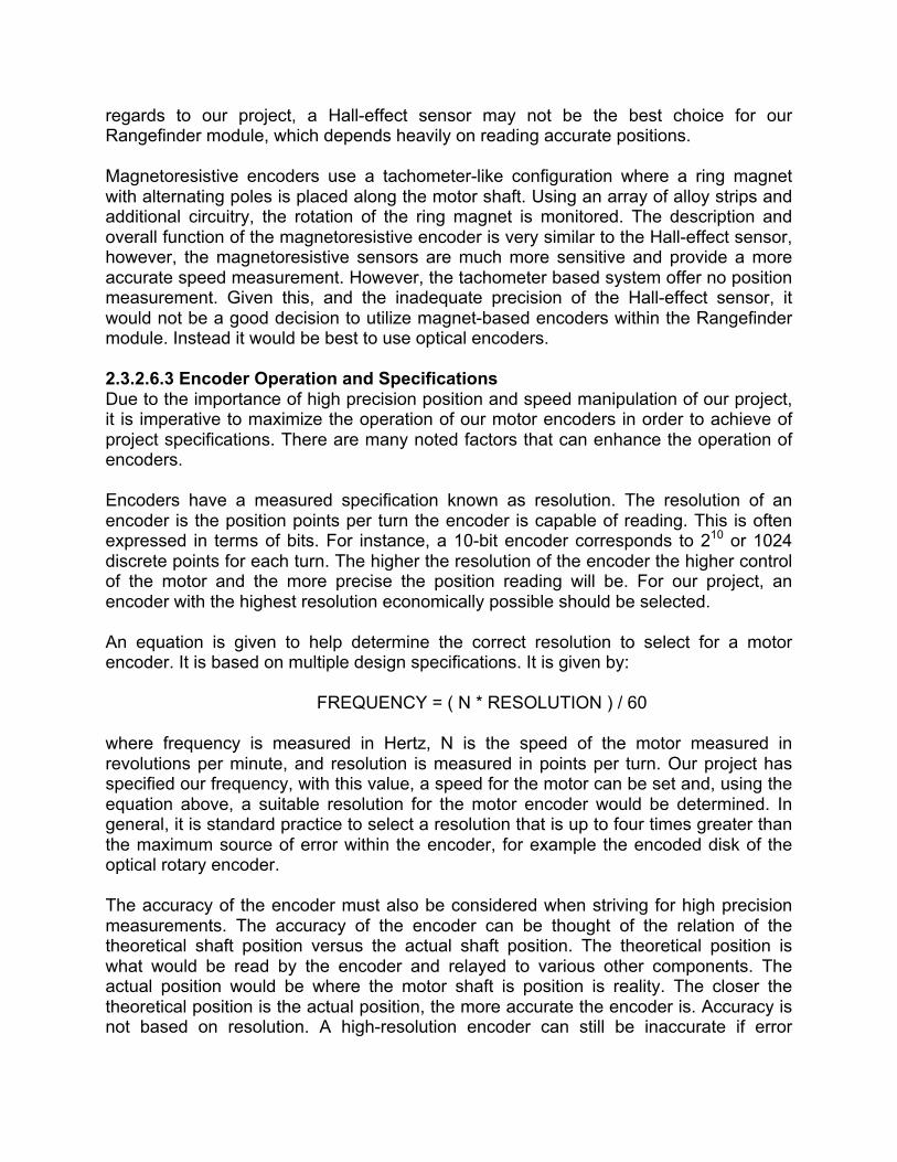
2.3.2.7 Motor Drivers Motors tend to use large amounts of power either continuously or sporadically depending on the design of the circuit. This can have a disruptive effect on additional components that may be connected to the motor. There are also issues involving power ratings of both the supply and motor that makes the safe operation of the motor incredibly important. Because of this, motor drivers are required to keep the motor from drawing dangerous amounts of current or running at too high of a voltage. The practical use of motor drivers extends beyond safety. Motor drivers are also important for assisting the motor in starting and stopping, regulating speed and torque, and controlling basic forwards and backwards rotation. There are many different types of motor drivers from the simple H-Bridge to drivers designed exclusively for each motor technology. For our project, which very likely will contain a variety of motor types, motor drivers need to be carefully explored to ensure the best components are chosen. For the motor rotating the Rangefinder module, position and speed control are vital to the success of the project. The motors that will move the rover, however, are less important and can be simple, cost-efficient.The overall budget of the project must also be taken into consideration given the varying prices of the motor drivers. 2.3.2.7.1 H-Bridges H-Bridges are a relatively simple device that aid motor control by using four switches. See Figure 11 below for detailed H-Bridge operation. These switches tend to be realized as transistors but the same function can be accomplished by replacing the transistors with relay switches. Their basic function is to allow the reversal of current, which in turn reverses the rotation of the motor.

Figure 11 H-Bridge Motor Control Design

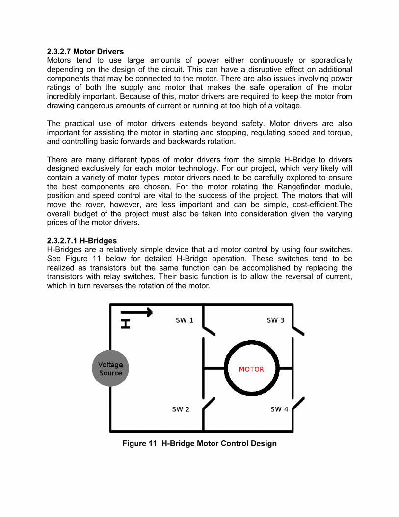
H-Bridges provide a simple solution to drive a motor forwards and backwards which explains why it is the method used to drive both standard and continuous rotation servos. See Figure 12 below for the H-Bridge operation table. It is important to pay attention to the orientation of all of the switches, as there are multiple scenarios that could potentially lead to the motor driver circuit being short-circuited. This could lead to severe damage and should be avoided whenever possible.

Figure 12 H-Bridge Motor Control Operation

H-Bridges, on the other hand, do not have any features that aid speed or position control making it a poor choice for applications requiring precision in these aspects. However, motor encoders can do the job of controlling speed and position so potentially a motor can be used with an encoder and H-Bridge and accomplish the same task of a more robust motor driver. 2.3.2.7.2 Brushed DC Motor Drivers BDC motors are incredibly simple to drive, based on project requirements. The basic task of motor drivers (speed control and direction control) can be accomplished without the need for any circuitry. In order to reduce or increase speed, one would simply decrease or increase the voltage across the BDC. In order to reverse the direction, the motor can be powered at reverse voltage. A more appropriate method of motor control that maintains its simplicity is the combination of a Pulse-Width Modulator (PWM) and transistor. The PWM controls the speed via the duty cycle of the pulses sent to the motor. The higher the duty cycle, the more power sent to the motor and the faster it goes. As discussed earlier, an H-Bridge functions well at reversing current and can be implemented in the BDC if needed. For it to be properly used a PWM is included and functions in an identical manner of the one described earlier. With the PWM controlling speed and the H-Bridge controlling direction, the combination goes both main tasks of simple motor drivers.

There is a specific IC called the L293D, which contains multiple H-Bridge transistors and PWMs. It allows a maximum of two motors to be independently controlled. In a set-up similar to the Boe-Bot, the rover can use such an IC with two motors, a trailing wheel for stability, and cheaply achieve a fully range of motion. 2.3.2.7.3 Brushless DC Motor Drivers As BLDC motors are more electrical complex, the mechanisms required to drive them are also more advanced when compared to the BDC. Most BLDC motor drivers use a built-in sensor called the Hall Effect sensor. The Hall Effect is an electromagnetic phenomenon that allows the orientation of the BLDC motor to be detected. An important aspect to the Hall Effect sensor is that it increasing the efficiency of the motor, which is needed given the inefficiency of the design which leaves many stators idle. Given that the sensor works by measuring position, it is clear that it also aids the motor in position control applications. There is another method to driving BLDC motors that does not involve an additional sensor being added. It instead relys on some of the electromagnetic properties of the BLDC motor. This property is called back-EMF. Electromagnetic forces (EMF) develop when there are electric fields, which themselves are generated by the separation of charges. Recalling the design of BLDC motors, the stators around the motor are energized in a particular sequence. As the stators are energized, a separation of charge is produced and subsequent electromagnetic fields and forces are developed. By analyzing these forces, it is possible to interpret the position and speed of the BLDC. This allows for feedback when operating the motor. 2.3.2.7.4 Stepper Motor Drivers Similar to the servo and BDC motors, the stepper motor makes use of multiple H-Bridges and PWMs. The operation is identical. There are some differences in the powering of the stepper motor, which is worth taking into consideration. The stepper motor is rated per phase and this must be accounted for when calculating power usage since there are many variants of stepper motors ranging from two to four phase. 2.3.2.8 Motor Gearboxes Motor gearboxes connect to the shaft of the motor and transfer the motion in a way that is more suitable for the project. This is accomplished by a connective system of mechanical components, primarily gears and shafts. Through the usage of gearboxes it is possible to achieve functions that may have otherwise been impossible, or underperforming. Through the usage of gears, it is possible to increase or decrease either the speed of the torque being outputted by the motor. This is possible because of gear ratios. For instance, if a gear system is set-up on the output shaft that has a ratio of 3:1, every time the output shaft rotates the first gear once, the smaller gear will rotate three times. If the wheel axle is connected to the smaller gear, the speed of the rover will have been

increased three-fold. If the ratio was reversed, the wheel axle will rotate one third of a revolution for each full revolution of the motor shaft. This is what allows for an increase in low speed torque. There are several potential issues to overcome with the usage of gearboxes. The introduction of additional components also introduce energy losses, this can be due to friction, inertia, and the heat of the gears. Another issue is known as backlash. This is the inefficient collision of gears that occur when the motor suddenly changes its direction of rotation. Slack between the gears is created and this is bad for high precision control applications. While most motors function alongside a gearbox and encoder in a highly similar fashion, stepper motors are unique due to their configuration and attributes. In previous sections, stepper motors have been explored. Among this information it is important to note the inherent precise positioning stepper motors maintain during this operation. These discrete steps that are achieved by the stepper motor have a crucial effect on how gearboxes and encoders will be applied to this motor. For instance, gearboxes are excellent at achieving high torque ranges based on gear ratios. However, due to the nature of stepper motors, low-speed torque is already at an acceptable value. The motor’s ability to maintain its position, known as holding torque, is also at an acceptable value. Additionally, the stepper motors native speed and position control have been examined which would negate the practicality of external motor control. Despite this, there are still several reasons which may justify the usage of either gearboxes with stepper motors. One such reason would involve designing a stepper motor for maintaining a specific high-speed torque. As the previous paragraph discussed, the stepper motor inherently has excellent low-speed torque, however, in order to achieve acceptable torque at high-speeds a gearbox may be needed. In regards to torque, the loading of the motor should also be taken into account. If the motor is overloaded, the motor may miss on some of its discrete steps. In this case, a gearbox may improve the motor's ability to handle large loads to due increase output torque. Another potential situation requiring a gearbox would be enhanced precision. While stepper motors come rated by their steps per revolution, the addition of a gearbox can either increase or decrease the realized shaft motion through the ratio of the gears. The efficiency of the motor is also considered when deciding whether or not to include a gearbox on the motor. Stepper motors are inherently very inefficient and can even generate large amounts of heat when driven either too fast or for too long. This can be somewhat mitigated through the usage of a gearbox. This allows the motor to run at a lower speed while maintaining its original output rotation due to the gear ratios within the gearbox. Running the motor at this lower speed reduces the chances that the motor overheats and can help maintain a slightly higher efficiency. Given all these factors, whether or not a stepper motor is paired with a gearbox is usually dependent on the application of the motor. If the project does not require a large

amount of precision or speed, the native stepper motor would likely suit the design. However, as discussed, the projects demanding a more specific torque profile, a more precise position control, heavy loading, or substantially high rotational speed will be largely benefitted through the usage of gearbox. Practically all consumer-grade motors are paired with gearboxes, as the speed of the native motor is often much higher than any applications needed by designers. For our purpose, the gearbox will need to be designed to allow for ultra-fast rotation of the Rangefinder module, in order to meet our specifications. 2.3.3 Motor Control It is important that the Base Module changes the direction of the range finder at a constant angular velocity and that the angular position is accurately measured. In order to maintain a constant angular velocity, a negative feedback loop must be created that uses the motor encoder as input and the motor driver as output. For a DC motor this means that the control system must adjust the voltage driving the motor, and then measure the angular velocity. If the angular velocity is slower than the desired speed than the voltage must be increased, and if the angular velocity is faster than the desired speed than the voltage must be decreased. The closer the actual motor speed is to the desired speed, the smaller the voltage adjustments need to be. By doing this, it is possible to control the actual angular velocity of the range finder. In order for this feedback loop to work, there are two different components that need to be addressed; The Encoder and the Motor Driver. There are many different motor drivers designed to control different types of motors. Motor drivers typically abstract the motor from the rest of the circuit by providing a convenient way of controlling the motor without having to deal with how the motor physically works. A DC motor driver for example, needs to change the voltage going through the motor in order to change the speed. This voltage does not necessarily correspond directly to the angular velocity however. For this reason it is important to use a motor encoder in order to directly measure the angular position. The purpose of a motor encoder is to provide angular position information about the rotating shaft. In general there are two types of motor encoders; Absolute and Incremental/Relative. Either type of encoder will work for the purposes of this design, however the easiest type to work with would be absolute encoders. In order for the control loop of the motor to work correctly the angular velocity in addition to absolute angular position are required. The angular velocity of the motor can be determined from the absolute position of the motor by taking the derivative. By continuously reading the absolute position of the encoder and adjusting the motor driver eventually the desired angular velocity will be reached. If the supply voltage fluctuates over time, the negative feedback loop should be able to readjust the motor driver and maintain the constant angular velocity. This is useful if the device is to be powered off of a battery because as batteries discharge the voltage tends to decrease slowly.

If a relative position encoder is chosen in the final design there is a configuration stage of the device that needs to be considered. In order to get absolute position using a relative position encoder, the device has to begin rotating from a known position. Although the device does not need absolute position for the motor control feedback loop it does need absolute position in order to get meaningful samples. The easiest way of doing this is to start at a known position and continuously measure the relative position from this point. The most common type of motor encoder used for measuring relative position is called a quadrature encoder. A quadrature encoder is a type of incremental encoder that has two signals called signal A and signal B. Signal A and B are both square waves that are 90 degrees out of phase from one another. The phase difference makes it possible to determine the direction the motor shaft is rotating. The angular position of the shaft is encoded by counting the number of times the square changes over time. If the starting position is known than the absolute angular position of the motor shaft is also known. There are a few different ways of obtaining this starting position. One way would be to place a magnet on the rotating device and use a reed switch to determine the magnets location. Every time that the magnet completes a rotation, the reed switch will trigger an event on the microcontroller signaling that a known angular position has been reached. Quadrature encoders work with any type of motor so the best kind of motor to use would be the cheapest one that can rotate at the required angular velocity. If quadrature encoders were used, then the best type of motor to use would be a DC motor because of its simplicity and price. When picking out a motor and encoder to use it is important to understand what parameters will affect the design specifications. The first parameter that is affected by the motor and encoder is the scan rate. The RPM of the motor will be the max scan rate of the device. The second parameter to think about is the number of counts per revolution that the encoder will output. The number of counts per resolution will be the max number of points per scan that can be achieved. 2.4 Range Finding Device Lidar systems are analogous to radar systems except that lidar systems use light instead of using radio waves. The device determines the distance of objects by measuring the amount of time it takes for a laser to hit an object, scatter, and bounce back to the device. At the front end of every lidar design, there will be some kind of laser and detector circuit for pulsing the laser and detecting the scattered light. For many of the design approaches, the front end will be the same, and the only difference will be the method of measuring the time of flight. In order to meet performance specifications of the scanning lidar design, the device needs to be accurate, have a few meters of range, and have a high sample rate. The higher the sample rate, the more points there can be per scan. This is important because the more points per scan the more useful the lidar data will be. These parameters will all be affected by the method used for measuring distance. The

majority of the research done was focused on determining which method of measuring distance is the best for a scanning lidar design. 2.4.1 Interface The Range Finding Module will need to interface with the Base Module using some kind of protocol. In order to choose the correct protocol to use, it is important to identify how the device should be operated. The agreed upon convention is that the range finding module should be able to accept commands in the same way that a slave device is usually expected to, however it should also be able to interrupt the Base Module when it has finished a range reading. For this purpose I2C is definitely not ideal because it does not provide a good standard way of interrupting the master when data is ready. The master device would have to continuously pull the slave device to see if data is ready. I2C is good when there are a large multitude of devices sharing the same bus, but this LIDAR system will not be taking advantage of this property. SPI would encounter all of the same problems as I2C. It is a master/slave protocol meaning that the slave can’t interrupt the master in order to initiate communication. UART is a good choice for creating a communication link between the two devices. The reason is that both modules can interrupt each other to initiate communication. In this way the Base Module can send the Range Finding Module a command to start a conversion, and the Range Finding Module can respond with the result when it is ready, or notify the Base Module if an error has occurred. Depending on the baud rate chosen for communication, there may be some limitations on scan-rate and range samples per scan. At high baud rates, the communication interface will not be a limiting factor on these specifications, however for low baud rates this could be a problem. In addition to having a UART communication port, it may also be beneficial to have a USB port so that the LIDAR can be directly plugged into a computer. This is convenient because no external hardware will be required to send data to the computer. If there was only a UART port than external hardware would be required to read the data on a PC. In addition to USB being convenient, it is also much faster than UART which will make it work much better for high scan rates. The only problem with USB is that the firmware for setting up USB is much more complex than UART. There are many drivers already written that will make setting up USB possible to integrate in a short amount of time. 2.4.2 Optics The first step to understanding how to design the laser front end circuit is to understand how to generate a laser source and then how to absorb that laser. The most common way to generate the laser pulse is to use a laser diode. When current is sent through a laser diode, it functions just like every other diode with the exception that a coherent light source is generated. This means that all of the light energy has the same

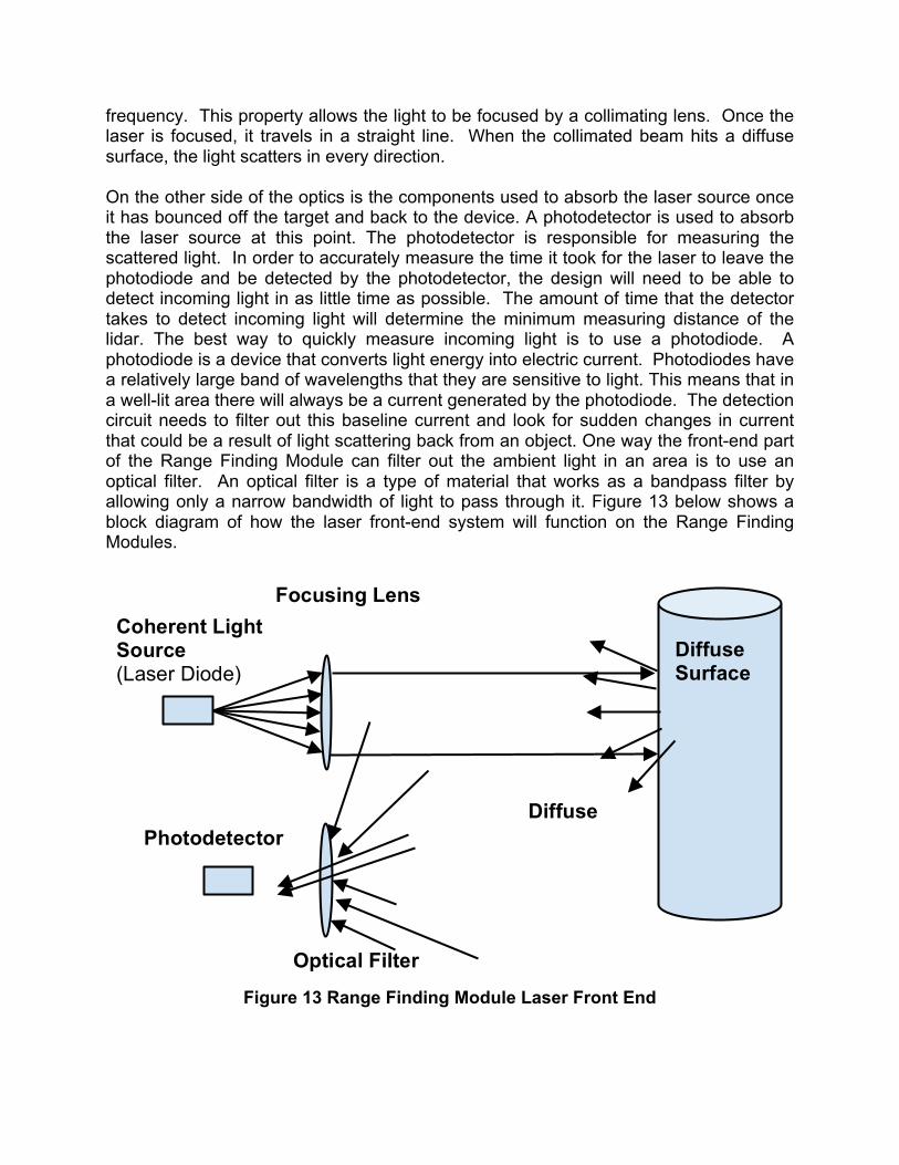
frequency. This property allows the light to be focused by a collimating lens. Once the laser is focused, it travels in a straight line. When the collimated beam hits a diffuse surface, the light scatters in every direction. On the other side of the optics is the components used to absorb the laser source once it has bounced off the target and back to the device. A photodetector is used to absorb the laser source at this point. The photodetector is responsible for measuring the scattered light. In order to accurately measure the time it took for the laser to leave the photodiode and be detected by the photodetector, the design will need to be able to detect incoming light in as little time as possible. The amount of time that the detector takes to detect incoming light will determine the minimum measuring distance of the lidar. The best way to quickly measure incoming light is to use a photodiode. A photodiode is a device that converts light energy into electric current. Photodiodes have a relatively large band of wavelengths that they are sensitive to light. This means that in a well-lit area there will always be a current generated by the photodiode. The detection circuit needs to filter out this baseline current and look for sudden changes in current that could be a result of light scattering back from an object. One way the front-end part of the Range Finding Module can filter out the ambient light in an area is to use an optical filter. An optical filter is a type of material that works as a bandpass filter by allowing only a narrow bandwidth of light to pass through it. Figure 13 below shows a block diagram of how the laser front-end system will function on the Range Finding Modules.

Figure 13 Range Finding Module Laser Front End

Diffuse Surface

Coherent Light Source (Laser Diode)

Focusing Lens

Diffuse Reflection

Optical Filter

Photodetector

Understanding the basic optical principles of the functions of the lidar are critical to understanding its specifications and constraints. For example, because the system depends on the laser light scattering in every direction, the only kind of surfaces that it can reliably detect are diffuse surfaces. The better the diffuse reflection is, the more likely the device is to detect the object. If the surface is a perfect mirror than it is impossible to detect by using a laser and photodetector. It will also be impossible to detect objects that are blackbodies at the wavelength generated by the laser diode. The device also might have trouble detecting objects when it is outdoors. The reason is that in an outdoor environment, the sun may generate a lot ambient light creating too much noise for the detection circuit to filter out. The front-end sub-module of the Range Finding Module will be responsible for generating the laser and detecting the scattered light. This responsibility imposes a few constraints on the overall system. As discussed in Section 1.4 of this document, the detection range of the device is one of these constraints. There are many factors to be considered when determining what the detection range of the Range Finding Device should be. The environment plays a major role in how far the laser will travel before it loses too much energy to be detected. In addition to the laser losing energy as it travels through the air, if the environment has a lot of ambient light at the laser’s wavelength, then the detector circuit will require more energy to scatter back to the device in order to trigger a detection. Although the two previous mentioned factors are of concern when it comes to the design of the optical section of the laser rangefinder, the main factor that will limit the range is more related to geometry. In an ideal situation, when the laser hits a target it will scatter equally in every direction. This is called a diffuse reflection. The result of this reflection is that all of the energy is dispersed evenly in every direction. This means that only a small fraction of the laser energy will make it back to the device. A BRDF, or Bidirectional Reflection Distribution Function, can be used to determine the actual amount of power making it back to the device. BRDFs are different for different objects, but for a diffuse surface, the function is relatively simple. Using a perfect diffuse surface, all of the light hitting the object is reflected evenly and symmetrically in every direction. The equations below describe how to estimate the power from the laser that is hitting the photodiode. Formula for calculating the radiance of the diffuse reflection:

𝐿 = 𝑃 / (4𝜋) L = reflected radiance, which is the power per unit solid angle P = power of the laser Formula for approximating solid angle of the detector region of the photodiode:

𝑑𝛺 = 4𝜋𝑑𝑆/𝐴 (𝒓 ∙ 𝒏) 𝑑𝛺= differential solid angle dS = differential surface area of detector A = 4𝜋𝑟!, where r is the distance of the object

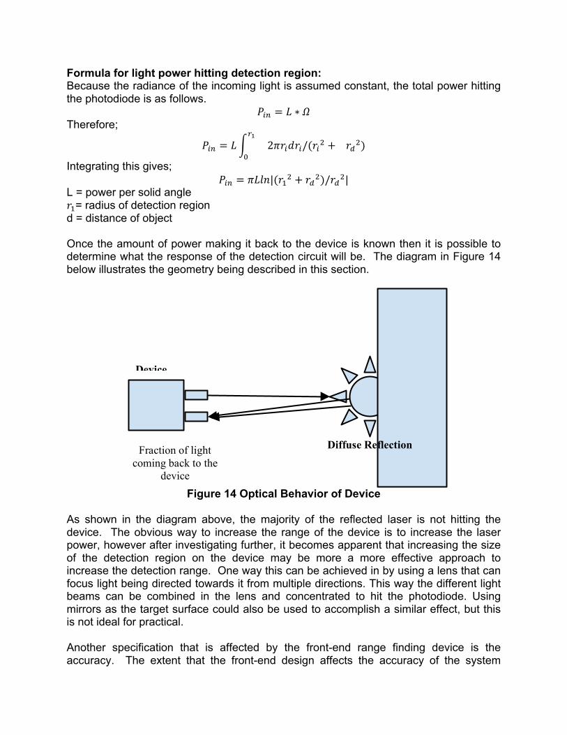
Formula for light power hitting detection region: Because the radiance of the incoming light is assumed constant, the total power hitting the photodiode is as follows.

𝑃!" = 𝐿 ∗ 𝛺 Therefore;

𝑃!" = 𝐿!!

!2𝜋𝑟!𝑑𝑟!/(𝑟!! + 𝑟!!)

Integrating this gives; 𝑃!" = 𝜋𝐿𝑙𝑛|(𝑟!! + 𝑟!!)/𝑟!!|

L = power per solid angle 𝑟!= radius of detection region d = distance of object Once the amount of power making it back to the device is known then it is possible to determine what the response of the detection circuit will be. The diagram in Figure 14 below illustrates the geometry being described in this section.

Figure 14 Optical Behavior of Device

As shown in the diagram above, the majority of the reflected laser is not hitting the device. The obvious way to increase the range of the device is to increase the laser power, however after investigating further, it becomes apparent that increasing the size of the detection region on the device may be more a more effective approach to increase the detection range. One way this can be achieved in by using a lens that can focus light being directed towards it from multiple directions. This way the different light beams can be combined in the lens and concentrated to hit the photodiode. Using mirrors as the target surface could also be used to accomplish a similar effect, but this is not ideal for practical. Another specification that is affected by the front-end range finding device is the accuracy. The extent that the front-end design affects the accuracy of the system

Diffuse

Device

Diffuse Reflection Fraction of light coming back to the

device

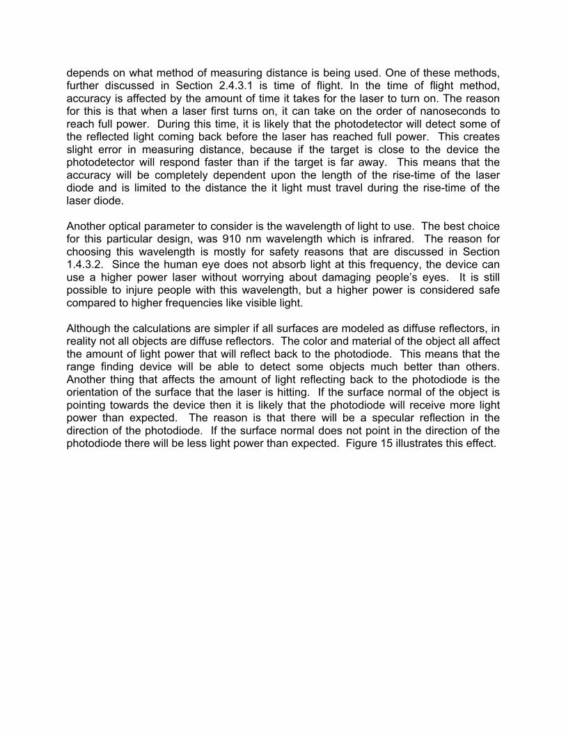
depends on what method of measuring distance is being used. One of these methods, further discussed in Section 2.4.3.1 is time of flight. In the time of flight method, accuracy is affected by the amount of time it takes for the laser to turn on. The reason for this is that when a laser first turns on, it can take on the order of nanoseconds to reach full power. During this time, it is likely that the photodetector will detect some of the reflected light coming back before the laser has reached full power. This creates slight error in measuring distance, because if the target is close to the device the photodetector will respond faster than if the target is far away. This means that the accuracy will be completely dependent upon the length of the rise-time of the laser diode and is limited to the distance the it light must travel during the rise-time of the laser diode. Another optical parameter to consider is the wavelength of light to use. The best choice for this particular design, was 910 nm wavelength which is infrared. The reason for choosing this wavelength is mostly for safety reasons that are discussed in Section 1.4.3.2. Since the human eye does not absorb light at this frequency, the device can use a higher power laser without worrying about damaging people’s eyes. It is still possible to injure people with this wavelength, but a higher power is considered safe compared to higher frequencies like visible light. Although the calculations are simpler if all surfaces are modeled as diffuse reflectors, in reality not all objects are diffuse reflectors. The color and material of the object all affect the amount of light power that will reflect back to the photodiode. This means that the range finding device will be able to detect some objects much better than others. Another thing that affects the amount of light reflecting back to the photodiode is the orientation of the surface that the laser is hitting. If the surface normal of the object is pointing towards the device then it is likely that the photodiode will receive more light power than expected. The reason is that there will be a specular reflection in the direction of the photodiode. If the surface normal does not point in the direction of the photodiode there will be less light power than expected. Figure 15 illustrates this effect.

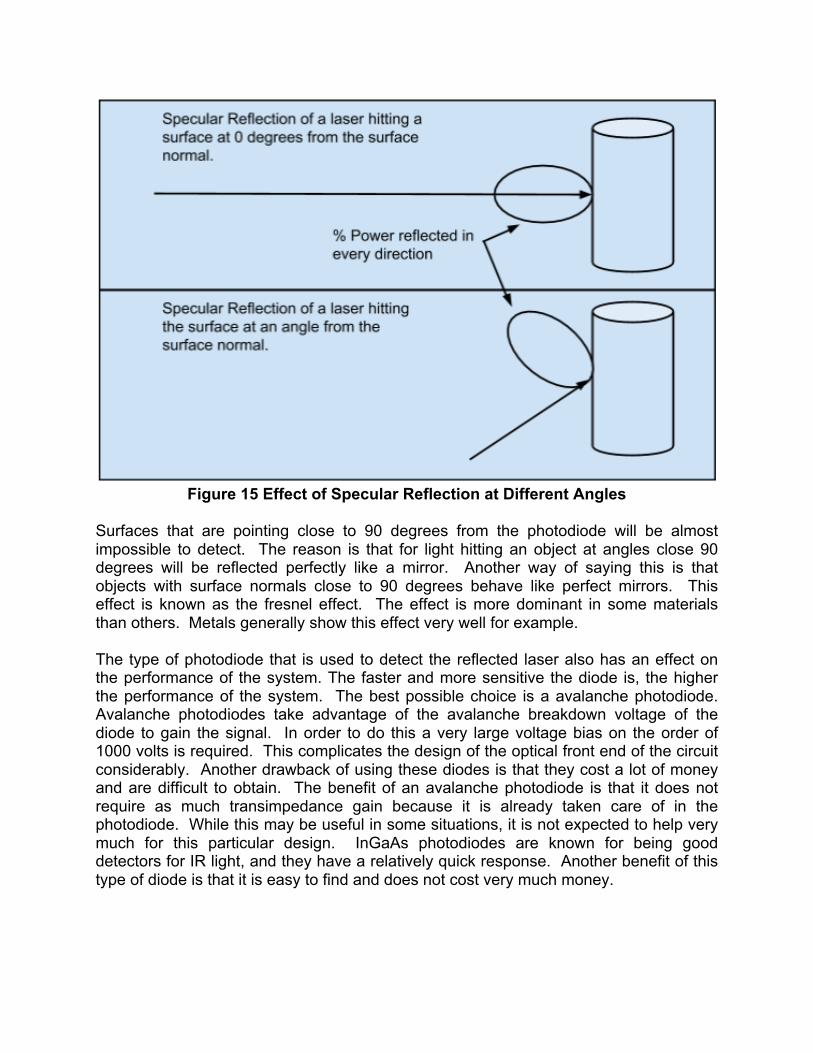
Figure 15 Effect of Specular Reflection at Different Angles

Surfaces that are pointing close to 90 degrees from the photodiode will be almost impossible to detect. The reason is that for light hitting an object at angles close 90 degrees will be reflected perfectly like a mirror. Another way of saying this is that objects with surface normals close to 90 degrees behave like perfect mirrors. This effect is known as the fresnel effect. The effect is more dominant in some materials than others. Metals generally show this effect very well for example. The type of photodiode that is used to detect the reflected laser also has an effect on the performance of the system. The faster and more sensitive the diode is, the higher the performance of the system. The best possible choice is a avalanche photodiode. Avalanche photodiodes take advantage of the avalanche breakdown voltage of the diode to gain the signal. In order to do this a very large voltage bias on the order of 1000 volts is required. This complicates the design of the optical front end of the circuit considerably. Another drawback of using these diodes is that they cost a lot of money and are difficult to obtain. The benefit of an avalanche photodiode is that it does not require as much transimpedance gain because it is already taken care of in the photodiode. While this may be useful in some situations, it is not expected to help very much for this particular design. InGaAs photodiodes are known for being good detectors for IR light, and they have a relatively quick response. Another benefit of this type of diode is that it is easy to find and does not cost very much money.

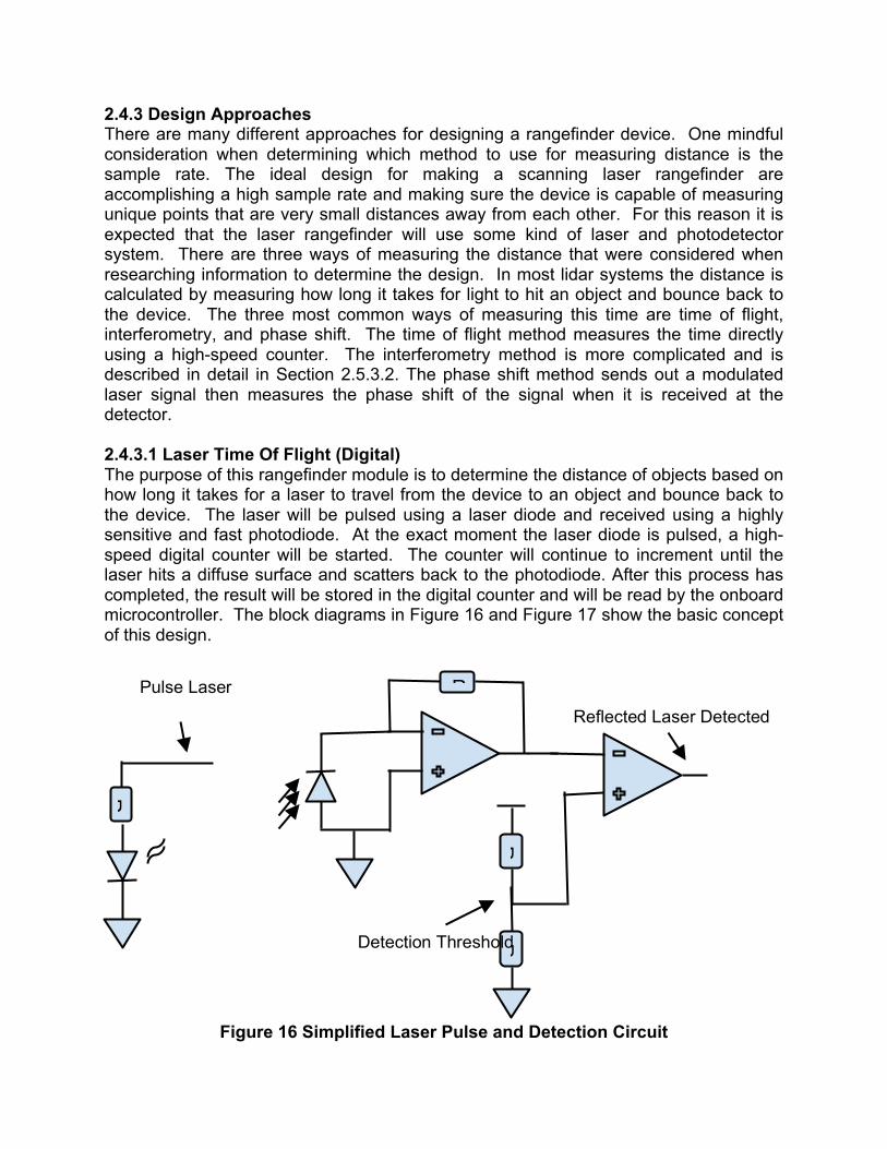
2.4.3 Design Approaches There are many different approaches for designing a rangefinder device. One mindful consideration when determining which method to use for measuring distance is the sample rate. The ideal design for making a scanning laser rangefinder are accomplishing a high sample rate and making sure the device is capable of measuring unique points that are very small distances away from each other. For this reason it is expected that the laser rangefinder will use some kind of laser and photodetector system. There are three ways of measuring the distance that were considered when researching information to determine the design. In most lidar systems the distance is calculated by measuring how long it takes for light to hit an object and bounce back to the device. The three most common ways of measuring this time are time of flight, interferometry, and phase shift. The time of flight method measures the time directly using a high-speed counter. The interferometry method is more complicated and is described in detail in Section 2.5.3.2. The phase shift method sends out a modulated laser signal then measures the phase shift of the signal when it is received at the detector. 2.4.3.1 Laser Time Of Flight (Digital) The purpose of this rangefinder module is to determine the distance of objects based on how long it takes for a laser to travel from the device to an object and bounce back to the device. The laser will be pulsed using a laser diode and received using a highly sensitive and fast photodiode. At the exact moment the laser diode is pulsed, a high-speed digital counter will be started. The counter will continue to increment until the laser hits a diffuse surface and scatters back to the photodiode. After this process has completed, the result will be stored in the digital counter and will be read by the onboard microcontroller. The block diagrams in Figure 16 and Figure 17 show the basic concept of this design.

Figure 16 Simplified Laser Pulse and Detection Circuit

R

R

R

Detection Threshold

Reflected Laser Detected

R

Pulse Laser

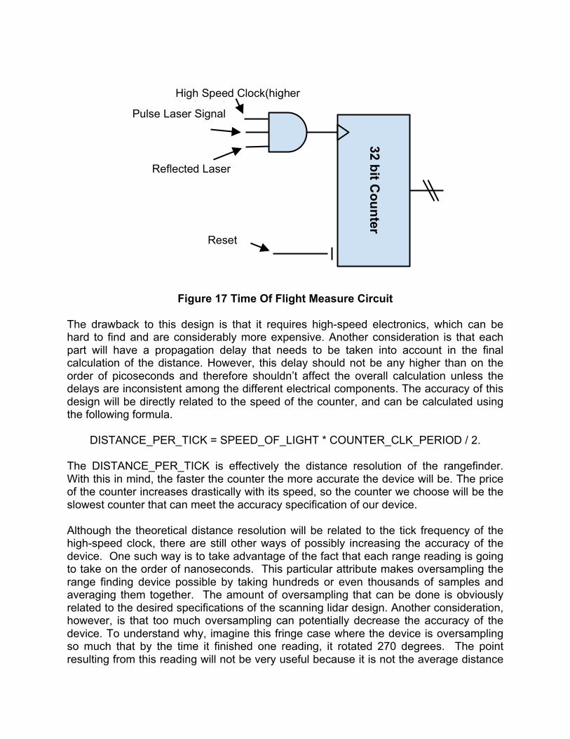
Figure 17 Time Of Flight Measure Circuit

The drawback to this design is that it requires high-speed electronics, which can be hard to find and are considerably more expensive. Another consideration is that each part will have a propagation delay that needs to be taken into account in the final calculation of the distance. However, this delay should not be any higher than on the order of picoseconds and therefore shouldn’t affect the overall calculation unless the delays are inconsistent among the different electrical components. The accuracy of this design will be directly related to the speed of the counter, and can be calculated using the following formula.

DISTANCE_PER_TICK = SPEED_OF_LIGHT * COUNTER_CLK_PERIOD / 2. The DISTANCE_PER_TICK is effectively the distance resolution of the rangefinder. With this in mind, the faster the counter the more accurate the device will be. The price of the counter increases drastically with its speed, so the counter we choose will be the slowest counter that can meet the accuracy specification of our device. Although the theoretical distance resolution will be related to the tick frequency of the high-speed clock, there are still other ways of possibly increasing the accuracy of the device. One such way is to take advantage of the fact that each range reading is going to take on the order of nanoseconds. This particular attribute makes oversampling the range finding device possible by taking hundreds or even thousands of samples and averaging them together. The amount of oversampling that can be done is obviously related to the desired specifications of the scanning lidar design. Another consideration, however, is that too much oversampling can potentially decrease the accuracy of the device. To understand why, imagine this fringe case where the device is oversampling so much that by the time it finished one reading, it rotated 270 degrees. The point resulting from this reading will not be very useful because it is not the average distance

Counter V

alue

R

ST

32 bit Counter

High Speed Clock(higher the better)

Pulse Laser Signal

Reflected Laser Detection Signal

Reset Counter

of a particular point in space, but rather an average distance of every point surrounding the device. The same problem occurs if the rangefinder moves 1.0 degrees between the start and finish of a reading. The amount of time it takes to complete a single reading also has an effect on the overall accuracy of the system. A balance exists between the amount of oversampling and the amount of time it takes to get a reading that will generate the most accurate reading. To understand this balance there is a property of lasers that needs to be mentioned. Many laser diodes available do not travel in a perfectly straight line. Instead, they spread out in a cone shape. It is this cone that defines how long to oversample each point. To figure out this time there are two important events in the distance reading; the time to start oversampling, and the time to stop oversampling. At the start time (t = 0), oversampling begins. At this time the laser cone will be at a particular place in space. For the most accurate reading, it is recommended to continue oversampling until 50% of the cone’s solid angle is outside of the starting cone. After this moment in time, the majority of the laser power is hitting a different location in space and so the range finding device is measuring a different location. Another important consideration of this design is the accuracy of the high-speed clock. A voltage-controlled clock is a good choice for generating a high frequency clock but it may need additional circuitry in order to be accurate enough for this design. The best way to generate an accurate clock will be to use a Phase Locked Loop (PLL). In addition to an accurate high frequency clock, a binary counter that can be incremented at the same speed as the high frequency clock will also be required. The fastest binary counters available for purchase are about 2 Ghz. Using this method limits the accuracy of the range finding device to about 7.5 cm. One way of doubling the accuracy is to use two binary counters. One counter can increment on the rising edge of the clock and the other can increment on the falling edge of the clock. The block diagram below shows this design in detail. Once the laser is pulsed and detected, the round trip time will be the sum of the values stored in both counters. The two counters could be read in by the microcontroller, or they could be latched and added in hardware then read by the microcontroller. Using this method, the accuracy of the device will be about 3.75 cm (+/- 1.875 cm). This is not taking into account oversampling which will further increase the accuracy of the device. The advantage of this design is that it is easy to understand, and the device specifications are well defined. For example, the sample rate and accuracy can be calculated using a simple formula. The disadvantage of this design is that many of the parts required will be hard to find, and could also potentially cost a lot of money depending on the level of functionality we strive to achieve. Not only could this design be costly, but implementing this design could also be very difficult because there are many considerations that come into effect when dealing with clock signals that are in the GHz range. At these frequencies PCB trace widths, trace lengths, substrate thickness, and substrate material also must be considered when laying out the circuit board. Once the PCB is manufactured, debugging the board will be very difficult because any kind of device capable of measuring a 2 Ghz signals will cost hundreds of

thousands of dollars. The test procedures for this board would be to pulse the laser then check what the counter values are, and determine if the values correspond to the distance being measured. If the device isn’t working, it will be difficult to determine what particular part of the circuit is not behaving correctly. The fundamental problem that requires the most consideration for the design of the laser rangefinder is how accurately the device can measure time. Devices that do this are called time to digital converters. There are many integrated circuits that perform this exact task very well. One particular part found on Digikey is capable of measuring time with a resolution of 55 ps, which will be more than enough accuracy for the purpose of building a lidar. With a 55 ps counter resolution, the accuracy of the device will theoretically be (+/-8 mm). It is expected that when the design is actually implemented, the accuracy will not be this good because of jitter of discrete circuit elements that have not been considered during initial research. Once the first prototype is built the actual accuracy of the device will be calculated to make sure the device meets the design specification. Another consideration that could affect the design is that the Time to Digital converter has a propagation delay of 10ns, so the minimum time that can be measured is 10 ns. This would mean that the minimum distance that can be measured is 1.5m. This problem can be solved by starting the counter 10ns before the laser is pulsed allowing the counter to start at the exact moment the laser is pulsed and eliminating the minimum distance specification. The benefit of using a Time to Digital converter is that it allows the design to avoid using high-speed electronics and running traces on the PCB that can handle GHz transmission. This not only simplifies the design, but also reduces the price drastically. Using this method, the total accuracy of the device will not be limited just to the resolution of the clock, but also to the amount of time it takes for the laser diode to reach full power. This time is known as the rise time. A typical laser diode will have a rise time of about 1.0ns. This will make the accuracy of the device be (+/-) 0.3 m. There are many diodes available that have higher performance than this, but they will cost more money. The reason the rise time affects the accuracy of the device is best shown in a diagram. This is illustrated below in Figure 18.

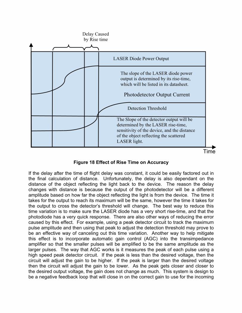
Figure 18 Effect of Rise Time on Accuracy

If the delay after the time of flight delay was constant, it could be easily factored out in the final calculation of distance. Unfortunately, the delay is also dependant on the distance of the object reflecting the light back to the device. The reason the delay changes with distance is because the output of the photodetector will be a different amplitude based on how far the object reflecting the light is from the device. The time it takes for the output to reach its maximum will be the same, however the time it takes for the output to cross the detector’s threshold will change. The best way to reduce this time variation is to make sure the LASER diode has a very short rise-time, and that the photodiode has a very quick response. There are also other ways of reducing the error caused by this effect. For example, using a peak detector circuit to track the maximum pulse amplitude and then using that peak to adjust the detection threshold may prove to be an effective way of canceling out this time variation. Another way to help mitigate this effect is to incorporate automatic gain control (AGC) into the transimpedance amplifier so that the smaller pulses will be amplified to be the same amplitude as the larger pulses. The way that AGC works is it measures the peak of each pulse using a high speed peak detector circuit. If the peak is less than the desired voltage, then the circuit will adjust the gain to be higher. If the peak is larger than the desired voltage then the circuit will adjust the gain to be lower. As the peak gets closer and closer to the desired output voltage, the gain does not change as much. This system is design to be a negative feedback loop that will close in on the correct gain to use for the incoming

LASER Diode Power Output

Time

Photodetector Output Current

Detection Threshold

Time Of Flight

The slope of the LASER diode power output is determined by its rise-time, which will be listed in its datasheet.

Delay Caused by Rise time of LASER

The Slope of the detector output will be determined by the LASER rise-time, sensitivity of the device, and the distance of the object reflecting the scattered LASER light.

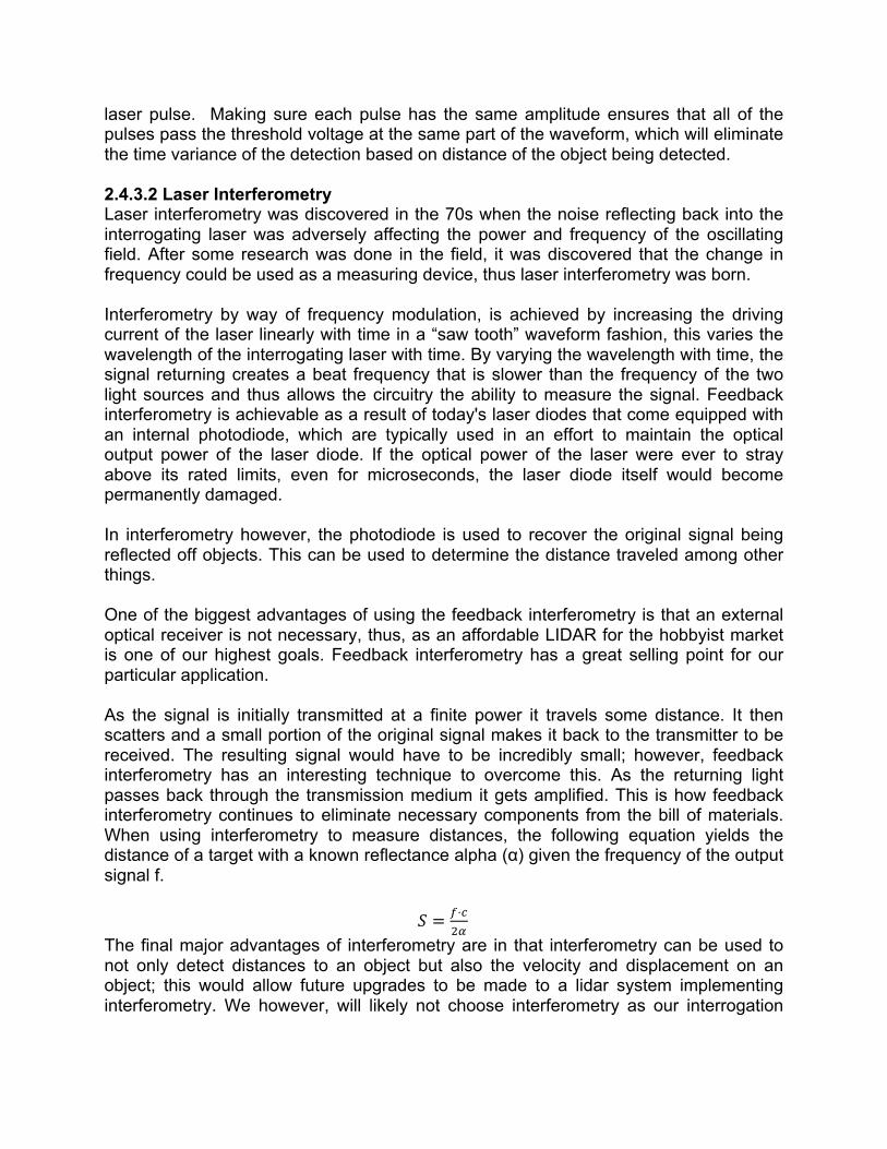
laser pulse. Making sure each pulse has the same amplitude ensures that all of the pulses pass the threshold voltage at the same part of the waveform, which will eliminate the time variance of the detection based on distance of the object being detected. 2.4.3.2 Laser Interferometry Laser interferometry was discovered in the 70s when the noise reflecting back into the interrogating laser was adversely affecting the power and frequency of the oscillating field. After some research was done in the field, it was discovered that the change in frequency could be used as a measuring device, thus laser interferometry was born. Interferometry by way of frequency modulation, is achieved by increasing the driving current of the laser linearly with time in a “saw tooth” waveform fashion, this varies the wavelength of the interrogating laser with time. By varying the wavelength with time, the signal returning creates a beat frequency that is slower than the frequency of the two light sources and thus allows the circuitry the ability to measure the signal. Feedback interferometry is achievable as a result of today's laser diodes that come equipped with an internal photodiode, which are typically used in an effort to maintain the optical output power of the laser diode. If the optical power of the laser were ever to stray above its rated limits, even for microseconds, the laser diode itself would become permanently damaged. In interferometry however, the photodiode is used to recover the original signal being reflected off objects. This can be used to determine the distance traveled among other things. One of the biggest advantages of using the feedback interferometry is that an external optical receiver is not necessary, thus, as an affordable LIDAR for the hobbyist market is one of our highest goals. Feedback interferometry has a great selling point for our particular application. As the signal is initially transmitted at a finite power it travels some distance. It then scatters and a small portion of the original signal makes it back to the transmitter to be received. The resulting signal would have to be incredibly small; however, feedback interferometry has an interesting technique to overcome this. As the returning light passes back through the transmission medium it gets amplified. This is how feedback interferometry continues to eliminate necessary components from the bill of materials. When using interferometry to measure distances, the following equation yields the distance of a target with a known reflectance alpha (α) given the frequency of the output signal f.

𝑆 = !⋅!!!

The final major advantages of interferometry are in that interferometry can be used to not only detect distances to an object but also the velocity and displacement on an object; this would allow future upgrades to be made to a lidar system implementing interferometry. We however, will likely not choose interferometry as our interrogation

method as it requires very complex math to be performed in order to be implemented effectively. 2.4.3.3 Laser Phase Shift Laser phase shift is another useful technique that can measure distance. This system essentially measures the phase difference of a transmitted and received modulated power waveform. Using the phase difference, it is possible to calculate the time of flight of the signal. With time of flight calculated, it is easy to derive the distance from the transmitter to the object. The phase shift equation is given by:

PHASE SHIFT = 2 * PI * MODULATION FREQUENCY * TIME OF FLIGHT Since the modulation frequency is set by design, and the phase shift is being observed, it is possible to solve for the time of flight of the signal. However, it is also possible to calculate the distance with the phase shift, the distance equation is as given.

DISTANCE = ½ * SPEED OF LIGHT * PHASE SHIFT / (2 * PI) * MODULATION FREQUENCY

It is important to note that the preciseness of the distance measurement depends highly on the modulation frequency. Most of the time, it is possible to modulate the laser by directly altering the drive current of the device. The higher the modulation frequency the higher the resolution of the phase shift measurement and the more precise the distance measurement. However, high-precision power modulation can potentially be too expensive for the goals of our project. Received signal power is another factor to address. Depending on the area of the lenses of the photodiodes and the transmission of the laser, the power of the reflected signal can be maximized which could reduce error when calculating distance and remove the possibility of electrical or laser noise disrupting the data points being collected. If phase shift is used, additional components may be needed. In order to properly modulate the optical power being sent out, a device known as a electro-optic modulator (EOM) must be used. EOMs can control the power, phase, or polarization of connected lasers. For our application, the power is what needs to be modulated, so designs pertaining to amplitude modulation are being explored to find a suitable solution. The amplitude modulator is built from a combination of polarizers, which encompass a device called a Pockel cell. The Pockel cell is a longitudinal device that the laser travels through. The device also has an internal electric field and two outer electrodes, which allows for the amplitude of the laser to be modulated by an electrical voltage. Due to the high costs of Pockel cells, it may be necessary to investigate different methods of power modulation. One alternative is the power modulation possible by using a mode-locked laser. Mode locking is a technique that can be applied to a laser

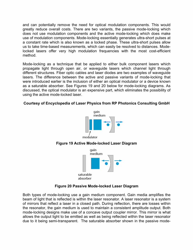
and can potentially remove the need for optical modulation components. This would greatly reduce overall costs. There are two variants, the passive mode-locking which does not use modulation components and the active mode-locking which does make use of modulation components. Mode-locking essentially generates ultra-short pulses at a constant rate which is also known as a locked phase. These ultra-short pulses allow us to take time-based measurements, which can easily be resolved to distances. Mode-locked lasers offer very high modulation frequencies with the most cost-efficient method. Mode-locking as a technique that be applied to either bulk component lasers which propagate light through open air, or waveguide lasers which channel light through different structures. Fiber optic cables and laser diodes are two examples of waveguide lasers. The difference between the active and passive variants of mode-locking that were introduced earlier is the inclusion of either an optical modulator or a device known as a saturable absorber. See Figures 19 and 20 below for mode-locking diagrams. As discussed, the optical modulator is an expensive part, which eliminates the possibility of using the active mode-locked laser. Courtesy of Encyclopedia of Laser Physics from RP Photonics Consulting GmbH

Figure 19 Active Mode-locked Laser Diagram

Figure 20 Passive Mode-locked Laser Diagram

Both types of mode-locking use a gain medium component. Gain media amplifies the beam of light that is reflected is within the laser resonator. A laser resonator is a system of mirrors that reflect a laser in a closed path. During reflection, there are losses within the resonator, the gain medium is used to maintain a consistent amplitude output. Both mode-locking designs make use of a concave output coupler mirror. This mirror is what allows the output light to be emitted as well as being reflected within the laser resonator due to it being semi-transparent. The saturable absorber shown in the passive mode-

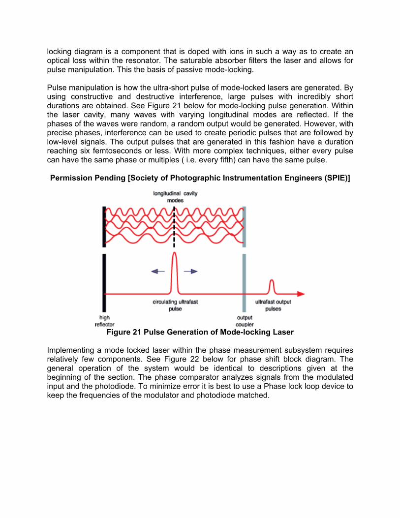
locking diagram is a component that is doped with ions in such a way as to create an optical loss within the resonator. The saturable absorber filters the laser and allows for pulse manipulation. This the basis of passive mode-locking. Pulse manipulation is how the ultra-short pulse of mode-locked lasers are generated. By using constructive and destructive interference, large pulses with incredibly short durations are obtained. See Figure 21 below for mode-locking pulse generation. Within the laser cavity, many waves with varying longitudinal modes are reflected. If the phases of the waves were random, a random output would be generated. However, with precise phases, interference can be used to create periodic pulses that are followed by low-level signals. The output pulses that are generated in this fashion have a duration reaching six femtoseconds or less. With more complex techniques, either every pulse can have the same phase or multiples ( i.e. every fifth) can have the same pulse. Permission Pending [Society of Photographic Instrumentation Engineers (SPIE)]

Figure 21 Pulse Generation of Mode-locking Laser

Implementing a mode locked laser within the phase measurement subsystem requires relatively few components. See Figure 22 below for phase shift block diagram. The general operation of the system would be identical to descriptions given at the beginning of the section. The phase comparator analyzes signals from the modulated input and the photodiode. To minimize error it is best to use a Phase lock loop device to keep the frequencies of the modulator and photodiode matched.

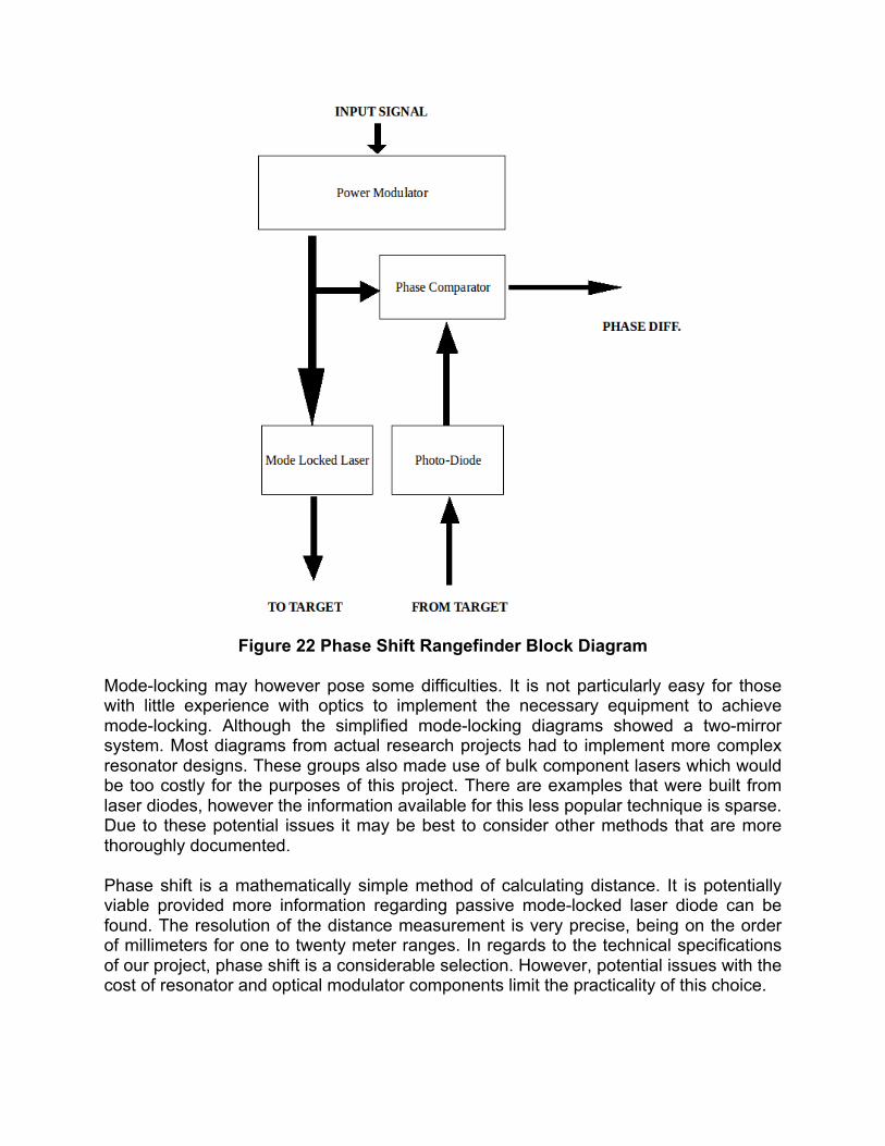
Figure 22 Phase Shift Rangefinder Block Diagram Mode-locking may however pose some difficulties. It is not particularly easy for those with little experience with optics to implement the necessary equipment to achieve mode-locking. Although the simplified mode-locking diagrams showed a two-mirror system. Most diagrams from actual research projects had to implement more complex resonator designs. These groups also made use of bulk component lasers which would be too costly for the purposes of this project. There are examples that were built from laser diodes, however the information available for this less popular technique is sparse. Due to these potential issues it may be best to consider other methods that are more thoroughly documented. Phase shift is a mathematically simple method of calculating distance. It is potentially viable provided more information regarding passive mode-locked laser diode can be found. The resolution of the distance measurement is very precise, being on the order of millimeters for one to twenty meter ranges. In regards to the technical specifications of our project, phase shift is a considerable selection. However, potential issues with the cost of resonator and optical modulator components limit the practicality of this choice.

2.4.3.4 Pulse Amplitude Another possible way of determining distance of objects is to send a LASER pulse out and then measure the amplitude of the returning signal. The closer an object is the larger the pulse and the farther the object the smaller the pulse is. There are a few obvious problems with this method. One problem is that the pulse amplitude is different for different objects and different orientations of surfaces. This means that the device will only be able to measure certain types of objects accurately. The types of objects that it can measure accurately will depend on what the device has been calibrated to detect. This makes the device considerably less useful for mapping areas however it may still be useful in some environments. The only real benefit to this method of measuring distance is that it is considerably easier to implement than some of the other methods that need to compute the time of flight of light. This means it does not require any of the fast circuitry and responsive detection elements. This simplification of the problem will make building the device much cheaper. This decision should not be considered unless none of the other design approaches work. The drawbacks that come with this design are certainly not ideal however the functionality could be considered an acceptable last resort solution. 2.5 Power Management Providing the system with power is tantamount to the success of our project. There are countless methods to provide power, however the design of our project narrows our possibilities. Given the mobile nature of our project, a battery system will be used, to increase usability, it was decided that a secondary (rechargeable) battery technology would be used. 2.5.1. Battery Technologies There are many other factors that must be considered when selecting a battery. These include: ● Power density - determines the battery’s weight for a fixed amount of stored

power ● Charge capacity - determines how long a battery can run at a fixed power rate ● Charge capability - determines how much current can be charged or discharged

at once ● Nominal cell voltage - determines power aspects of the battery given steady

current There are many different secondary battery chemistries that have been introduced spanning several decades. From the early Nickel-Cadmium cells of the 50’s to the cutting edge Lithium Polymer developed within the last fifteen years, each variant has its benefits and pitfalls. In order to select the best candidate each of the previously stated factors will be analyzed for several different chemistries. It is possible to concisely compare the attributes of the different battery chemistries by using a chart with the desired features listed. See Figure 23 below for battery technology comparisons. In regards to our project, several factors are of utmost importance.

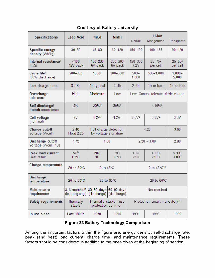
Courtesy of Battery University

Figure 23 Battery Technology Comparison

Among the important factors within the figure are: energy density, self-discharge rate, peak (and best) load current, charge time, and maintenance requirements. These factors should be considered in addition to the ones given at the beginning of section.

Since our project is mobile, the overall weight of the rover should be precisely monitored. A rover that is too heavy require more power to drive the rover motors, which will drive up the overall power consumption of the project. Although many factors will contribute to the final weight of the rover, one place where weight can be cut is in the battery. This can be achieved by selected a battery with a large gravimetric energy density, for every kilogram of weight added by the battery, there should be substantially more power added in the form of Watt-hours. It is important to distinguish between gravimetric energy density and energy density as the former measures energy per unit mass and the latter measures energy per unit volume. The higher the gravimetric energy density, the more lightweight the battery can be. Therefore, batteries with low gravimetric energy densities, such as Lead-Acid should be avoided. The other chemistries listed each offer an adequate gravimetric energy density. Another factor to consider is the self-discharge rate of the battery. Even when a battery is not connected to a circuit, it drains due to the internal resistance of the battery. The self-discharge rate will dictate how long it takes our dormant battery to lose charge. This will also play a role in determining the overall battery life of our project. It is best to select a battery chemistry that minimizes self-discharge in order to prolong the lifespan of the battery between recharging periods. While Nickel-Metal Hydride is well suited for our projected in many areas, it has a relatively high self-discharge rate. It should be noted that the self-discharge is given over the period of one month, considering this Nickel-Metal Hydride may still be a practical choice. Load current refers to the maximum amount of drawable current each battery supplies. It is measured in terms of charge capability, a percentage of charge capacity. For instance, if a battery is rated at a charge capacity of 50mAh this means the battery can power a circuit drawing 5 mA for 10 hours. However, batteries have real-word limitations for how much current can be drawn at once. To give a more detailed description of the battery, the charge capability measurement is given. Charge capability gives what portion of the charge capacity can be drawn at once. If charge capacity measures how much energy is stored, charge capability measures how long it takes to deliver that energy. Charge capability is often referred to as C-rate. If the same battery was rated at a charge capability of 0.5 C it would mean that the battery can deliver 25 mA for 2 hours. C rates give the discharge rate, 1C is referred to as the one-hour discharge, 0.5 corresponds to the two-hour discharge, 0.1 the ten-hour discharge. Given this, the higher the battery’s load current the more power can be delivered. This feature is also tied with charge time, as the battery is capable of being supplied more current at once and recharges at a faster rate. From the figure, it is shown that the lithium-based chemistries provide the best charge and discharge rates. The capacity of the battery can be improved by connected multiple batteries in parallel, however this is not considered a safe process for certain battery chemistries such as lithium-based batteries. Nominal cell voltage is important as it correlates to power, the voltage can be improved by connecting batteries in series, however, and it is not recommended for all battery

chemistries. The lithium-based batteries have the highest nominal cell voltage at nearly triple the alternative chemistries. The final factor covered in this section is maintenance requirements. Since lithium-based batteries do not have any required maintenance it is the most preferred. However, lithium-based batteries can be potentially dangerous if not operated correctly and come with a full set of safety procedures to ensure a long and safe battery life. Several safeties for lithium-based batteries procedures will be discussed in later sections. Looking at the figure, and noting the most crucial specifications described earlier, it was found that either lithium-ion (Li-Ion) or lithium-polymer (Li-Po) batteries were the superior choice. They combine excellent gravimetric energy density with great load current and recharge rates. They also have a high cell voltage and low self-discharge rate. It was also found that the cost of the lithium-based batteries was within similar ranges for the alternative chemistries. The future sections will discuss battery solutions exclusively for these two technologies. 2.5.1.1 Lithium-Ion Lithium Ion (Li-Ion) is a powerful secondary battery technology that is widely popular within the industry. While it has excellent power density, power capacity, and charge capability, it requires extreme care when charging or discharging. Separate components must be included to ensure the safe operation of both Li-Ion and Li-Po batteries. Both Li-Ion and Li-Po have a high nominal voltage at 3.6-3.8 V, which allows a high power capacity. Li-Ion batteries typically come in either rectangular or cylindrical packages and are rated in a large range of charge capacities. Li-Ion and Li-Po also benefit from not having the “memory effect” of the older battery chemistries. The memory effect essentially requires that the battery be as close to fully discharged as possible before recharging, otherwise the overall capacity of the battery will be degraded. The lack of a memory effect improves the simplicity of usage since users do not need to pay attention to discharge levels and can freely recharge when they want. Li-Ion has a few drawbacks. As mentioned, both of the lithium-based chemistries require a protection circuit for safe operation. It has also been noted that the Li-Ion battery suffers from age-degradation. While practically all batteries have this issue, it was noted that the Li-Ion battery begins to fail within three to five years regardless of its usage. Li-Ion is also older than Li-Po so there is additional benefits that Li-Ion would not be able to take advantage of. 2.5.1.2. Lithium-Polymer A relatively new technology with many similarities to Li-Ion. Lithium-Polymer (LiPo) has a higher gravimetric energy density than Li-Ion, which can allow for a lighter rover while maintaining its power output. Li-Po batteries also have a better form-factor. While Li-Ion batteries typically come in rectangular and cylindrical packages, Li-Po is capable of

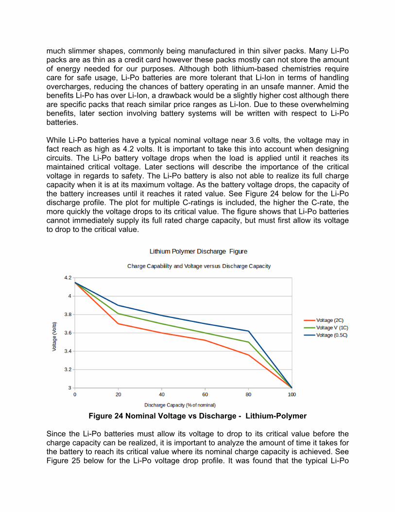
much slimmer shapes, commonly being manufactured in thin silver packs. Many Li-Po packs are as thin as a credit card however these packs mostly can not store the amount of energy needed for our purposes. Although both lithium-based chemistries require care for safe usage, Li-Po batteries are more tolerant that Li-Ion in terms of handling overcharges, reducing the chances of battery operating in an unsafe manner. Amid the benefits Li-Po has over Li-Ion, a drawback would be a slightly higher cost although there are specific packs that reach similar price ranges as Li-Ion. Due to these overwhelming benefits, later section involving battery systems will be written with respect to Li-Po batteries. While Li-Po batteries have a typical nominal voltage near 3.6 volts, the voltage may in fact reach as high as 4.2 volts. It is important to take this into account when designing circuits. The Li-Po battery voltage drops when the load is applied until it reaches its maintained critical voltage. Later sections will describe the importance of the critical voltage in regards to safety. The Li-Po battery is also not able to realize its full charge capacity when it is at its maximum voltage. As the battery voltage drops, the capacity of the battery increases until it reaches it rated value. See Figure 24 below for the Li-Po discharge profile. The plot for multiple C-ratings is included, the higher the C-rate, the more quickly the voltage drops to its critical value. The figure shows that Li-Po batteries cannot immediately supply its full rated charge capacity, but must first allow its voltage to drop to the critical value.

Figure 24 Nominal Voltage vs Discharge - Lithium-Polymer

Since the Li-Po batteries must allow its voltage to drop to its critical value before the charge capacity can be realized, it is important to analyze the amount of time it takes for the battery to reach its critical value where its nominal charge capacity is achieved. See Figure 25 below for the Li-Po voltage drop profile. It was found that the typical Li-Po

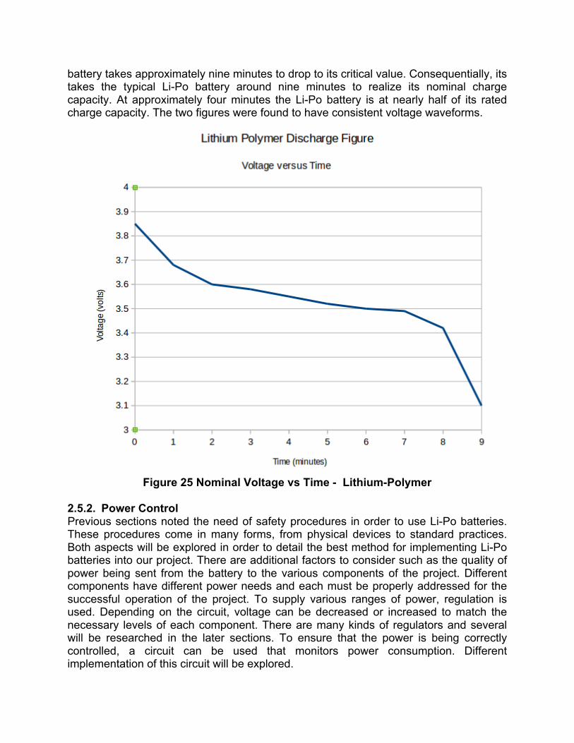
battery takes approximately nine minutes to drop to its critical value. Consequentially, its takes the typical Li-Po battery around nine minutes to realize its nominal charge capacity. At approximately four minutes the Li-Po battery is at nearly half of its rated charge capacity. The two figures were found to have consistent voltage waveforms.

Figure 25 Nominal Voltage vs Time - Lithium-Polymer

2.5.2. Power Control Previous sections noted the need of safety procedures in order to use Li-Po batteries. These procedures come in many forms, from physical devices to standard practices. Both aspects will be explored in order to detail the best method for implementing Li-Po batteries into our project. There are additional factors to consider such as the quality of power being sent from the battery to the various components of the project. Different components have different power needs and each must be properly addressed for the successful operation of the project. To supply various ranges of power, regulation is used. Depending on the circuit, voltage can be decreased or increased to match the necessary levels of each component. There are many kinds of regulators and several will be researched in the later sections. To ensure that the power is being correctly controlled, a circuit can be used that monitors power consumption. Different implementation of this circuit will be explored.

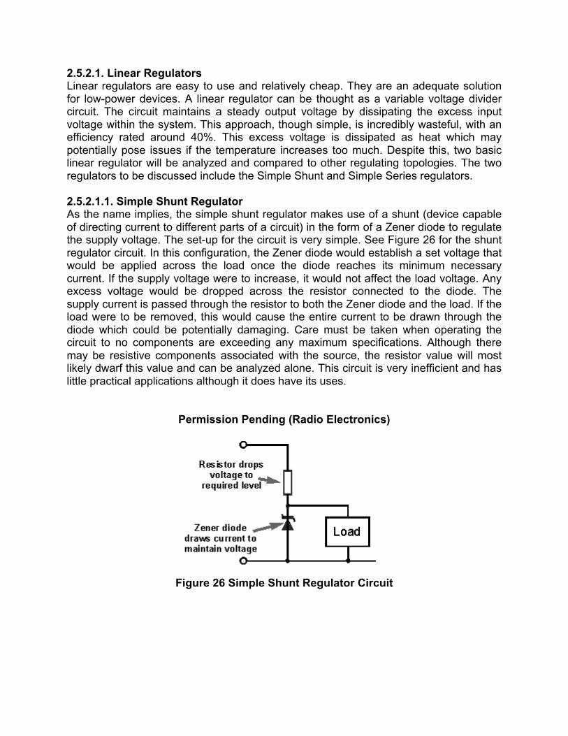
2.5.2.1. Linear Regulators Linear regulators are easy to use and relatively cheap. They are an adequate solution for low-power devices. A linear regulator can be thought as a variable voltage divider circuit. The circuit maintains a steady output voltage by dissipating the excess input voltage within the system. This approach, though simple, is incredibly wasteful, with an efficiency rated around 40%. This excess voltage is dissipated as heat which may potentially pose issues if the temperature increases too much. Despite this, two basic linear regulator will be analyzed and compared to other regulating topologies. The two regulators to be discussed include the Simple Shunt and Simple Series regulators. 2.5.2.1.1. Simple Shunt Regulator As the name implies, the simple shunt regulator makes use of a shunt (device capable of directing current to different parts of a circuit) in the form of a Zener diode to regulate the supply voltage. The set-up for the circuit is very simple. See Figure 26 for the shunt regulator circuit. In this configuration, the Zener diode would establish a set voltage that would be applied across the load once the diode reaches its minimum necessary current. If the supply voltage were to increase, it would not affect the load voltage. Any excess voltage would be dropped across the resistor connected to the diode. The supply current is passed through the resistor to both the Zener diode and the load. If the load were to be removed, this would cause the entire current to be drawn through the diode which could be potentially damaging. Care must be taken when operating the circuit to no components are exceeding any maximum specifications. Although there may be resistive components associated with the source, the resistor value will most likely dwarf this value and can be analyzed alone. This circuit is very inefficient and has little practical applications although it does have its uses.

Permission Pending (Radio Electronics)

Figure 26 Simple Shunt Regulator Circuit

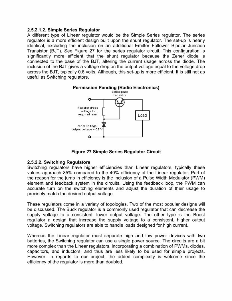
2.5.2.1.2. Simple Series Regulator A different type of Linear regulator would be the Simple Series regulator. The series regulator is a more efficient design built upon the shunt regulator. The set-up is nearly identical, excluding the inclusion on an additional Emitter Follower Bipolar Junction Transistor (BJT). See Figure 27 for the series regulator circuit. This configuration is significantly more efficient that the shunt regulator because the Zener diode is connected to the base of the BJT, altering the current usage across the diode. The inclusion of the BJT gives a voltage drop on the output voltage equal to the voltage drop across the BJT, typically 0.6 volts. Although, this set-up is more efficient. It is still not as useful as Switching regulators.

Permission Pending (Radio Electronics)

Figure 27 Simple Series Regulator Circuit 2.5.2.2. Switching Regulators Switching regulators have higher efficiencies than Linear regulators, typically these values approach 85% compared to the 40% efficiency of the Linear regulator. Part of the reason for the jump in efficiency is the inclusion of a Pulse Width Modulator (PWM) element and feedback system in the circuits. Using the feedback loop, the PWM can accurate turn on the switching elements and adjust the duration of their usage to precisely match the desired output voltage. These regulators come in a variety of topologies. Two of the most popular designs will be discussed. The Buck regulator is a commonly used regulator that can decrease the supply voltage to a consistent, lower output voltage. The other type is the Boost regulator a design that increase the supply voltage to a consistent, higher output voltage. Switching regulators are able to handle loads designed for high current. Whereas the Linear regulator must separate high and low power devices with two batteries, the Switching regulator can use a single power source. The circuits are a bit more complex than the Linear regulators, incorporating a combination of PWMs, diodes, capacitors, and inductors, and thus are less likely to be used for simple projects. However, in regards to our project, the added complexity is welcome since the efficiency of the regulator is more than doubled.

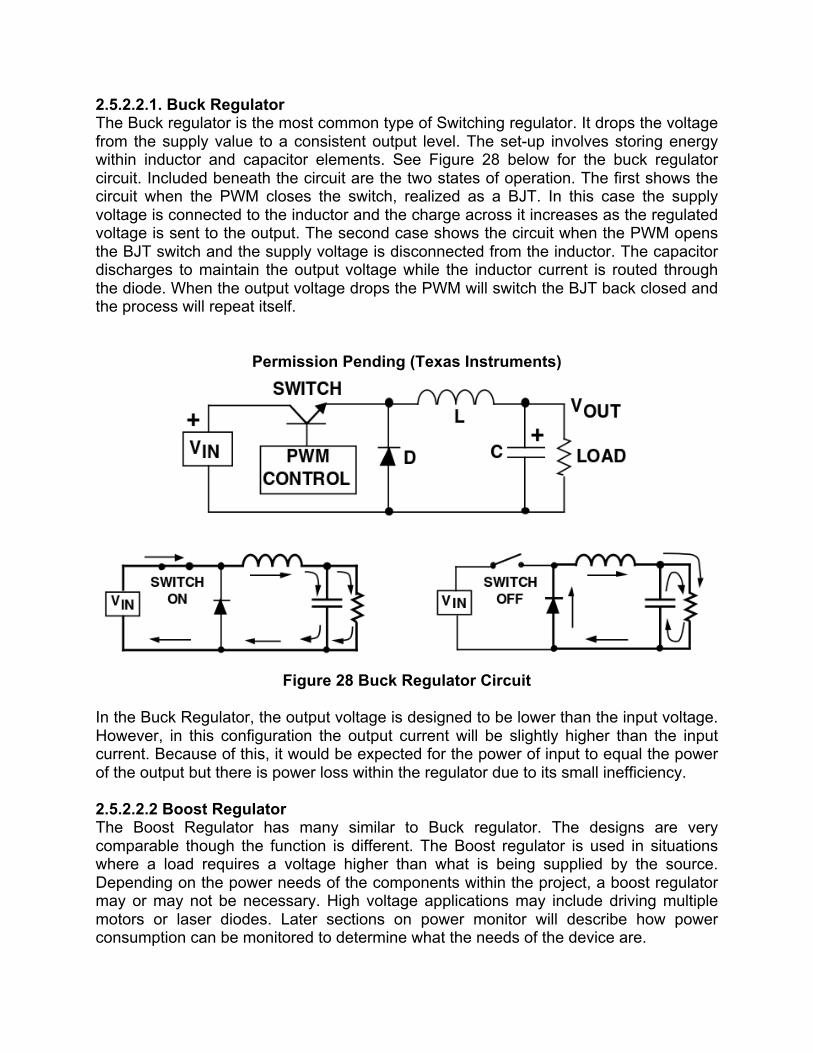
2.5.2.2.1. Buck Regulator The Buck regulator is the most common type of Switching regulator. It drops the voltage from the supply value to a consistent output level. The set-up involves storing energy within inductor and capacitor elements. See Figure 28 below for the buck regulator circuit. Included beneath the circuit are the two states of operation. The first shows the circuit when the PWM closes the switch, realized as a BJT. In this case the supply voltage is connected to the inductor and the charge across it increases as the regulated voltage is sent to the output. The second case shows the circuit when the PWM opens the BJT switch and the supply voltage is disconnected from the inductor. The capacitor discharges to maintain the output voltage while the inductor current is routed through the diode. When the output voltage drops the PWM will switch the BJT back closed and the process will repeat itself.

Permission Pending (Texas Instruments)

Figure 28 Buck Regulator Circuit

In the Buck Regulator, the output voltage is designed to be lower than the input voltage. However, in this configuration the output current will be slightly higher than the input current. Because of this, it would be expected for the power of input to equal the power of the output but there is power loss within the regulator due to its small inefficiency. 2.5.2.2.2 Boost Regulator The Boost Regulator has many similar to Buck regulator. The designs are very comparable though the function is different. The Boost regulator is used in situations where a load requires a voltage higher than what is being supplied by the source. Depending on the power needs of the components within the project, a boost regulator may or may not be necessary. High voltage applications may include driving multiple motors or laser diodes. Later sections on power monitor will describe how power consumption can be monitored to determine what the needs of the device are.

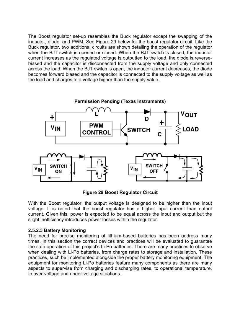
The Boost regulator set-up resembles the Buck regulator except the swapping of the inductor, diode, and PWM. See Figure 29 below for the boost regulator circuit. Like the Buck regulator, two additional circuits are shown detailing the operation of the regulator when the BJT switch is opened or closed. When the BJT switch is closed, the inductor current increases as the regulated voltage is outputted to the load, the diode is reverse-biased and the capacitor is disconnected from the supply voltage and only connected across the load. When the BJT switch is open, the inductor current decreases, the diode becomes forward biased and the capacitor is connected to the supply voltage as well as the load and charges to a voltage higher than the supply value.

Permission Pending (Texas Instruments)

Figure 29 Boost Regulator Circuit

With the Boost regulator, the output voltage is designed to be higher than the input voltage. It is noted that the boost regulator has a higher input current than output current. Given this, power is expected to be equal across the input and output but the slight inefficiency introduces power losses within the regulator. 2.5.2.3 Battery Monitoring The need for precise monitoring of lithium-based batteries has been address many times, in this section the correct devices and practices will be evaluated to guarantee the safe operation of this project’s Li-Po batteries. There are many practices to observe when dealing with Li-Po batteries, from charge rates to storage and installation. These practices, such be implemented alongside the proper battery monitoring equipment. The equipment for monitoring Li-Po batteries feature many components as there are many aspects to supervise from charging and discharging rates, to operational temperature, to over-voltage and under-voltage situations.

2.5.2.3.1 Safety Procedures for Li-Po Batteries There are different types of safety procedures for Li-Po batteries. It is important that they are observed because incorrectly used batteries are prone to catching fire or exploding. Among the set of safety guidelines there are a subset that distinctly concern proper operation. It deals with the charging and typical usage aspects of Li-Po batteries. Common safety guidelines include the follow recommendations: ● Do not charge the battery above the maximum rated voltage (typically 4.2V) ● Do not discharge the battery below the minimum rated voltage (typically 3.0V) ● Do not draw more than the rated capable current (typically 1 - 2�) ● Do not charge the battery with more than the rated capable current (typically 1�) ● Do not charge the battery beyond the rated temperature (typically 0 - 50�)

In addition to the procedures listed above, there are more general guidelines that focus on the building, testing and storage aspects of the Li-Po battery. These practices discuss how to care for the battery when it is not connected to a circuit. Common safety guidelines include the following recommendations: ● Do not immerse the battery in liquid ● Do not store the battery in heat ● Do not connect the battery with reversed polarity ● Do not discard the battery in fire ● Do not short-circuit the battery ● Do not apply a soldering iron to the battery or the terminals

Though it is not included in either of the guidelines, it is not considered a safe practice to connect Li-Po batteries in series or parallel. The reason for this is because there are minute differences in charge capacity and internal resistance that could result in connected batteries charging into one another and causing damage. There are noted alternatives for connecting batteries together. In many cases, a battery is wired in series in order to increase the supply voltage. Instead of connecting the batteries in series it is recommended to implement a step-up regulator such as the Boost regulator discussed in previous sections. Alternatively, batteries are often wired in parallel because the circuit designer wishes to increase the charge capacity. Instead of connecting multiple batteries together, it is recommended that the designer select a manufactured pack that supplies the desired charge capacity. These manufactured packs consist of multiple Li-Po batteries, however, they are safer for use because they were tested to have similar specifications can are not expected to discharge into one another. 2.5.2.3.2 Charge Controllers Charge controllers are devices used to limit the rate at which a battery can charge or discharge. Charge controllers are a vital component of the battery recharging process, as it prevents the battery from drawing too much current from the primary power source. By handling overcharging a charge controller may also prevent the possibility of over-voltages, though this situation will be explored on its own in later sections. There are

two different kinds of charge controllers. There are the simpler series and shunt charge controllers and there are the more robust designs that utilize Pulse Width Modulation (PWM) and Maximum Power Point Tracking (MPPT). The simple and complex variants somewhat resemble the design philosophies behind the Linear and Switching regulator. This is because the function of a charge controller is very similar to the function of a regulator. 2.5.2.3.2.1 Simple Charge Controllers The simple charge controllers use series and shunt designs to control the amount of charge that is supplied to the battery this is accomplished by measuring the battery’s voltage. When the battery voltage has not exceeded the limit, charge is allowed to freely flow into or out of the battery. However, when the limit has been exceeded. The battery stops being charged and the excess voltage is dropped across the charge controller. This is similar to the function of the Linear regulator and likewise these types of charge controllers have very poor efficiency. 2.5.2.3.2.2 Complex Charge Controllers The other type of charge controller makes use of a PWM and MPPT. It operates with three basic phases. The first phase is referred to as a bulk phase. During this phase, the voltage of the battery increases while the current being driven is very high. The next phase is called absorption in which the current supplied to the battery begins to drop off and battery voltage evens out near the maximum rated voltage. The final phase is the float phase where the battery is supplied as little current as possible to maintain the current battery voltage. Charge controllers may also include information regarding overheating and power monitoring, however, this varies among devices. If a particular charge controller does not have these features they can still be implemented in additional components. These additional components will be discussed further in later sections. 2.5.2.3.3 Protection Circuits When dealing with Li-Po batteries it is important to make a distinction between protected and ‘raw’ batteries. Protected batteries come from the manufacturer with a protection circuit attached to the battery cell. This protection circuit accomplishes the tasks that will be described within later sections. Raw batteries on the other hand, do not come with built-in protection circuits and are incredibly risky to use. It is possible to use external IC to achieve the same, safe functionality of protected batteries along more effort must be used to correctly set the conditions for the battery or else the battery is liable to catch fire or explode. There is another important distinction to make between Li-Po batteries. that is the one between regular Li-Po batteries and the Radio Control (RC) batteries. RC batteries are used in high-power devices such as UAVs and drones. These RC batteries are typical raw cells. RC batteries have a noticeably higher charge capability and thus are able to deliver power at incredibly fast rates ( up to 20 C ) though it is still recommended that the battery is not recharged at a rate higher than 1 C. Depending on the power

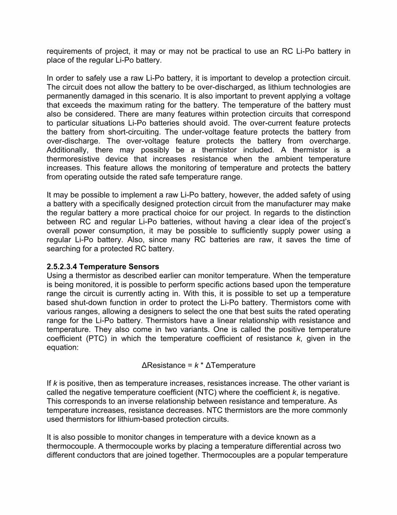
requirements of project, it may or may not be practical to use an RC Li-Po battery in place of the regular Li-Po battery. In order to safely use a raw Li-Po battery, it is important to develop a protection circuit. The circuit does not allow the battery to be over-discharged, as lithium technologies are permanently damaged in this scenario. It is also important to prevent applying a voltage that exceeds the maximum rating for the battery. The temperature of the battery must also be considered. There are many features within protection circuits that correspond to particular situations Li-Po batteries should avoid. The over-current feature protects the battery from short-circuiting. The under-voltage feature protects the battery from over-discharge. The over-voltage feature protects the battery from overcharge. Additionally, there may possibly be a thermistor included. A thermistor is a thermoresistive device that increases resistance when the ambient temperature increases. This feature allows the monitoring of temperature and protects the battery from operating outside the rated safe temperature range. It may be possible to implement a raw Li-Po battery, however, the added safety of using a battery with a specifically designed protection circuit from the manufacturer may make the regular battery a more practical choice for our project. In regards to the distinction between RC and regular Li-Po batteries, without having a clear idea of the project’s overall power consumption, it may be possible to sufficiently supply power using a regular Li-Po battery. Also, since many RC batteries are raw, it saves the time of searching for a protected RC battery. 2.5.2.3.4 Temperature Sensors Using a thermistor as described earlier can monitor temperature. When the temperature is being monitored, it is possible to perform specific actions based upon the temperature range the circuit is currently acting in. With this, it is possible to set up a temperature based shut-down function in order to protect the Li-Po battery. Thermistors come with various ranges, allowing a designers to select the one that best suits the rated operating range for the Li-Po battery. Thermistors have a linear relationship with resistance and temperature. They also come in two variants. One is called the positive temperature coefficient (PTC) in which the temperature coefficient of resistance k, given in the equation:

ΔResistance = k * ΔTemperature

If k is positive, then as temperature increases, resistances increase. The other variant is called the negative temperature coefficient (NTC) where the coefficient k, is negative. This corresponds to an inverse relationship between resistance and temperature. As temperature increases, resistance decreases. NTC thermistors are the more commonly used thermistors for lithium-based protection circuits. It is also possible to monitor changes in temperature with a device known as a thermocouple. A thermocouple works by placing a temperature differential across two different conductors that are joined together. Thermocouples are a popular temperature

sensing device and are capable of monitoring and manipulating a system based on the measured temperature. Thermocouples use a slightly more complex equation in order to derive the change in temperature. The equation, which utilizes the Seebeck effect is as given:

� Voltage = --( Seebeck Coefficient ) * ∇ Temperature

where the ∇ signifies a gradient operation. In a broad sense, a gradient gives the slope, or change, of a function in multiple dimensions. Given that, the equation for the thermocouple is very similar to the equation for the thermistor. In regards for picking either a thermistor or a thermocouple, the thermistor is a more popular selection for the task of monitoring Li-Po batteries and has a slightly smaller form-factor. Regardless of which device is used, the temperature of the Li-Po battery should remain within 0 – 50 V. 2.5.2.3.5 Over-voltage Control For the Li-Po battery to function properly, the cell should not be charged to a voltage that exceeds the maximum rating. There are many approaches to prevent this from occurring.To safely operate the Li-Po batttery there should be a safety cut-off set for 4.2 V. This limit would protect the battery from overcharging and potentially being damaged. This can be achieved through manufactured protection circuits, specialized protection IC’s, or through the usage of simple or complex charge controllers. 2.5.2.3.6 Under-voltage Control While over-voltage is being control, it is also important to make sure the Li-Po is not being over-discharged. This situation is very crucial as an over-discharge could permanently damage the Li-Po battery and leave it unusable. To safely operate the Li-Po battery there should be a safety cut-off set for 3.0 V. This factor can also be monitored with manufactured protection circuits, external protection IC’s or charge controllers. 2.5.2.4 Power Monitoring (INA219) With the vast number of components running within our project, it is difficult to estimate an overall power usage. In this situation, using a separate circuit to accomplish this task is ideal. This circuit can be may for instance be realized with one particular IC, the INA219, which measures voltage and high side current of design and sends the power usage over I2C. This allows our group to get a detailed look at how power is being consumed in case any changes need to be made with how power is supplied or how long are battery is capable of lasting. There are other methods that can produce the same result. The intention is to develop a reliable estimation of overall power consumption which allow values for components such as the regulator and battery to be determined.

2.7 Data Interpretation Software Gathering all of the data from this device is one thing, but it all means nothing unless the data can be interpreted. There are several ways we could go about interpreting the data, but we want to focus on a more user-friendly approach that provides a visually appealing representation of the data we obtain from scanning an environment. One way of interpreting and representing the data in this manner is by using a point cloud. 2.7.1 Point Cloud Point clouds are sets of data points within a coordinate system. In a three-dimensional coordinate system, the sets of data are used to represent the surface of an object. The data points are the points measured by the lidar system. A point cloud will be formed from the data points that are measured. In order to accurately represent this data, the point cloud library will be used. The Point Cloud Library is an open-source library that is used to create and interpret point cloud data. It will help to manipulate the data to fit the needs of our goals. The point cloud library contains several algorithms for processing point clouds. These include filtering, feature estimation, and surface recognition to name a few. By using the algorithms provided by the point cloud library, we will be able to filter noise, create surfaces, and extract the important points to represent objects based on their geometric appearance. One library we will use to capture the point clouds from our device is the pcl_io library. It contains classes and functions that can read and write point cloud data. This library will help us to manipulate the changing point cloud based on the new data coming in from each scan of the environment. Another library that we will be using to help to create a visualization of the point clouds is the pcl_range_image library. A range image is an image of pixelated values that represent distances. These distances are measured from the range finding module’s origin. This library contains classes that not only represent a range image based on the point cloud data, but also manipulate the range images. The pcl_visualization library will also be used to create a visualization of the data. This library allows for prototyping and visualizing the results of the algorithms that were used to interpret three-dimensional point cloud data. It contains methods for rendering and setting visual properties to the point cloud data. These visual properties include color, opacity, and point size. It also contains methods to draw three-dimensional shapes on screen based on data sets. This library will help to visualize the data gathered from the environment that is being scanned. 2.7.2 Computer Vision Computer vision is a way of processing and analyzing images and data in order to produce numerical data. It creates 3D models from image data. Our data is interpreted and represented in real-time, computer vision is highly effective for our project.

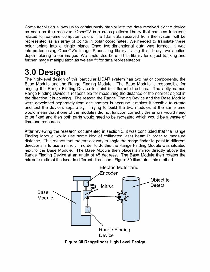
Computer vision allows us to continuously manipulate the data received by the device as soon as it is received. OpenCV is a cross-platform library that contains functions related to real-time computer vision. The lidar data received from the system will be represented as an array of points in polar coordinates. We needed to translate these polar points into a single plane. Once two-dimensional data was formed, it was interpreted using OpenCV’s Image Processing library. Using this library, we applied depth coloring to our images. We could also be use this library for object tracking and further image manipulation as we see fit for data representation.

3.0 Design The high-level design of this particular LIDAR system has two major components, the Base Module and the Range Finding Module. The Base Module is responsible for angling the Range Finding Device to point in different directions. The aptly named Range Finding Device is responsible for measuring the distance of the nearest object in the direction it is pointing. The reason the Range Finding Device and the Base Module were developed separately from one another is because it makes it possible to create and test the devices separately. Trying to build the two modules at the same time would mean that if one of the modules did not function correctly the errors would need to be fixed and then both parts would need to be recreated which would be a waste of time and resources. After reviewing the research documented in section 2, it was concluded that the Range Finding Module would use some kind of collimated laser beam in order to measure distance. This means that the easiest way to angle the range finder to point in different directions is to use a mirror. In order to do this the Range Finding Module was situated next to the Base Module. The Base Module then places a mirror directly above the Range Finding Device at an angle of 45 degrees. The Base Module then rotates the mirror to redirect the laser in different directions. Figure 30 illustrates this method.

Figure 30 Rangefinder High Level Design

Mirror

Electric Motor and Encoder

Range Finding Device

Base Module

Object to Detect

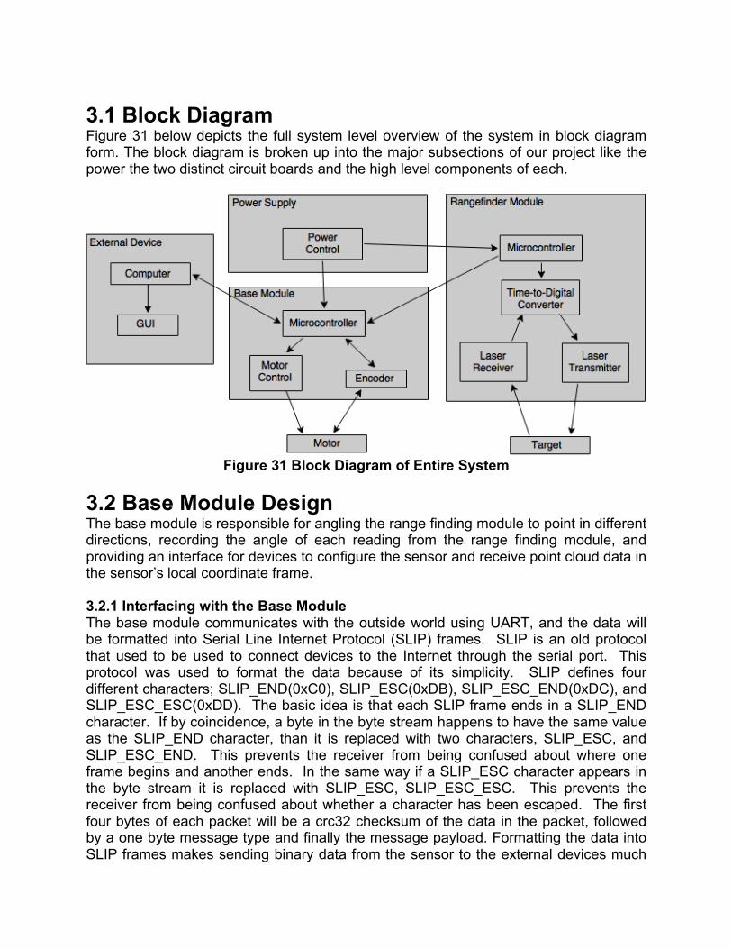
3.1 Block Diagram Figure 31 below depicts the full system level overview of the system in block diagram form. The block diagram is broken up into the major subsections of our project like the power the two distinct circuit boards and the high level components of each.

Figure 31 Block Diagram of Entire System

3.2 Base Module Design The base module is responsible for angling the range finding module to point in different directions, recording the angle of each reading from the range finding module, and providing an interface for devices to configure the sensor and receive point cloud data in the sensor’s local coordinate frame. 3.2.1 Interfacing with the Base Module The base module communicates with the outside world using UART, and the data will be formatted into Serial Line Internet Protocol (SLIP) frames. SLIP is an old protocol that used to be used to connect devices to the Internet through the serial port. This protocol was used to format the data because of its simplicity. SLIP defines four different characters; SLIP_END(0xC0), SLIP_ESC(0xDB), SLIP_ESC_END(0xDC), and SLIP_ESC_ESC(0xDD). The basic idea is that each SLIP frame ends in a SLIP_END character. If by coincidence, a byte in the byte stream happens to have the same value as the SLIP_END character, than it is replaced with two characters, SLIP_ESC, and SLIP_ESC_END. This prevents the receiver from being confused about where one frame begins and another ends. In the same way if a SLIP_ESC character appears in the byte stream it is replaced with SLIP_ESC, SLIP_ESC_ESC. This prevents the receiver from being confused about whether a character has been escaped. The first four bytes of each packet will be a crc32 checksum of the data in the packet, followed by a one byte message type and finally the message payload. Formatting the data into SLIP frames makes sending binary data from the sensor to the external devices much

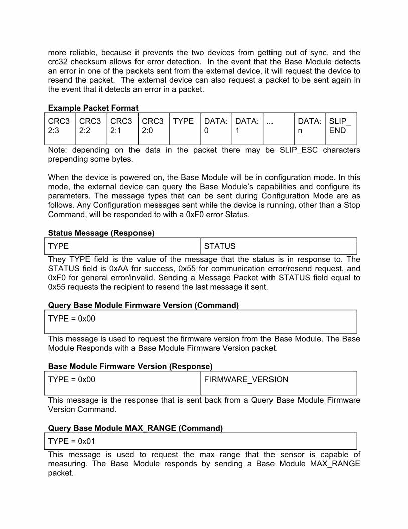
more reliable, because it prevents the two devices from getting out of sync, and the crc32 checksum allows for error detection. In the event that the Base Module detects an error in one of the packets sent from the external device, it will request the device to resend the packet. The external device can also request a packet to be sent again in the event that it detects an error in a packet. Example Packet Format CRC32:3

CRC32:2

CRC32:1

CRC32:0

TYPE DATA:0

DATA:1

... DATA:n

SLIP_END

Note: depending on the data in the packet there may be SLIP_ESC characters prepending some bytes. When the device is powered on, the Base Module will be in configuration mode. In this mode, the external device can query the Base Module’s capabilities and configure its parameters. The message types that can be sent during Configuration Mode are as follows. Any Configuration messages sent while the device is running, other than a Stop Command, will be responded to with a 0xF0 error Status. Status Message (Response) TYPE STATUS They TYPE field is the value of the message that the status is in response to. The STATUS field is 0xAA for success, 0x55 for communication error/resend request, and 0xF0 for general error/invalid. Sending a Message Packet with STATUS field equal to 0x55 requests the recipient to resend the last message it sent. Query Base Module Firmware Version (Command) TYPE = 0x00

This message is used to request the firmware version from the Base Module. The Base Module Responds with a Base Module Firmware Version packet. Base Module Firmware Version (Response) TYPE = 0x00 FIRMWARE_VERSION

This message is the response that is sent back from a Query Base Module Firmware Version Command. Query Base Module MAX_RANGE (Command) TYPE = 0x01 This message is used to request the max range that the sensor is capable of measuring. The Base Module responds by sending a Base Module MAX_RANGE packet.

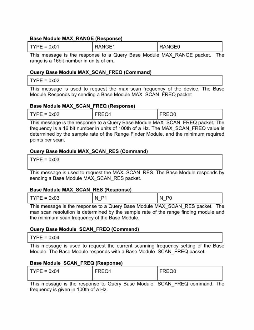
Base Module MAX_RANGE (Response) TYPE = 0x01 RANGE1 RANGE0 This message is the response to a Query Base Module MAX_RANGE packet. The range is a 16bit number in units of cm. Query Base Module MAX_SCAN_FREQ (Command) TYPE = 0x02 This message is used to request the max scan frequency of the device. The Base Module Responds by sending a Base Module MAX_SCAN_FREQ packet Base Module MAX_SCAN_FREQ (Response) TYPE = 0x02 FREQ1 FREQ0 This message is the response to a Query Base Module MAX_SCAN_FREQ packet. The frequency is a 16 bit number in units of 100th of a Hz. The MAX_SCAN_FREQ value is determined by the sample rate of the Range Finder Module, and the minimum required points per scan. Query Base Module MAX_SCAN_RES (Command) TYPE = 0x03

This message is used to request the MAX_SCAN_RES. The Base Module responds by sending a Base Module MAX_SCAN_RES packet. Base Module MAX_SCAN_RES (Response) TYPE = 0x03 N_P1 N_P0 This message is the response to a Query Base Module MAX_SCAN_RES packet. The max scan resolution is determined by the sample rate of the range finding module and the minimum scan frequency of the Base Module. Query Base Module SCAN_FREQ (Command) TYPE = 0x04 This message is used to request the current scanning frequency setting of the Base Module. The Base Module responds with a Base Module SCAN_FREQ packet. Base Module SCAN_FREQ (Response) TYPE = 0x04 FREQ1 FREQ0

This message is the response to Query Base Module SCAN_FREQ command. The frequency is given in 100th of a Hz.

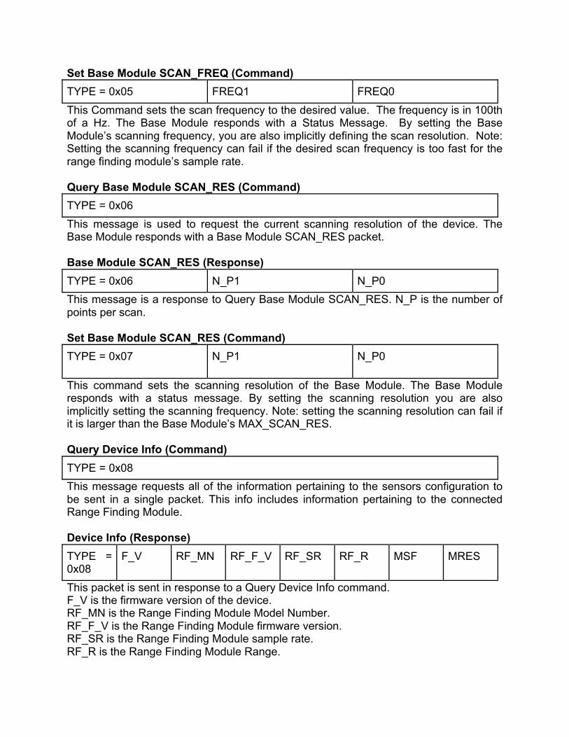
Set Base Module SCAN_FREQ (Command) TYPE = 0x05 FREQ1 FREQ0 This Command sets the scan frequency to the desired value. The frequency is in 100th of a Hz. The Base Module responds with a Status Message. By setting the Base Module’s scanning frequency, you are also implicitly defining the scan resolution. Note: Setting the scanning frequency can fail if the desired scan frequency is too fast for the range finding module’s sample rate. Query Base Module SCAN_RES (Command) TYPE = 0x06 This message is used to request the current scanning resolution of the device. The Base Module responds with a Base Module SCAN_RES packet. Base Module SCAN_RES (Response) TYPE = 0x06 N_P1 N_P0 This message is a response to Query Base Module SCAN_RES. N_P is the number of points per scan. Set Base Module SCAN_RES (Command) TYPE = 0x07 N_P1 N_P0

This command sets the scanning resolution of the Base Module. The Base Module responds with a status message. By setting the scanning resolution you are also implicitly setting the scanning frequency. Note: setting the scanning resolution can fail if it is larger than the Base Module’s MAX_SCAN_RES. Query Device Info (Command) TYPE = 0x08 This message requests all of the information pertaining to the sensors configuration to be sent in a single packet. This info includes information pertaining to the connected Range Finding Module. Device Info (Response) TYPE = 0x08

F_V RF_MN RF_F_V RF_SR RF_R MSF MRES

This packet is sent in response to a Query Device Info command. F_V is the firmware version of the device. RF_MN is the Range Finding Module Model Number. RF_F_V is the Range Finding Module firmware version. RF_SR is the Range Finding Module sample rate. RF_R is the Range Finding Module Range.

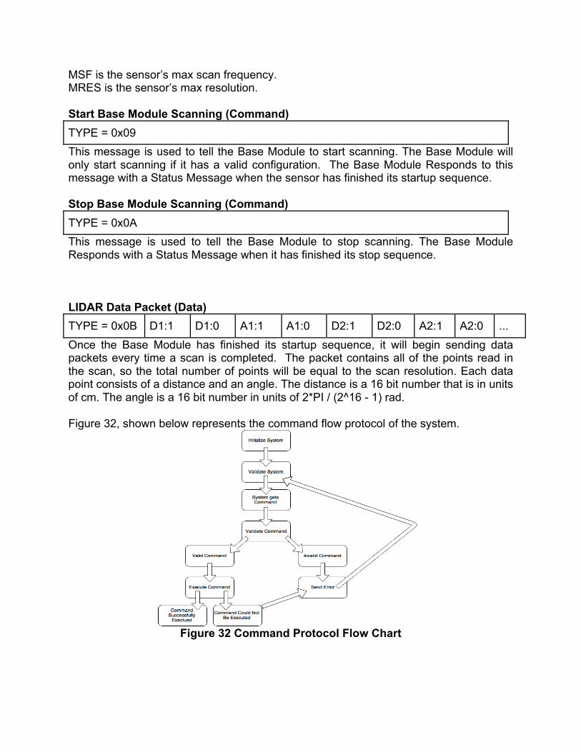
MSF is the sensor’s max scan frequency. MRES is the sensor’s max resolution. Start Base Module Scanning (Command) TYPE = 0x09 This message is used to tell the Base Module to start scanning. The Base Module will only start scanning if it has a valid configuration. The Base Module Responds to this message with a Status Message when the sensor has finished its startup sequence. Stop Base Module Scanning (Command) TYPE = 0x0A This message is used to tell the Base Module to stop scanning. The Base Module Responds with a Status Message when it has finished its stop sequence. LIDAR Data Packet (Data) TYPE = 0x0B D1:1 D1:0 A1:1 A1:0 D2:1 D2:0 A2:1 A2:0 ... Once the Base Module has finished its startup sequence, it will begin sending data packets every time a scan is completed. The packet contains all of the points read in the scan, so the total number of points will be equal to the scan resolution. Each data point consists of a distance and an angle. The distance is a 16 bit number that is in units of cm. The angle is a 16 bit number in units of 2*PI / (2^16 - 1) rad. Figure 32, shown below represents the command flow protocol of the system.

Figure 32 Command Protocol Flow Chart

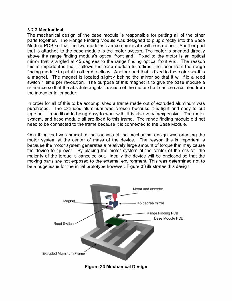
3.2.2 Mechanical The mechanical design of the base module is responsible for putting all of the other parts together. The Range Finding Module was designed to plug directly into the Base Module PCB so that the two modules can communicate with each other. Another part that is attached to the base module is the motor system. The motor is oriented directly above the range finding module’s optical front end. Fixed to the motor is an optical mirror that is angled at 45 degrees to the range finding optical front end. The reason this is important is that it allows the base module to redirect the laser from the range finding module to point in other directions. Another part that is fixed to the motor shaft is a magnet. The magnet is located slightly behind the mirror so that it will flip a reed switch 1 time per revolution. The purpose of this magnet is to give the base module a reference so that the absolute angular position of the motor shaft can be calculated from the incremental encoder. In order for all of this to be accomplished a frame made out of extruded aluminum was purchased. The extruded aluminum was chosen because it is light and easy to put together. In addition to being easy to work with, it is also very inexpensive. The motor system, and base module all are fixed to this frame. The range finding module did not need to be connected to the frame because it is connected to the Base Module. One thing that was crucial to the success of the mechanical design was orienting the motor system at the center of mass of the device. The reason this is important is because the motor system generates a relatively large amount of torque that may cause the device to tip over. By placing the motor system at the center of the device, the majority of the torque is canceled out. Ideally the device will be enclosed so that the moving parts are not exposed to the external environment. This was determined not to be a huge issue for the initial prototype however. Figure 33 illustrates this design.

Figure 33 Mechanical Design

The device is designed to be able to bolt down on to a mounting system so that it can be used in other designs. For demonstration purposes the device was mounted to a heavy weight so that it will not tip over because of the torque created by the moving parts. This fixture also holds a LiPo battery for powering the device without a power supply. 3.2.3 Electrical The electrical configuration for the base module is not near as in-depth as the electrical configuration for the rangefinder module. The base module only consists of the power supplied to it, the motor control and encoder, and most importantly the microcontroller. The next section describes the specific functions of the base module’s microcontroller. 3.2.3.1 Microcontroller The Base Module needs a microcontroller in order to control the electric motor, reading the motor encoder, and getting range data from the Range Finding Module. None of these tasks require that much processing power. Any amount of power that the microcontroller is going to be negligible in comparison to the power usage of the electric motor. This means that just about any microcontroller will work for this module. If any microcontroller will work then it makes the most sense to select the one that costs the least. This design is just a prototype however, so the microcontroller that was chosen for this module was the same as the one chosen for the Range Finding Module. Choosing the same microcontroller for both modules make developing the firmware take much less time. For example, if both microcontrollers are the same, than all of the code for communication can be used in both projects. The microcontroller that was selected for the Range Finding Module was the STM32F407 32-bit ARM Cortex M4 MCU manufactured by STMicroelectronics. For a detailed analysis of why this microcontroller was selected see section 3.3.3.1. 3.2.4 Software The software used for the Base Module was all written in C/C++. The reason is because the software is running on an arm cortex-m4 microcontroller manufactured by STMicroelectronics. The particular chip chosen was an stm32f407 microcontroller. The most supported language for programming these microcontrollers is C/C++. The only other option for programming languages is assembly. In today’s world, programming in assembly is almost never recommended. The reason it is so frowned upon in industry, is because not only is it difficult to code in, but it also cannot be ported to other devices. By using C/C++ and by following good programming practices, the code is guaranteed to be portable to many different platforms. In order to be able to reuse code, it is important to have a general software architecture that is followed for every part of the project. For the code to be portable to many different environments it needs to have many abstraction layers. There are four abstraction layers in this particular design. The first and lowest layer is the hardware abstraction layer (HAL). This layer contains all of the microcontroller specific code including the port specific code for the RTOS (Realtime Operating System) Kernel, and

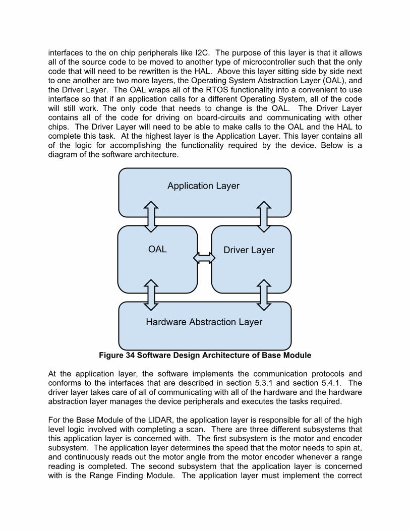
interfaces to the on chip peripherals like I2C. The purpose of this layer is that it allows all of the source code to be moved to another type of microcontroller such that the only code that will need to be rewritten is the HAL. Above this layer sitting side by side next to one another are two more layers, the Operating System Abstraction Layer (OAL), and the Driver Layer. The OAL wraps all of the RTOS functionality into a convenient to use interface so that if an application calls for a different Operating System, all of the code will still work. The only code that needs to change is the OAL. The Driver Layer contains all of the code for driving on board-circuits and communicating with other chips. The Driver Layer will need to be able to make calls to the OAL and the HAL to complete this task. At the highest layer is the Application Layer. This layer contains all of the logic for accomplishing the functionality required by the device. Below is a diagram of the software architecture.

Figure 34 Software Design Architecture of Base Module

At the application layer, the software implements the communication protocols and conforms to the interfaces that are described in section 5.3.1 and section 5.4.1. The driver layer takes care of all of communicating with all of the hardware and the hardware abstraction layer manages the device peripherals and executes the tasks required. For the Base Module of the LIDAR, the application layer is responsible for all of the high level logic involved with completing a scan. There are three different subsystems that this application layer is concerned with. The first subsystem is the motor and encoder subsystem. The application layer determines the speed that the motor needs to spin at, and continuously reads out the motor angle from the motor encoder whenever a range reading is completed. The second subsystem that the application layer is concerned with is the Range Finding Module. The application layer must implement the correct

Application Layer

OAL Driver Layer

Hardware Abstraction Layer

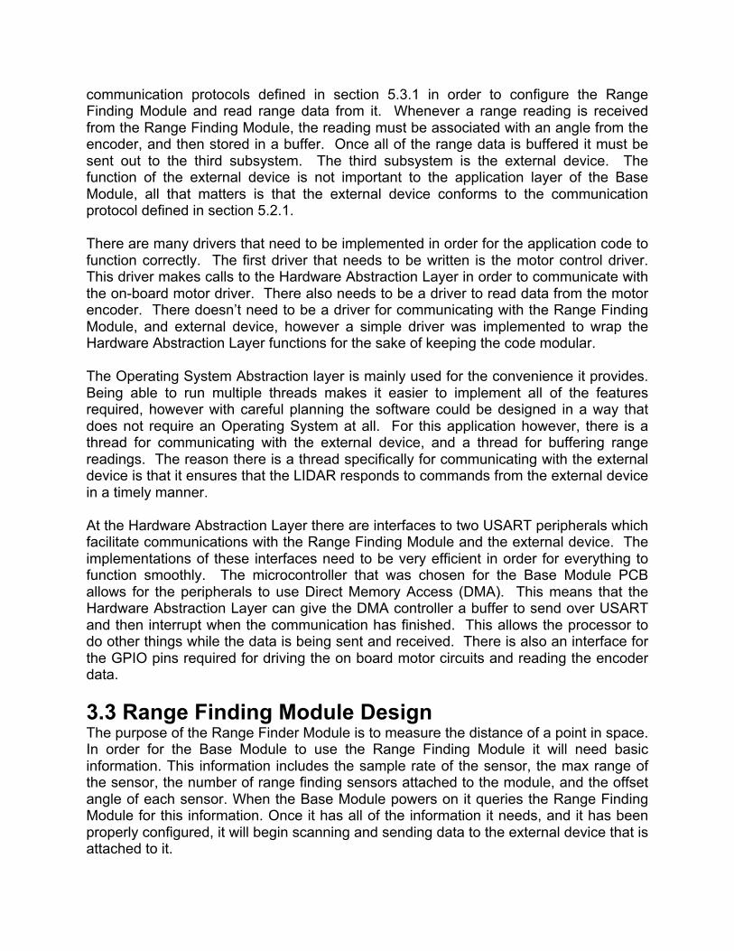
communication protocols defined in section 5.3.1 in order to configure the Range Finding Module and read range data from it. Whenever a range reading is received from the Range Finding Module, the reading must be associated with an angle from the encoder, and then stored in a buffer. Once all of the range data is buffered it must be sent out to the third subsystem. The third subsystem is the external device. The function of the external device is not important to the application layer of the Base Module, all that matters is that the external device conforms to the communication protocol defined in section 5.2.1. There are many drivers that need to be implemented in order for the application code to function correctly. The first driver that needs to be written is the motor control driver. This driver makes calls to the Hardware Abstraction Layer in order to communicate with the on-board motor driver. There also needs to be a driver to read data from the motor encoder. There doesn’t need to be a driver for communicating with the Range Finding Module, and external device, however a simple driver was implemented to wrap the Hardware Abstraction Layer functions for the sake of keeping the code modular. The Operating System Abstraction layer is mainly used for the convenience it provides. Being able to run multiple threads makes it easier to implement all of the features required, however with careful planning the software could be designed in a way that does not require an Operating System at all. For this application however, there is a thread for communicating with the external device, and a thread for buffering range readings. The reason there is a thread specifically for communicating with the external device is that it ensures that the LIDAR responds to commands from the external device in a timely manner. At the Hardware Abstraction Layer there are interfaces to two USART peripherals which facilitate communications with the Range Finding Module and the external device. The implementations of these interfaces need to be very efficient in order for everything to function smoothly. The microcontroller that was chosen for the Base Module PCB allows for the peripherals to use Direct Memory Access (DMA). This means that the Hardware Abstraction Layer can give the DMA controller a buffer to send over USART and then interrupt when the communication has finished. This allows the processor to do other things while the data is being sent and received. There is also an interface for the GPIO pins required for driving the on board motor circuits and reading the encoder data. 3.3 Range Finding Module Design The purpose of the Range Finder Module is to measure the distance of a point in space. In order for the Base Module to use the Range Finding Module it will need basic information. This information includes the sample rate of the sensor, the max range of the sensor, the number of range finding sensors attached to the module, and the offset angle of each sensor. When the Base Module powers on it queries the Range Finding Module for this information. Once it has all of the information it needs, and it has been properly configured, it will begin scanning and sending data to the external device that is attached to it.

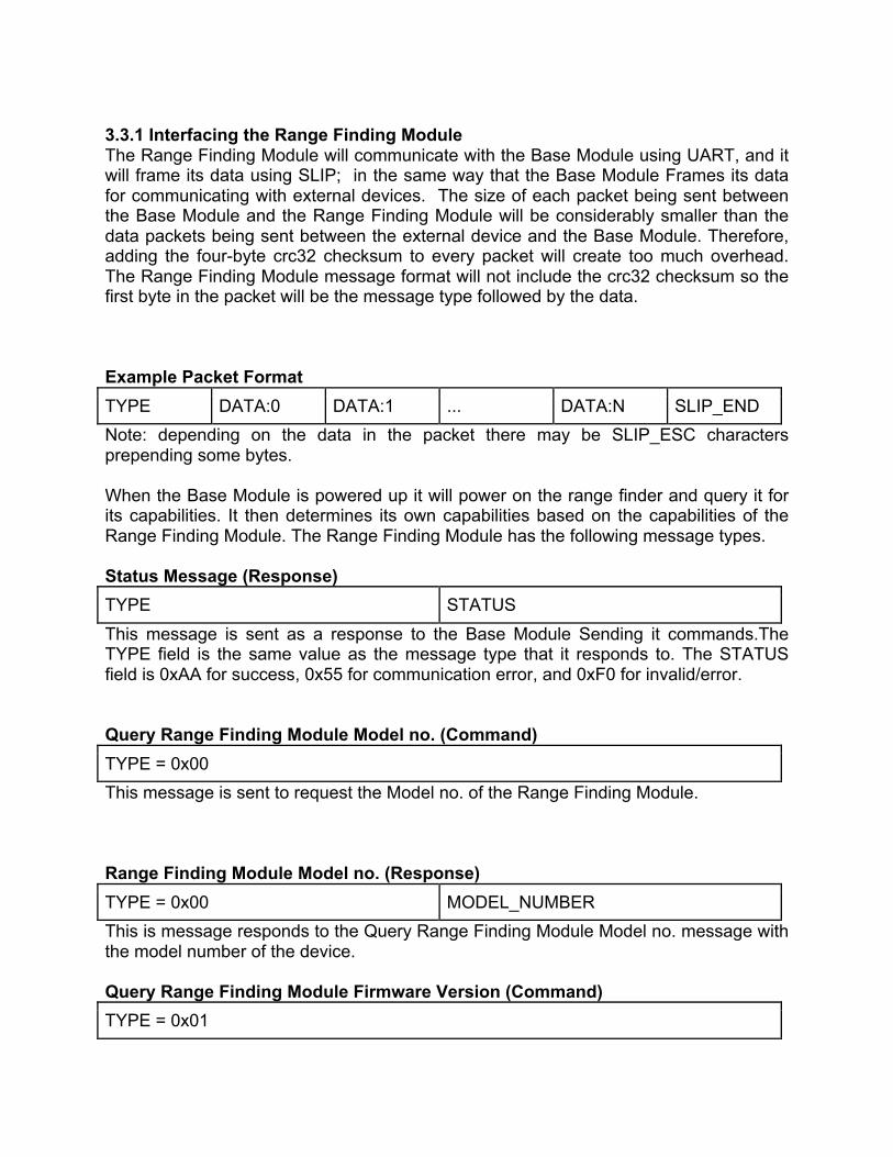
3.3.1 Interfacing the Range Finding Module The Range Finding Module will communicate with the Base Module using UART, and it will frame its data using SLIP; in the same way that the Base Module Frames its data for communicating with external devices. The size of each packet being sent between the Base Module and the Range Finding Module will be considerably smaller than the data packets being sent between the external device and the Base Module. Therefore, adding the four-byte crc32 checksum to every packet will create too much overhead. The Range Finding Module message format will not include the crc32 checksum so the first byte in the packet will be the message type followed by the data. Example Packet Format TYPE DATA:0 DATA:1 ... DATA:N SLIP_END Note: depending on the data in the packet there may be SLIP_ESC characters prepending some bytes. When the Base Module is powered up it will power on the range finder and query it for its capabilities. It then determines its own capabilities based on the capabilities of the Range Finding Module. The Range Finding Module has the following message types. Status Message (Response) TYPE STATUS This message is sent as a response to the Base Module Sending it commands.The TYPE field is the same value as the message type that it responds to. The STATUS field is 0xAA for success, 0x55 for communication error, and 0xF0 for invalid/error. Query Range Finding Module Model no. (Command) TYPE = 0x00 This message is sent to request the Model no. of the Range Finding Module. Range Finding Module Model no. (Response) TYPE = 0x00 MODEL_NUMBER This is message responds to the Query Range Finding Module Model no. message with the model number of the device. Query Range Finding Module Firmware Version (Command) TYPE = 0x01

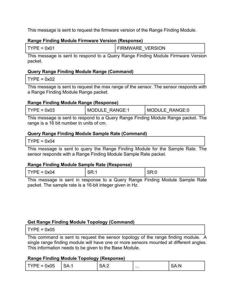
This message is sent to request the firmware version of the Range Finding Module. Range Finding Module Firmware Version (Response) TYPE = 0x01 FIRMWARE_VERSION This message is sent to respond to a Query Range Finding Module Firmware Version packet. Query Range Finding Module Range (Command) TYPE = 0x02 This message is sent to request the max range of the sensor. The sensor responds with a Range Finding Module Range packet. Range Finding Module Range (Response) TYPE = 0x03 MODULE_RANGE:1 MODULE_RANGE:0 This message is sent to respond to a Query Range Finding Module Range packet. The range is a 16 bit number in units of cm. Query Range Finding Module Sample Rate (Command) TYPE = 0x04 This message is sent to query the Range Finding Module for the Sample Rate. The sensor responds with a Range Finding Module Sample Rate packet. Range Finding Module Sample Rate (Response) TYPE = 0x04 SR:1 SR:0 This message is sent in response to a Query Range Finding Module Sample Rate packet. The sample rate is a 16-bit integer given in Hz. Get Range Finding Module Topology (Command) TYPE = 0x05 This command is sent to request the sensor topology of the range finding module. A single range finding module will have one or more sensors mounted at different angles. This information needs to be given to the Base Module. Range Finding Module Topology (Response) TYPE = 0x05 SA:1 SA:2 ... SA:N

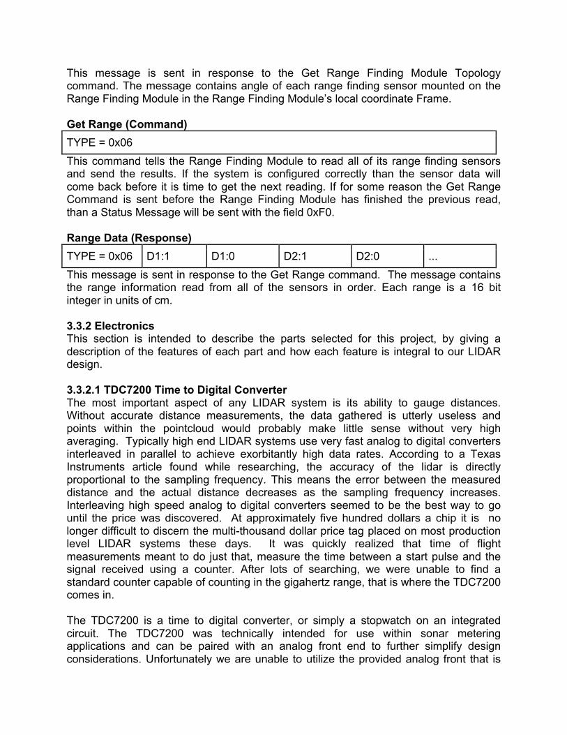
This message is sent in response to the Get Range Finding Module Topology command. The message contains angle of each range finding sensor mounted on the Range Finding Module in the Range Finding Module’s local coordinate Frame. Get Range (Command) TYPE = 0x06 This command tells the Range Finding Module to read all of its range finding sensors and send the results. If the system is configured correctly than the sensor data will come back before it is time to get the next reading. If for some reason the Get Range Command is sent before the Range Finding Module has finished the previous read, than a Status Message will be sent with the field 0xF0. Range Data (Response) TYPE = 0x06 D1:1 D1:0 D2:1 D2:0 ... This message is sent in response to the Get Range command. The message contains the range information read from all of the sensors in order. Each range is a 16 bit integer in units of cm. 3.3.2 Electronics This section is intended to describe the parts selected for this project, by giving a description of the features of each part and how each feature is integral to our LIDAR design. 3.3.2.1 TDC7200 Time to Digital Converter The most important aspect of any LIDAR system is its ability to gauge distances. Without accurate distance measurements, the data gathered is utterly useless and points within the pointcloud would probably make little sense without very high averaging. Typically high end LIDAR systems use very fast analog to digital converters interleaved in parallel to achieve exorbitantly high data rates. According to a Texas Instruments article found while researching, the accuracy of the lidar is directly proportional to the sampling frequency. This means the error between the measured distance and the actual distance decreases as the sampling frequency increases. Interleaving high speed analog to digital converters seemed to be the best way to go until the price was discovered. At approximately five hundred dollars a chip it is no longer difficult to discern the multi-thousand dollar price tag placed on most production level LIDAR systems these days. It was quickly realized that time of flight measurements meant to do just that, measure the time between a start pulse and the signal received using a counter. After lots of searching, we were unable to find a standard counter capable of counting in the gigahertz range, that is where the TDC7200 comes in. The TDC7200 is a time to digital converter, or simply a stopwatch on an integrated circuit. The TDC7200 was technically intended for use within sonar metering applications and can be paired with an analog front end to further simplify design considerations. Unfortunately we are unable to utilize the provided analog front that is

used in sonar applications, because it does not match well with our laser application. The TDC7200 does, however, give us a counting resolution of 55 picoseconds and a standard deviation of 35 picoseconds, allowing us to make measurements from 12 nanoseconds to 500 nanoseconds from the time of the start pulse. The device also has an internal self-calibrated time base, allowing it to correct drift over temperature over time. The internal time base is calibrated by an external clock operating on the order of megahertz. The external clock needs to be as accurate and stable as possible as all measurement accuracy is heavily dependant on the external clock accuracy. The external clock is also utilized by all digital circuitry within the TDC7200. The standard deviation of a set of measurement results, or the accuracy of the measurement results are proportional to the external reference clock, at a one megahertz reference clock the standard deviation is 243 picoseconds, this value decreases as shown in Figure 35 below. The figure shows that it is possible to achieve greater accuracy than the given 35 picoseconds standard deviation by increasing the external clock toward 16 megahertz.

Courtesy of Texas Instruments, inc.

Figure 35 Measurement deviation VS clock period

As noted in the previous section, the external clock is crucial to the accuracy of the TDC7200, or any other time sensitive device. The two most important factors to consider when selecting an external clock for use within time sensitive devices are the clock accuracy and the clock jitter. First of all, clock accuracy is the amount of deviation that the clock can vary from its nominally stated frequency, this deviation is measured in parts per million or PPM. Obviously a lower number is prefered over a larger number. For an example, if we were to use an 8 megahertz clock and our clock has a 20 PPM value. The actual frequency of the clock has an error value of plus or minus 20PPM, and the resulting frequency is between 7.99984 megahertz and 8.00016 megahertz or [8MHZ ± (8MHZ) x (20/1000000)]. For our project 20PPM or less will yield sufficient accuracy for the measurements we are performing. The second parameter responsible

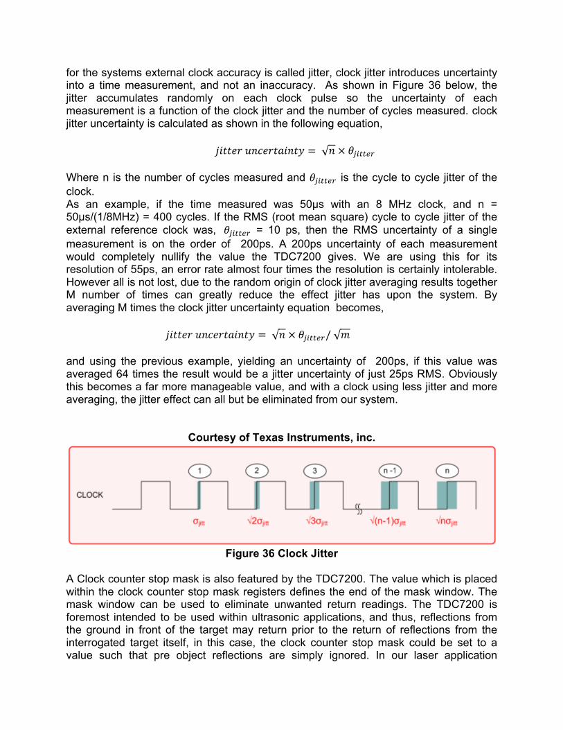
for the systems external clock accuracy is called jitter, clock jitter introduces uncertainty into a time measurement, and not an inaccuracy. As shown in Figure 36 below, the jitter accumulates randomly on each clock pulse so the uncertainty of each measurement is a function of the clock jitter and the number of cycles measured. clock jitter uncertainty is calculated as shown in the following equation,

𝑗𝑖𝑡𝑡𝑒𝑟 𝑢𝑛𝑐𝑒𝑟𝑡𝑎𝑖𝑛𝑡𝑦 = 𝑛 × 𝜃!"##$%

Where n is the number of cycles measured and 𝜃!"##$% is the cycle to cycle jitter of the clock. As an example, if the time measured was 50µs with an 8 MHz clock, and n = 50µs/(1/8MHz) = 400 cycles. If the RMS (root mean square) cycle to cycle jitter of the external reference clock was, 𝜃!"##$% = 10 ps, then the RMS uncertainty of a single measurement is on the order of 200ps. A 200ps uncertainty of each measurement would completely nullify the value the TDC7200 gives. We are using this for its resolution of 55ps, an error rate almost four times the resolution is certainly intolerable. However all is not lost, due to the random origin of clock jitter averaging results together M number of times can greatly reduce the effect jitter has upon the system. By averaging M times the clock jitter uncertainty equation becomes,

𝑗𝑖𝑡𝑡𝑒𝑟 𝑢𝑛𝑐𝑒𝑟𝑡𝑎𝑖𝑛𝑡𝑦 = 𝑛 × 𝜃!"##$%/ 𝑚

and using the previous example, yielding an uncertainty of 200ps, if this value was averaged 64 times the result would be a jitter uncertainty of just 25ps RMS. Obviously this becomes a far more manageable value, and with a clock using less jitter and more averaging, the jitter effect can all but be eliminated from our system.

Courtesy of Texas Instruments, inc.

Figure 36 Clock Jitter

A Clock counter stop mask is also featured by the TDC7200. The value which is placed within the clock counter stop mask registers defines the end of the mask window. The mask window can be used to eliminate unwanted return readings. The TDC7200 is foremost intended to be used within ultrasonic applications, and thus, reflections from the ground in front of the target may return prior to the return of reflections from the interrogated target itself, in this case, the clock counter stop mask could be set to a value such that pre object reflections are simply ignored. In our laser application

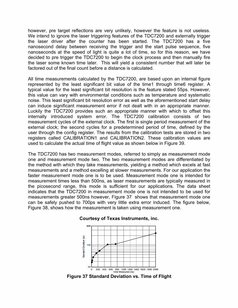
however, pre target reflections are very unlikely, however the feature is not useless. We intend to ignore the laser triggering features of the TDC7200 and externally trigger the laser driver after the counter has been started. The TDC7200 has a five nanosecond delay between receiving the trigger and the start pulse sequence, five nanoseconds at the speed of light is quite a lot of time, so for this reason, we have decided to pre trigger the TDC7200 to begin the clock process and then manually fire the laser some known time later. This will yield a consistent number that will later be factored out of the final count before a distance is calculated. All time measurements calculated by the TDC7200, are based upon an internal figure represented by the least significant bit value of the time1 through time6 register. A typical value for the least significant bit resolution is the feature stated 55ps. However, this value can vary with environmental conditions such as temperature and systematic noise. This least significant bit resolution error as well as the aforementioned start delay can induce significant measurement error if not dealt with in an appropriate manner. Luckily the TDC7200 provides such an appropriate manner with which to offset this internally introduced system error. The TDC7200 calibration consists of two measurement cycles of the external clock. The first is single period measurement of the external clock; the second cycles for a predetermined period of time, defined by the user through the config register. The results from the calibration tests are stored in two registers called CALIBRATION1 and CALIBRATION2. These calibration values are used to calculate the actual time of flight value as shown below in Figure 39. The TDC7200 has two measurement modes, referred to simply as measurement mode one and measurement mode two. The two measurement modes are differentiated by the method with which they take measurements, yielding a method which excels at fast measurements and a method excelling at slower measurements. For our application the faster measurement mode one is to be used. Measurement mode one is intended for measurement times less than 500ns, as laser measurements are typically measured in the picosecond range, this mode is sufficient for our applications. The data sheet indicates that the TDC7200 in measurement mode one is not intended to be used for measurements greater 500ns however, Figure 37 shows that measurement mode one can be safely pushed to 700ps with very little extra error induced. The figure below, Figure 38, shows how the measurement is taken using measurement one.

Courtesy of Texas Instruments, inc.

Figure 37 Standard Deviation vs. Time of Flight

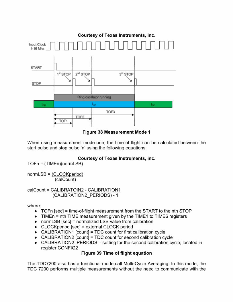
Courtesy of Texas Instruments, inc.

Figure 38 Measurement Mode 1

When using measurement mode one, the time of flight can be calculated between the start pulse and stop pulse ‘n’ using the following equations:

Courtesy of Texas Instruments, inc. TOFn = (TIMEn)(normLSB) normLSB = (CLOCKperiod) (calCount) calCount = CALIBRATOIN2 - CALIBRATION1 (CALIBRATION2_PERIODS) - 1 where: ● TOFn [sec] = time-of-flight measurement from the START to the nth STOP ● TIMEn = nth TIME measurement given by the TIME1 to TIME6 registers ● normLSB [sec] = normalized LSB value from calibration ● CLOCKperiod [sec] = external CLOCK period ● CALIBRATION1 [count] = TDC count for first calibration cycle ● CALIBRATION2 [count] = TDC count for second calibration cycle ● CALIBRATION2_PERIODS = setting for the second calibration cycle; located in

register CONFIG2 Figure 39 Time of flight equation

The TDC7200 also has a functional mode call Multi-Cycle Averaging. In this mode, the TDC 7200 performs multiple measurements without the need to communicate with the

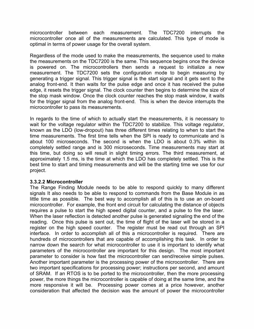
microcontroller between each measurement. The TDC7200 interrupts the microcontroller once all of the measurements are calculated. This type of mode is optimal in terms of power usage for the overall system. Regardless of the mode used to make the measurements, the sequence used to make the measurements on the TDC7200 is the same. This sequence begins once the device is powered on. The microcontrollers then sends a request to initialize a new measurement. The TDC7200 sets the configuration mode to begin measuring by generating a trigger signal. This trigger signal is the start signal and it gets sent to the analog front-end. It then waits for the pulse edge and once it has received the pulse edge, it resets the trigger signal. The clock counter then begins to determine the size of the stop mask window. Once the clock counter reaches the stop mask window, it waits for the trigger signal from the analog front-end. This is when the device interrupts the microcontroller to pass its measurements. In regards to the time of which to actually start the measurements, it is necessary to wait for the voltage regulator within the TDC7200 to stabilize. This voltage regulator, known as the LDO (low-dropout) has three different times relating to when to start the time measurements. The first time tells when the SPI is ready to communicate and is about 100 microseconds. The second is when the LDO is about 0.3% within its completely settled range and is 300 microseconds. Time measurements may start at this time, but doing so will result in slight timing errors. The third measurement, at approximately 1.5 ms, is the time at which the LDO has completely settled. This is the best time to start and timing measurements and will be the starting time we use for our project. 3.3.2.2 Microcontroller The Range Finding Module needs to be able to respond quickly to many different signals It also needs to be able to respond to commands from the Base Module in as little time as possible. The best way to accomplish all of this is to use an on-board microcontroller. For example, the front end circuit for calculating the distance of objects requires a pulse to start the high speed digital counter, and a pulse to fire the laser. When the laser reflection is detected another pulse is generated signaling the end of the reading. Once this pulse is sent out, the time of flight of the laser will be stored in a register on the high speed counter. The register must be read out through an SPI interface. In order to accomplish all of this a microcontroller is required. There are hundreds of microcontrollers that are capable of accomplishing this task. In order to narrow down the search for what microcontroller to use it is important to identify what parameters of the microcontroller are important for this design. The most important parameter to consider is how fast the microcontroller can send/receive simple pulses. Another important parameter is the processing power of the microcontroller. There are two important specifications for processing power; instructions per second, and amount of SRAM. If an RTOS is to be ported to the microcontroller, then the more processing power, the more things the microcontroller is capable of doing at the same time, and the more responsive it will be. Processing power comes at a price however, another consideration that affected the decision was the amount of power the microcontroller

used. The last thing to consider was the actual price of the chip. The following microcontrollers were considered for the final design. 3.3.2.2.1 ARM Cortex m4 ARM Cortex m4 is not a specific microcontroller but an architecture used as the processing core by many microcontroller manufacturers. There are a lot of ARM Cortex m4 processors to choose from. The benefit of these types of microcontrollers is that there are ports for many common firmware libraries which makes software development a lot easier. Another benefit is that most ARM based microcontrollers have very low power modes that the CPU can enter when there is nothing to process. 3.3.2.2.1.1 STM32F407 The STM32F407 is a 32bit microcontroller manufactured by STMicroelectronics. This particular chip has 512 - 1024 KB of FLASH memory for storing the firmware and 192KB of SRAM. It can be clocked at 168MHz which is relatively fast compared to most microcontrollers. Another useful feature is that it has a hardware floating point unit for calculating single precision floating point operations. The internal clock architecture allows for the actual processor to be clocked at many different frequencies, so in order to save power it can be clocked at lower frequencies. When the device is running at 168MHz it draws about X mA. This is quite a lot of power however when the device is waiting for a range reading to complete, or waiting for a command from the Base Module, it can enter low power mode. In low power mode the device draws about YuA. On digikey the 100 pin package for this chip costs $14.24. This microcontroller can definitely accomplish everything that the Range Finding Device needs to do however it is a little more expensive than other microcontrollers. 3.3.2.2.1.2 STM32F427 The STM32F427 is another 32bit microcontroller manufactured by STMicroelectronics. The key differences between this processor and the STM32F407 are in performance and cost. The STM32F427 can be clocked at 180MHz and has 256KB of SRAM. This chip costs $18.60 however if processing power is needed this chip will definitely do the job. 3.3.2.2.2 PSOC5LP The PSOC5LP is a 32bit microcontroller manufactured by Cypress Semiconductors. The PSOC5LP has an ARM Cortex m3 core and can be clocked up to 24MHz. This is much slower than the STM32 chips, however the PSOC5LP is unique from most microcontrollers because its IO system is so general purpose that it can be configured to for implementing digital logic similar to the way a FGPA works. The PSOC5LP is not very cheap compared to some other options available either, it costs between $8.00 and $15.00. 3.3.2.2.3 ATMEGA328p The ATMEGA328p is a 8-bit microcontroller manufactured by ATMEL. The ATMEGA328p can be clocked up to 20MHz however in order to achieve these speeds an external crystal oscillator must be used. Although the ATMEGA328p is the least

powerful of all the microcontrollers considered, what makes this chip a good choice is that there is a large community of developers that have written many libraries for it. This makes developing the firmware much easier. It is also the cheapest of the microcontrollers and costs $4.70. The performance may become a huge issue with this chip however because it is only an 8bit processor and it can only do software floating point operations. This means that a single precision floating point operation could take hundreds of instructions to finish and take on the order of a tenth of a millisecond to complete. If a lot of complex math is needed than this chip will not be able to keep up. The microcontroller that was selected for the range finding module was the STM32F407. The reason this chip was selected was because it is guaranteed to be fast enough to accomplish the tasks required. The price did not have very much weight in the decision because this design is for a prototype system. When this project moves into the production stage, this microcontroller may be replaced with a cheaper one. 3.3.3 Optics There were many different options that were available for the optical front-end design. Initially the optics was designed to be custom for this particular design. When the design was finished the total price for all of the optical elements came out to be very expensive. It was decided that instead of trying to put together a custom optical front end, it would be cheaper to buy one that has already been designed. The reason it is cheaper to buy the optical systems already assembled are because they are in a more mature stage in their project life cycle, and are optimized for price and performance. The optics lens we chose to use to perform projecting the laser, receiving the laser and collimating the incoming laser are Plano-convex acrylic lens that will each be connected to their own Polyacrylonitrile Butadiene Styrene (ABS) with 30% glass fibre alignment tubes and lens tubes. The optics will also include circuitry to determine the timing of when the laser has been fired and when the laser reaches the receiving lens to signify the time-to-digital converter to stop timing.

This part of the design phase relied heavily on the project researched and documented in section 2.1.3. We decided to use the same amplifier circuit, photodiode and laser driver that was used on the OSLRF-01. However, in order to control our timing signals, we chose to use the TDC7200 rather than the timebase expander used for that project. For more information about how timing the signals using the TDC7200, refer to section 3.3.2.1. 3.3.3.1 Transmitter The optics of a laser rangefinder consists of a transmitter section and a receiver section. For more information about the functions of the optics, please refer to section 2.4.2. The transmitter section is responsible for providing a pulsed laser source, a laser driver circuit, and a trigger circuit. The next few sections describe these components within the transmitting end of the laser rangefinder.

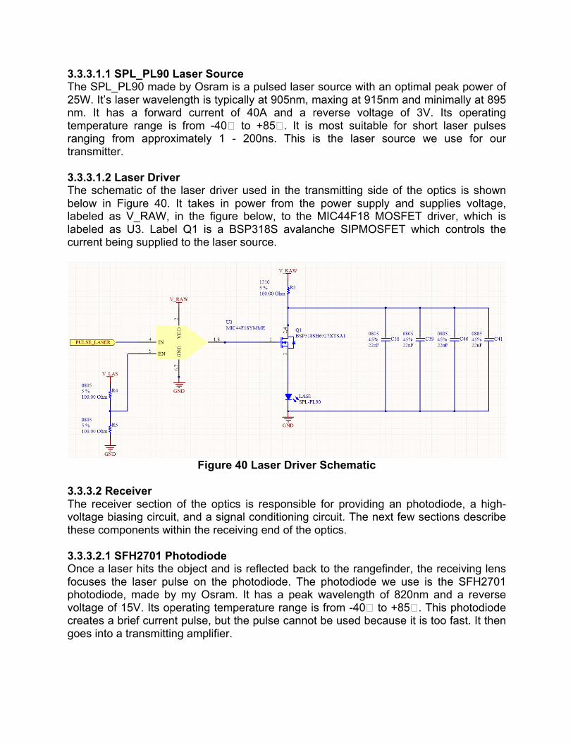
3.3.3.1.1 SPL_PL90 Laser Source The SPL_PL90 made by Osram is a pulsed laser source with an optimal peak power of 25W. It’s laser wavelength is typically at 905nm, maxing at 915nm and minimally at 895 nm. It has a forward current of 40A and a reverse voltage of 3V. Its operating temperature range is from -40� to +85�. It is most suitable for short laser pulses ranging from approximately 1 - 200ns. This is the laser source we use for our transmitter. 3.3.3.1.2 Laser Driver The schematic of the laser driver used in the transmitting side of the optics is shown below in Figure 40. It takes in power from the power supply and supplies voltage, labeled as V_RAW, in the figure below, to the MIC44F18 MOSFET driver, which is labeled as U3. Label Q1 is a BSP318S avalanche SIPMOSFET which controls the current being supplied to the laser source.

Figure 40 Laser Driver Schematic

3.3.3.2 Receiver The receiver section of the optics is responsible for providing an photodiode, a high-voltage biasing circuit, and a signal conditioning circuit. The next few sections describe these components within the receiving end of the optics. 3.3.3.2.1 SFH2701 Photodiode Once a laser hits the object and is reflected back to the rangefinder, the receiving lens focuses the laser pulse on the photodiode. The photodiode we use is the SFH2701 photodiode, made by my Osram. It has a peak wavelength of 820nm and a reverse voltage of 15V. Its operating temperature range is from -40� to +85�. This photodiode creates a brief current pulse, but the pulse cannot be used because it is too fast. It then goes into a transmitting amplifier.

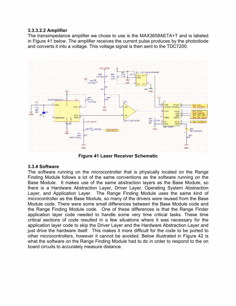
3.3.3.2.2 Amplifier The transimpedance amplifier we chose to use is the MAX3658AETA+T and is labeled in Figure 41 below. The amplifier receives the current pulse produces by the photodiode and converts it into a voltage. This voltage signal is then sent to the TDC7200.

Figure 41 Laser Receiver Schematic

3.3.4 Software The software running on the microcontroller that is physically located on the Range Finding Module follows a lot of the same conventions as the software running on the Base Module. It makes use of the same abstraction layers as the Base Module, so there is a Hardware Abstraction Layer, Driver Layer, Operating System Abstraction Layer, and Application Layer. The Range Finding Module uses the same kind of microcontroller as the Base Module, so many of the drivers were reused from the Base Module code. There were some small differences between the Base Module code and the Range Finding Module code. One of these differences is that the Range Finder application layer code needed to handle some very time critical tasks. These time critical sections of code resulted in a few situations where it was necessary for the application layer code to skip the Driver Layer and the Hardware Abstraction Layer and just drive the hardware itself. This makes it more difficult for the code to be ported to other microcontrollers, however it cannot be avoided. Below illustrated in Figure 42 is what the software on the Range Finding Module had to do in order to respond to the on board circuits to accurately measure distance.

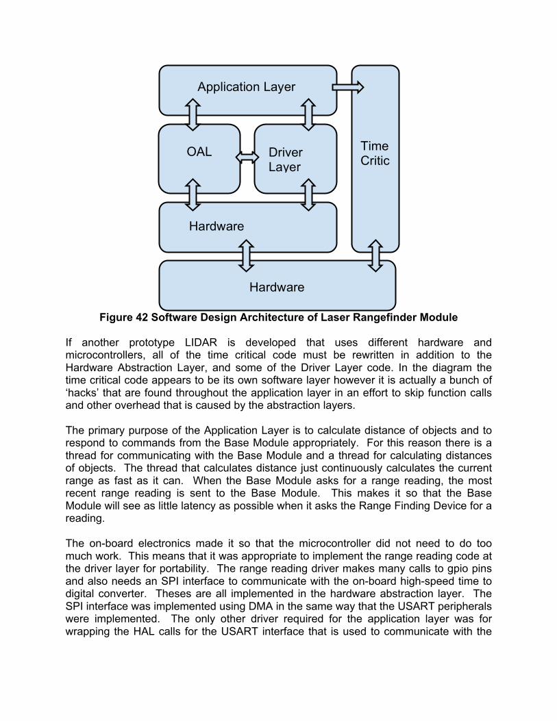
Figure 42 Software Design Architecture of Laser Rangefinder Module

If another prototype LIDAR is developed that uses different hardware and microcontrollers, all of the time critical code must be rewritten in addition to the Hardware Abstraction Layer, and some of the Driver Layer code. In the diagram the time critical code appears to be its own software layer however it is actually a bunch of ‘hacks’ that are found throughout the application layer in an effort to skip function calls and other overhead that is caused by the abstraction layers. The primary purpose of the Application Layer is to calculate distance of objects and to respond to commands from the Base Module appropriately. For this reason there is a thread for communicating with the Base Module and a thread for calculating distances of objects. The thread that calculates distance just continuously calculates the current range as fast as it can. When the Base Module asks for a range reading, the most recent range reading is sent to the Base Module. This makes it so that the Base Module will see as little latency as possible when it asks the Range Finding Device for a reading. The on-board electronics made it so that the microcontroller did not need to do too much work. This means that it was appropriate to implement the range reading code at the driver layer for portability. The range reading driver makes many calls to gpio pins and also needs an SPI interface to communicate with the on-board high-speed time to digital converter. Theses are all implemented in the hardware abstraction layer. The SPI interface was implemented using DMA in the same way that the USART peripherals were implemented. The only other driver required for the application layer was for wrapping the HAL calls for the USART interface that is used to communicate with the

Application Layer

OAL Driver Layer

Hardware Abstraction Layer

Time Critical

Hardware

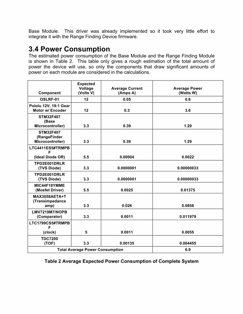
Base Module. This driver was already implemented so it took very little effort to integrate it with the Range Finding Device firmware. 3.4 Power Consumption The estimated power consumption of the Base Module and the Range Finding Module is shown in Table 2. This table only gives a rough estimation of the total amount of power the device will use, so only the components that draw significant amounts of power on each module are considered in the calculations.

Component

Expected Voltage (Volts V)

Average Current (Amps A)

Average Power (Watts W)

OSLRF-01 12 0.05 0.6 Pololu 12V, 19:1 Gear

Motor w/ Encoder 12 0.3 3.6 STM32F407

(Base Microcontroller) 3.3 0.39 1.29

STM32F407 (RangeFinder

Microcontroller) 3.3 0.39 1.29 LTC4411ES5#TRMPB

F (Ideal Diode OR) 5.5 0.00004 0.0022 TPD2E001DRLR

(TVS Diode) 3.3 0.0000001 0.00000033 TPD2E001DRLR

(TVS Diode) 3.3 0.0000001 0.00000033 MIC44F18YMME (Mosfet Driver) 5.5 0.0025 0.01375

MAX3658AETA+T (Transimpedance

amp) 3.3 0.026 0.0858 LMV7219M7/NOPB

(Comparator) 3.3 0.0011 0.011979 LTC1799CS5#TRMPB

F (clock) 5 0.0011 0.0055

TDC7200 (TOF) 3.3 0.00135 0.004455

Total Average Power Consumption 6.9

Table 2 Average Expected Power Consumption of Complete System

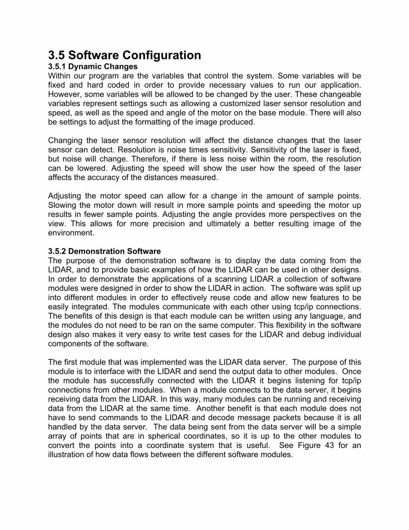
3.5 Software Configuration 3.5.1 Dynamic Changes Within our program are the variables that control the system. Some variables will be fixed and hard coded in order to provide necessary values to run our application. However, some variables will be allowed to be changed by the user. These changeable variables represent settings such as allowing a customized laser sensor resolution and speed, as well as the speed and angle of the motor on the base module. There will also be settings to adjust the formatting of the image produced. Changing the laser sensor resolution will affect the distance changes that the laser sensor can detect. Resolution is noise times sensitivity. Sensitivity of the laser is fixed, but noise will change. Therefore, if there is less noise within the room, the resolution can be lowered. Adjusting the speed will show the user how the speed of the laser affects the accuracy of the distances measured. Adjusting the motor speed can allow for a change in the amount of sample points. Slowing the motor down will result in more sample points and speeding the motor up results in fewer sample points. Adjusting the angle provides more perspectives on the view. This allows for more precision and ultimately a better resulting image of the environment. 3.5.2 Demonstration Software The purpose of the demonstration software is to display the data coming from the LIDAR, and to provide basic examples of how the LIDAR can be used in other designs. In order to demonstrate the applications of a scanning LIDAR a collection of software modules were designed in order to show the LIDAR in action. The software was split up into different modules in order to effectively reuse code and allow new features to be easily integrated. The modules communicate with each other using tcp/ip connections. The benefits of this design is that each module can be written using any language, and the modules do not need to be ran on the same computer. This flexibility in the software design also makes it very easy to write test cases for the LIDAR and debug individual components of the software. The first module that was implemented was the LIDAR data server. The purpose of this module is to interface with the LIDAR and send the output data to other modules. Once the module has successfully connected with the LIDAR it begins listening for tcp/ip connections from other modules. When a module connects to the data server, it begins receiving data from the LIDAR. In this way, many modules can be running and receiving data from the LIDAR at the same time. Another benefit is that each module does not have to send commands to the LIDAR and decode message packets because it is all handled by the data server. The data being sent from the data server will be a simple array of points that are in spherical coordinates, so it is up to the other modules to convert the points into a coordinate system that is useful. See Figure 43 for an illustration of how data flows between the different software modules.

Figure 43 Demonstration Software Data Flow

The tcp/ip stack has buffer size limitations, so if there is a lot of data it is not guaranteed that all of the data will be sent in the same packet. For this reason it was decided that there needed to be a framing layer for packaging multiple tcp packets into one data packet. For consistency SLIP was used for this purpose. Although it may be considered redundant to add more overhead, the SLIP layer prevents errors from occurring during data transmission. For example, if a packet gets split in half then the client may not be able to properly decode the data. 3.5.2.1 Native Data Visualizer The next module that was implemented is a data visualizer. This module was designed to run natively on linux, mac, and windows operating systems. The purpose of this module is to simply receive the data from the data server then plot the data points on a 3d graph in real-time. Although the data is real-time, each data point received from the LIDAR can be configured to persist for a few seconds allowing the entire scene to be visualized in 3d. The benefit of allowing the points to persist for a period of time is that it allows more than just one LIDAR scan to be visualized, so instead of seeing just one line, the user will see a cloud of points corresponding to different objects in the scene. Being able to visualize the data from the LIDAR not only serves as a demonstration, but

it is also a good tool for testing the system to make sure that it meets all of its specifications. In order to be cross-platform the language that was chosen for this application was java. Although java does not technically compile down to native machine language, the application is still considered native because it only displays incoming data locally on the machine that it is run on. Java does not have any 3d graphics built in so a library called LWJGL was included in the project. LWJGL is a library that wraps opengl functions so that they can be called through the Java Native Interface (JNI). Even though the code for the native data visualizer is written in java it still needs to be packaged for different operating systems. The reason the code has to be packaged differently is because LWJGL makes native function calls. This means that there is native binary code that has to be linked to the java application. Currently the supported operating systems that this application has been packaged for are linux, mac, and windows. In the future the application could be packaged for any operating system that is supported by LWJGL. 3.5.2.2 Web Client The web client module is designed to be a data visualizer that can be viewed from an internet browser. This module provides a way that any device can be used to view the data coming from the LIDAR. The native visualizer is more convenient for systems that support it. The web client provides a way for devices that the native client is not packaged for. The client module has two components; the server and the client. The web server component is not the same thing as the data server described in section 4.4.1. This server is designed to connect to the data server get data from it, and serve it to a webservice. The server is written in javascript using a javascript runtime called nodejs. The benefit of nodejs is that it allows javascript code to be ran without a web browser and it has a bunch of built in libraries for designing server code. The nodejs server connects to the data server using tcp/ip, and serves the web page to a browser. In order to run the server the user must make sure that they have nodejs installed on their computer. Nodejs is supported by linux, mac, and windows so the server is very versatile. The client is written in html and javascript because it is designed to be loaded in a browser. The client using a html5 canvas to create a webgl context. Once the webgl context is initialized, the client begins receiving data from the nodejs server, and plotting the data points in 3d. In order to run the client in a browser it is important to make sure that webgl is supported and enabled in the browser settings. Once the nodejs server is running the user can open their browser and connect to the server by typing in the server ip and port. Any computer that is connected to the same subnet as the nodejs server can load the webpage and view the data coming from the LIDAR. The benefit of being able to view the data in a browser is that now smart

phones can access the data coming from the LIDAR, and with the correct port forwarding, the LIDAR data can even be viewed remotely. 3.5.2.3 Android App The android app module works the same way as the native app. It would have been too difficult to try and port the native app to the android framework. Instead of porting the native app to android, a new app was written in order to view data on android. Even though many android devices can view the data in their browser, it was decided that having an app dedicated to viewing data on an android phone would be more convenient, and run faster. The android app was written in java and uses LWJGL to access the graphics hardware. A lot of the code used in the native app was reused in the android app. For example, because websockets are standardized in java so all of the code that the native app used to connect to the data server was reused in the the android app. 3.6 System Schematics 3.6.1 Base Module The schematics that follow take on a hierarchical structure, and are listed from highest level to lowest level. The highest level schematic shows how all of the other schematics connect to each other and to the outside world. The green elements represent other schematics, and the yellow elements represent different parts that are on the board. The schematics were designed this way in order to make them more readable, and to make it easier to catch errors.

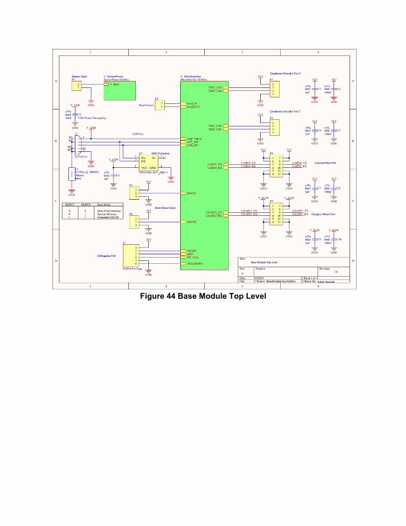
Figure 44 Base Module Top Level

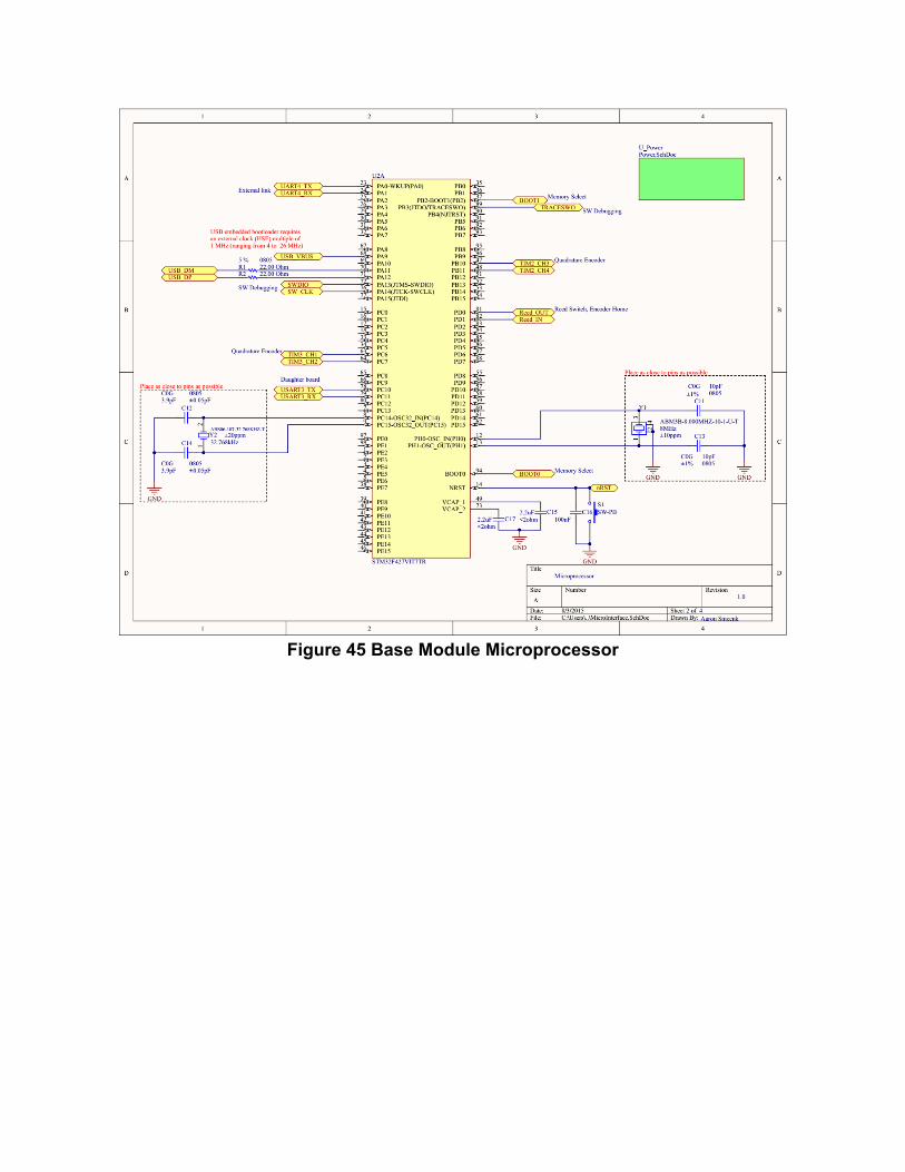
Figure 45 Base Module Microprocessor

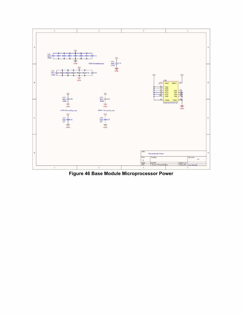
Figure 46 Base Module Microprocessor Power

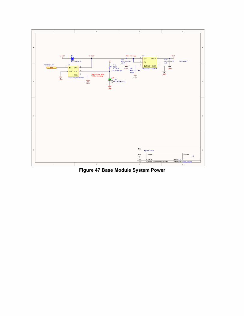
Figure 47 Base Module System Power

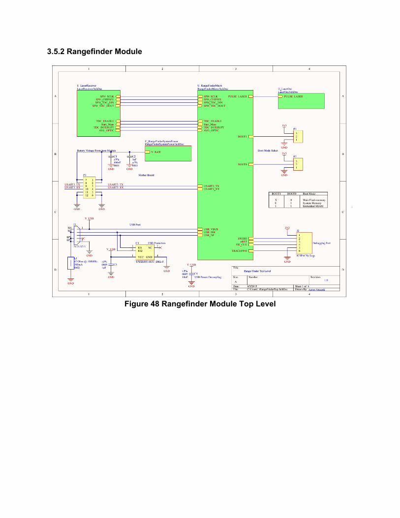
3.5.2 Rangefinder Module

Figure 48 Rangefinder Module Top Level

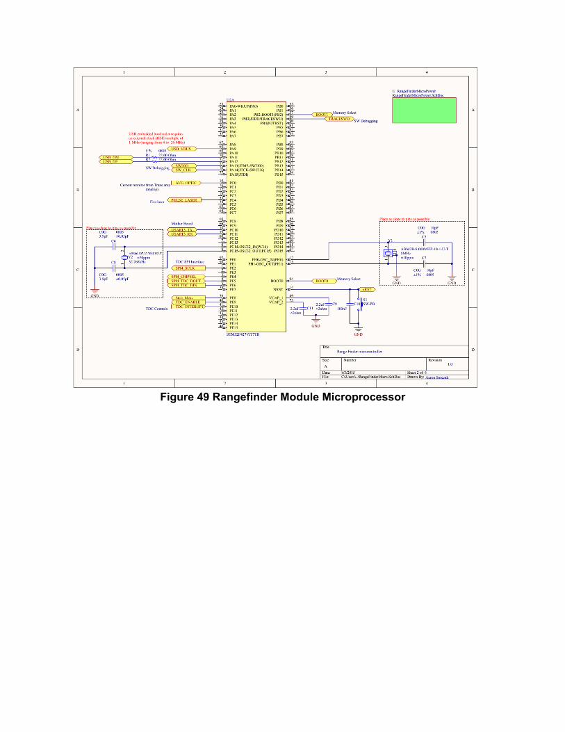
Figure 49 Rangefinder Module Microprocessor

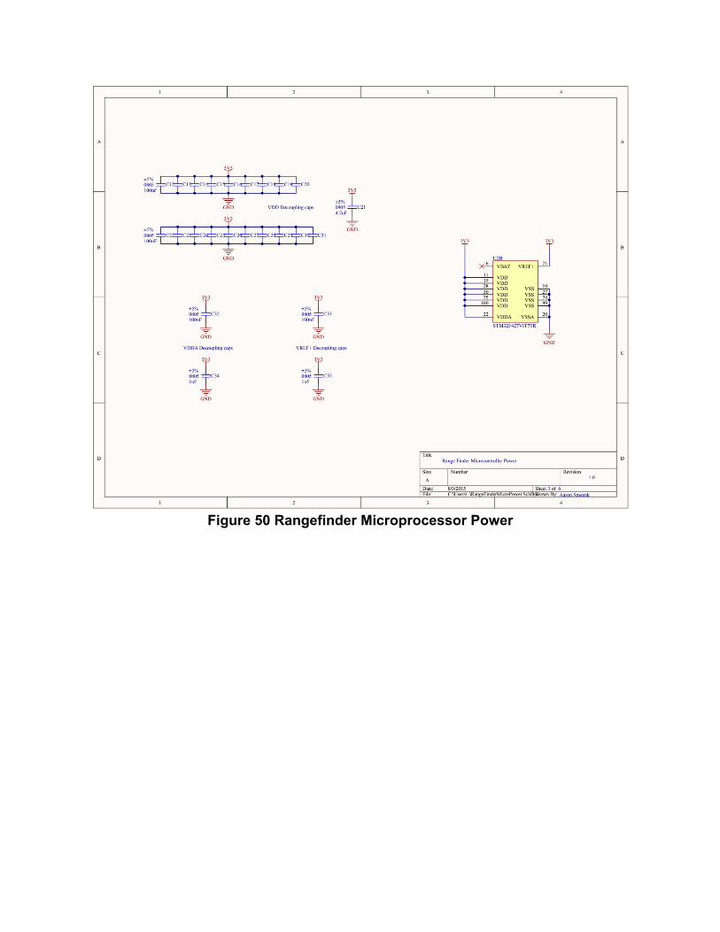
Figure 50 Rangefinder Microprocessor Power

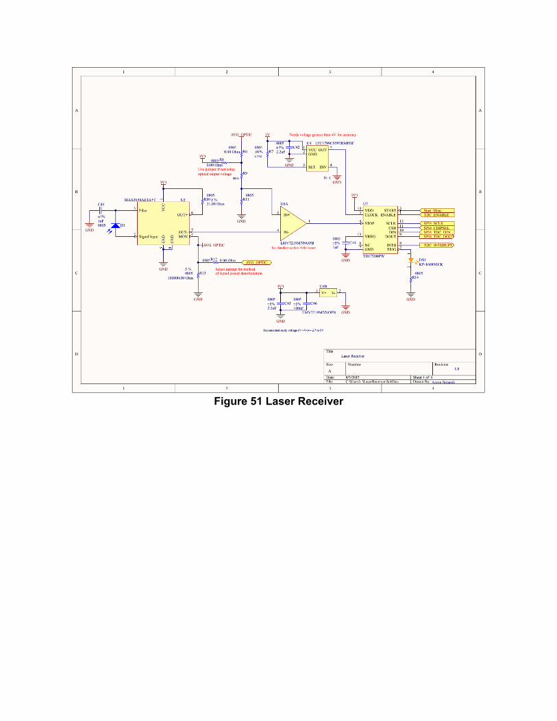
Figure 51 Laser Receiver

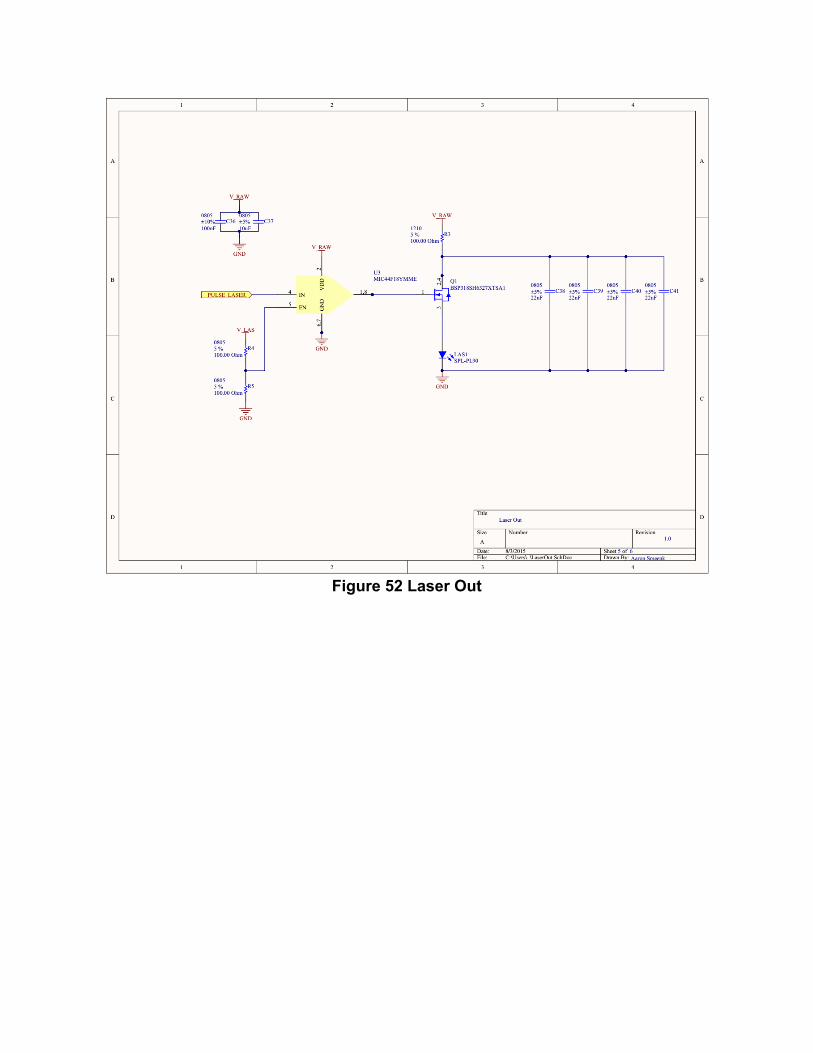
Figure 52 Laser Out

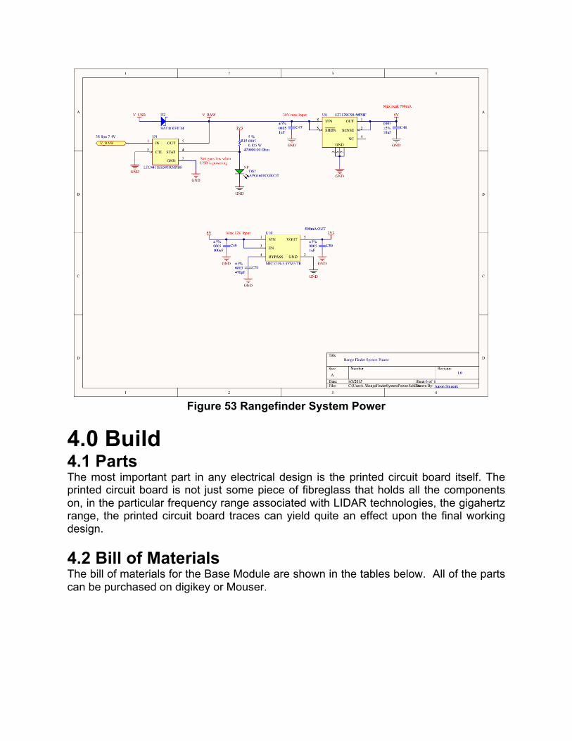
Figure 53 Rangefinder System Power

4.0 Build

4.1 Parts The most important part in any electrical design is the printed circuit board itself. The printed circuit board is not just some piece of fibreglass that holds all the components on, in the particular frequency range associated with LIDAR technologies, the gigahertz range, the printed circuit board traces can yield quite an effect upon the final working design. 4.2 Bill of Materials The bill of materials for the Base Module are shown in the tables below. All of the parts can be purchased on digikey or Mouser.

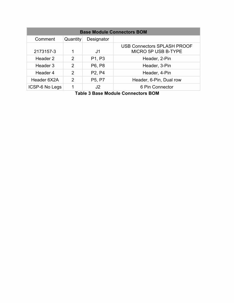
Base Module Connectors BOM Comment Quantity Designator

2173157-3 1 J1 USB Connectors SPLASH PROOF

MICRO 5P USB B-TYPE Header 2 2 P1, P3 Header, 2-Pin Header 3 2 P6, P8 Header, 3-Pin Header 4 2 P2, P4 Header, 4-Pin

Header 6X2A 2 P5, P7 Header, 6-Pin, Dual row ICSP-6 No Legs 1 J2 6 Pin Connector

Table 3 Base Module Connectors BOM

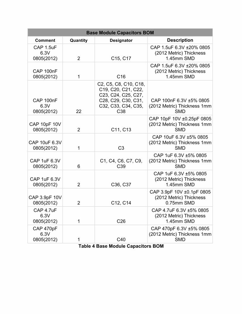
Base Module Capacitors BOM Comment Quantity Designator Description

CAP 1.5uF 6.3V

0805(2012) 2 C15, C17

CAP 1.5uF 6.3V ±20% 0805 (2012 Metric) Thickness

1.45mm SMD

CAP 100nF 0805(2012) 1 C16

CAP 1.5uF 6.3V ±20% 0805 (2012 Metric) Thickness

1.45mm SMD

CAP 100nF 6.3V

0805(2012) 22

C2, C5, C8, C10, C18, C19, C20, C21, C22, C23, C24, C25, C27, C28, C29, C30, C31, C32, C33, C34, C35,

C38

CAP 100nF 6.3V ±5% 0805 (2012 Metric) Thickness 1mm

SMD

CAP 10pF 10V 0805(2012) 2 C11, C13

CAP 10pF 10V ±0.25pF 0805 (2012 Metric) Thickness 1mm

SMD

CAP 10uF 6.3V 0805(2012) 1 C3

CAP 10uF 6.3V ±5% 0805 (2012 Metric) Thickness 1mm

SMD

CAP 1uF 6.3V 0805(2012) 6

C1, C4, C6, C7, C9, C39

CAP 1uF 6.3V ±5% 0805 (2012 Metric) Thickness 1mm

SMD

CAP 1uF 6.3V 0805(2012) 2 C36, C37

CAP 1uF 6.3V ±5% 0805 (2012 Metric) Thickness

1.45mm SMD

CAP 3.9pF 10V 0805(2012) 2 C12, C14

CAP 3.9pF 10V ±0.1pF 0805 (2012 Metric) Thickness

0.75mm SMD CAP 4.7uF

6.3V 0805(2012) 1 C26

CAP 4.7uF 6.3V ±5% 0805 (2012 Metric) Thickness

1.45mm SMD CAP 470pF

6.3V 0805(2012) 1 C40

CAP 470pF 6.3V ±5% 0805 (2012 Metric) Thickness 1mm

SMD Table 4 Base Module Capacitors BOM

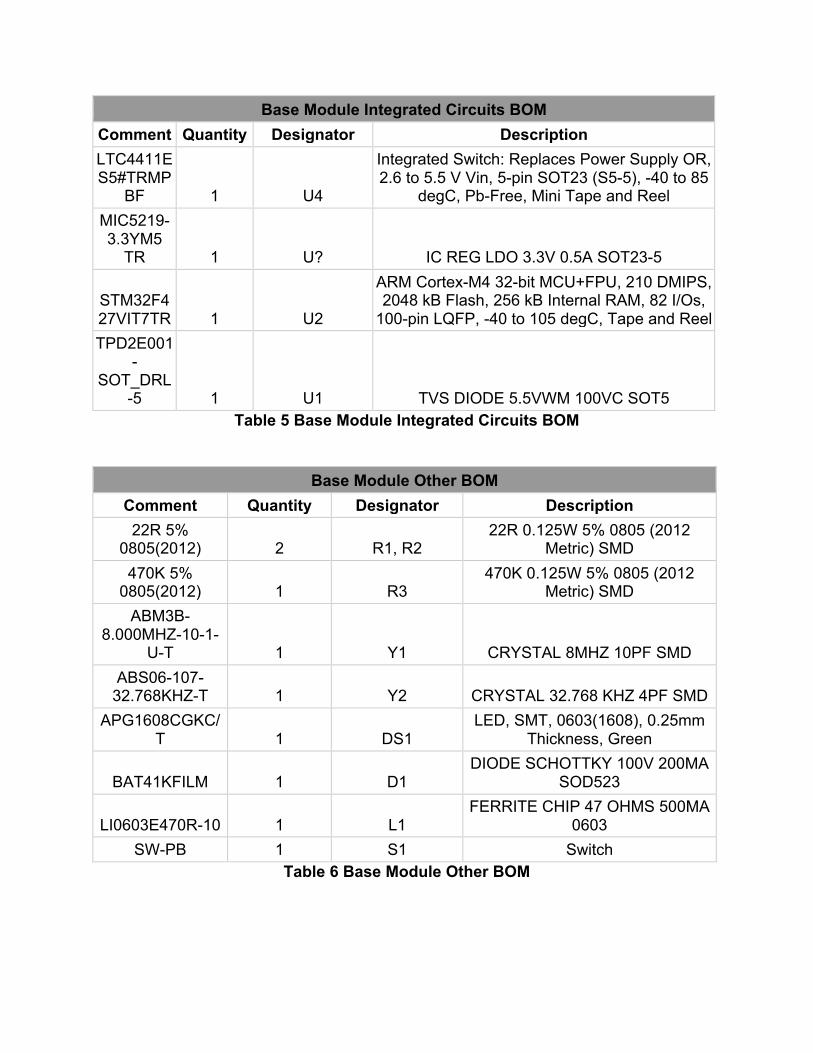
Base Module Integrated Circuits BOM Comment Quantity Designator Description LTC4411ES5#TRMP

BF 1 U4

Integrated Switch: Replaces Power Supply OR, 2.6 to 5.5 V Vin, 5-pin SOT23 (S5-5), -40 to 85

degC, Pb-Free, Mini Tape and Reel MIC5219-3.3YM5

TR 1 U? IC REG LDO 3.3V 0.5A SOT23-5

STM32F427VIT7TR 1 U2

ARM Cortex-M4 32-bit MCU+FPU, 210 DMIPS, 2048 kB Flash, 256 kB Internal RAM, 82 I/Os,

100-pin LQFP, -40 to 105 degC, Tape and Reel TPD2E001

-SOT_DRL

-5 1 U1 TVS DIODE 5.5VWM 100VC SOT5 Table 5 Base Module Integrated Circuits BOM

Base Module Other BOM Comment Quantity Designator Description 22R 5%

0805(2012) 2 R1, R2 22R 0.125W 5% 0805 (2012

Metric) SMD 470K 5%

0805(2012) 1 R3 470K 0.125W 5% 0805 (2012

Metric) SMD ABM3B-

8.000MHZ-10-1-U-T 1 Y1 CRYSTAL 8MHZ 10PF SMD

ABS06-107-32.768KHZ-T 1 Y2 CRYSTAL 32.768 KHZ 4PF SMD

APG1608CGKC/T 1 DS1

LED, SMT, 0603(1608), 0.25mm Thickness, Green

BAT41KFILM 1 D1 DIODE SCHOTTKY 100V 200MA

SOD523

LI0603E470R-10 1 L1 FERRITE CHIP 47 OHMS 500MA

0603 SW-PB 1 S1 Switch

Table 6 Base Module Other BOM

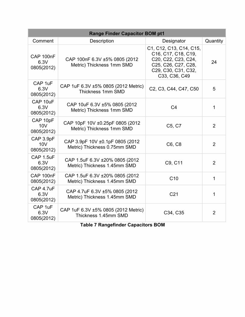
Range Finder Capacitor BOM pt1 Comment Description Designator Quantity

CAP 100nF 6.3V

0805(2012)

CAP 100nF 6.3V ±5% 0805 (2012 Metric) Thickness 1mm SMD

C1, C12, C13, C14, C15, C16, C17, C18, C19, C20, C22, C23, C24, C25, C26, C27, C28, C29, C30, C31, C32,

C33, C36, C49

24

CAP 1uF 6.3V

0805(2012)

CAP 1uF 6.3V ±5% 0805 (2012 Metric) Thickness 1mm SMD C2, C3, C44, C47, C50 5

CAP 10uF 6.3V

0805(2012)

CAP 10uF 6.3V ±5% 0805 (2012 Metric) Thickness 1mm SMD C4 1

CAP 10pF 10V

0805(2012)

CAP 10pF 10V ±0.25pF 0805 (2012 Metric) Thickness 1mm SMD C5, C7 2

CAP 3.9pF 10V

0805(2012)

CAP 3.9pF 10V ±0.1pF 0805 (2012 Metric) Thickness 0.75mm SMD C6, C8 2

CAP 1.5uF 6.3V

0805(2012)

CAP 1.5uF 6.3V ±20% 0805 (2012 Metric) Thickness 1.45mm SMD C9, C11 2

CAP 100nF 0805(2012)

CAP 1.5uF 6.3V ±20% 0805 (2012 Metric) Thickness 1.45mm SMD C10 1

CAP 4.7uF 6.3V

0805(2012)

CAP 4.7uF 6.3V ±5% 0805 (2012 Metric) Thickness 1.45mm SMD C21 1

CAP 1uF 6.3V

0805(2012)

CAP 1uF 6.3V ±5% 0805 (2012 Metric) Thickness 1.45mm SMD C34, C35 2

Table 7 Rangefinder Capacitors BOM

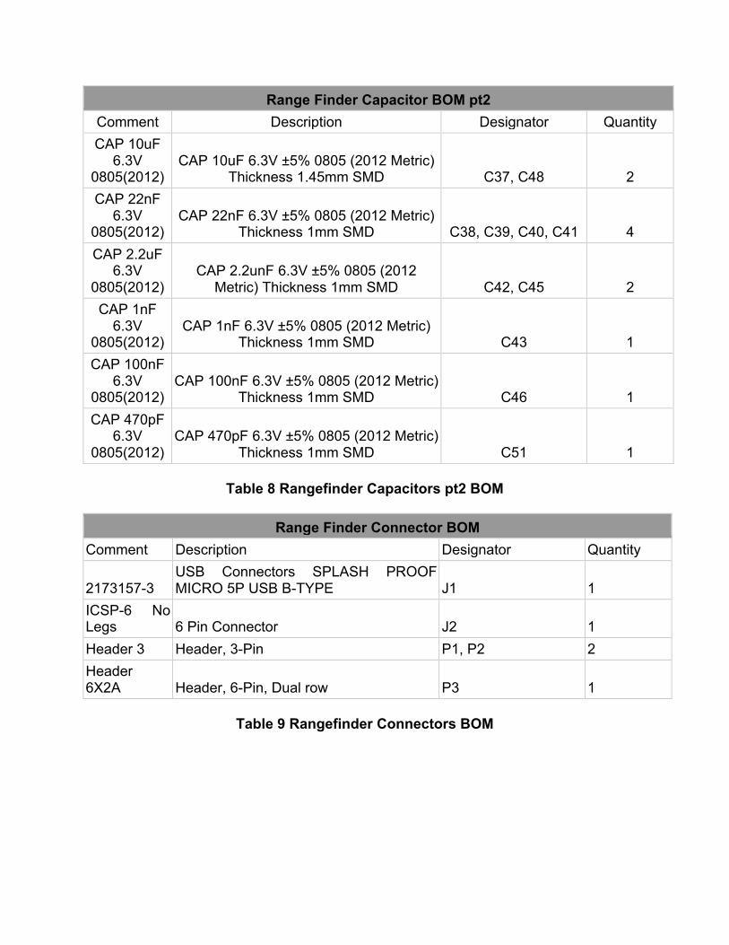
Range Finder Capacitor BOM pt2 Comment Description Designator Quantity CAP 10uF

6.3V 0805(2012)

CAP 10uF 6.3V ±5% 0805 (2012 Metric) Thickness 1.45mm SMD C37, C48 2

CAP 22nF 6.3V

0805(2012) CAP 22nF 6.3V ±5% 0805 (2012 Metric)

Thickness 1mm SMD C38, C39, C40, C41 4 CAP 2.2uF

6.3V 0805(2012)

CAP 2.2unF 6.3V ±5% 0805 (2012 Metric) Thickness 1mm SMD C42, C45 2

CAP 1nF 6.3V

0805(2012) CAP 1nF 6.3V ±5% 0805 (2012 Metric)

Thickness 1mm SMD C43 1 CAP 100nF

6.3V 0805(2012)

CAP 100nF 6.3V ±5% 0805 (2012 Metric) Thickness 1mm SMD C46 1

CAP 470pF 6.3V

0805(2012) CAP 470pF 6.3V ±5% 0805 (2012 Metric)

Thickness 1mm SMD C51 1

Table 8 Rangefinder Capacitors pt2 BOM

Range Finder Connector BOM Comment Description Designator Quantity

2173157-3 USB Connectors SPLASH PROOF MICRO 5P USB B-TYPE J1 1

ICSP-6 No Legs 6 Pin Connector J2 1 Header 3 Header, 3-Pin P1, P2 2 Header 6X2A Header, 6-Pin, Dual row P3 1

Table 9 Rangefinder Connectors BOM

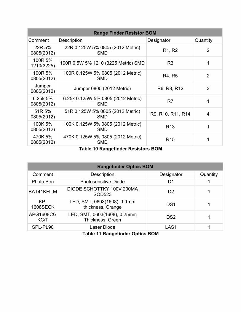
Range Finder Resistor BOM Comment Description Designator Quantity

22R 5% 0805(2012)

22R 0.125W 5% 0805 (2012 Metric) SMD R1, R2 2

100R 5% 1210(3225) 100R 0.5W 5% 1210 (3225 Metric) SMD R3 1

100R 5% 0805(2012)

100R 0.125W 5% 0805 (2012 Metric) SMD R4, R5 2

Jumper 0805(2012) Jumper 0805 (2012 Metric) R6, R8, R12 3

6.25k 5% 0805(2012)

6.25k 0.125W 5% 0805 (2012 Metric) SMD R7 1

51R 5% 0805(2012)

51R 0.125W 5% 0805 (2012 Metric) SMD R9, R10, R11, R14 4

100K 5% 0805(2012)

100K 0.125W 5% 0805 (2012 Metric) SMD R13 1

470K 5% 0805(2012)

470K 0.125W 5% 0805 (2012 Metric) SMD R15 1

Table 10 Rangefinder Resistors BOM

Rangefinder Optics BOM Comment Description Designator Quantity Photo Sen Photosensitive Diode D1 1

BAT41KFILM DIODE SCHOTTKY 100V 200MA SOD523 D2 1

KP-1608SECK

LED, SMT, 0603(1608), 1.1mm thickness, Orange DS1 1

APG1608CGKC/T

LED, SMT, 0603(1608), 0.25mm Thickness, Green DS2 1

SPL-PL90 Laser Diode LAS1 1 Table 11 Rangefinder Optics BOM

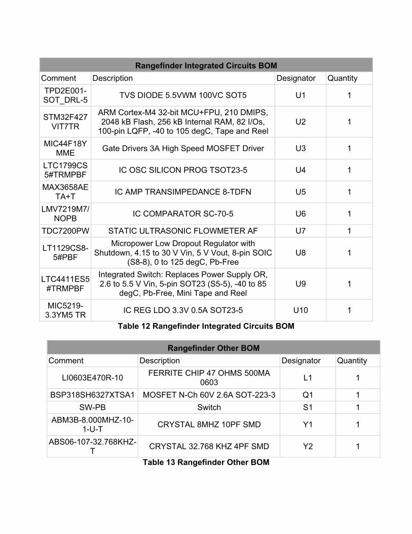
Rangefinder Integrated Circuits BOM

Comment Description Designator Quantity TPD2E001-SOT_DRL-5 TVS DIODE 5.5VWM 100VC SOT5 U1 1

STM32F427VIT7TR

ARM Cortex-M4 32-bit MCU+FPU, 210 DMIPS, 2048 kB Flash, 256 kB Internal RAM, 82 I/Os,

100-pin LQFP, -40 to 105 degC, Tape and Reel U2 1

MIC44F18YMME Gate Drivers 3A High Speed MOSFET Driver U3 1

LTC1799CS5#TRMPBF IC OSC SILICON PROG TSOT23-5 U4 1

MAX3658AETA+T IC AMP TRANSIMPEDANCE 8-TDFN U5 1

LMV7219M7/NOPB IC COMPARATOR SC-70-5 U6 1

TDC7200PW STATIC ULTRASONIC FLOWMETER AF U7 1

LT1129CS8-5#PBF

Micropower Low Dropout Regulator with Shutdown, 4.15 to 30 V Vin, 5 V Vout, 8-pin SOIC

(S8-8), 0 to 125 degC, Pb-Free U8 1

LTC4411ES5#TRMPBF

Integrated Switch: Replaces Power Supply OR, 2.6 to 5.5 V Vin, 5-pin SOT23 (S5-5), -40 to 85

degC, Pb-Free, Mini Tape and Reel U9 1

MIC5219-3.3YM5 TR IC REG LDO 3.3V 0.5A SOT23-5 U10 1

Table 12 Rangefinder Integrated Circuits BOM

Rangefinder Other BOM Comment Description Designator Quantity

LI0603E470R-10 FERRITE CHIP 47 OHMS 500MA 0603 L1 1

BSP318SH6327XTSA1 MOSFET N-Ch 60V 2.6A SOT-223-3 Q1 1 SW-PB Switch S1 1

ABM3B-8.000MHZ-10-1-U-T CRYSTAL 8MHZ 10PF SMD Y1 1

ABS06-107-32.768KHZ-T CRYSTAL 32.768 KHZ 4PF SMD Y2 1

Table 13 Rangefinder Other BOM

5.0 Test

5.1 Instructables RangeFinder The instructables project was included as more or less a proof of concept project. Its purpose was to get a first look at LIDAR and begin to generate data to be used for post processing. The biggest problem with the Instructables LIDAR is that it uses an IR LED within the range finding device, this LED works fine in typical range finding applications as a single point range. In lidar however this single point is rotated about at least one axis. An LED has a very wide beam width that gets larger the further out it travels, just like anything else, but by starting with an exceptionally large beam with we start to have problems once it begins taking multiple samples at a fast rate while rotating. The first test to be performed on the instructables project is to test its beam width at various distances from the LED. The following Table 14 will be populated once the test is formally conducted. The test conducted will be performed by mounting the range finding device to a solid surface and drawing a center-line from the center of the LED extending some distance out. Within the table the left edge and right edge will be measured in millimeters from the centerline of the LED to the place where a detection of a pencil no longer occurs. The initial test will consist of only five data points to establish a general beam width and more points can be added accordingly as needed for greater resolution within a particular region. The second test to be performed on the Instructables project is signal strength return for both white and black surfaces. The purpose of this test is to determine if the maximum range for measurement is due to the beam width or the signal strength and specifically what the maximum range the IR range finder can physically measure. In this test depicted in Table 15 below will be to mount the IR range finder on a solid surface and incrementally move both a black sheet and a white sheet of construction paper out along the centerline of the LED until the device ceases to generate an accurate measurement. The final test to be run is to test if oversampling can effectively average out the effect of the large beam width. The test would be run by moving the servo motor at a fixed rate that is slow enough to allow some set number of samples for a given position on the servomotor. If we were to average together 100 readings per servo position to see the effect on the point cloud output from the system. Once the oversampled point cloud was generated we would compare with the original sampled point cloud. Obvously this test is not very objective, the idea is more to test the theory of oversampling, a technique the group intends to put to use in the final design of the LIDAR unit. 5.2 Base Module 5.2.1 Motor Whenever considering the use of a motor within a system, the motor is chosen based on the specifications granted. The first task that needs to be done is testing that these specifications are accurate. In addition to testing the accuracy of the specifications of the motor, communication between the motor and the microcontroller connected must

be tested in order to confirm the necessary communication requirements between the two devices for this system. Receiving the rotation angle from the encoder is fundamental for acquiring the necessary information to calculate position within the point cloud. This will be one of the first tests done to the motor and encoder. The next test will be to toggle the speed of rotation of the motor. This will allow us to determine the optimal speed at which to scan an environment. We will also test the motor functions to guarantee that the motor works to the standards defined within the data sheet for the RB-Pol-123. These standards include full operation for the motor at 12V which provides 500 revolutions per minute, and 300mA free-run. The encoder gives a 64 counts per revolution of the motor shaft. 5.2.2 Microcontroller The base module microcontroller will be responsible for communication between the external device and the rangefinder module. It will also need to be able to communicate with the motor and encoder to control motor speed and receive the information about the angular rotation of the encoder. Testing these functions will begin with the communication between this microcontroller and the external device, which in this case will be a computer. We will use software tests to demonstrate that the UART communication is properly producing correct data out by harding coding specific values into registers on the microcontroller. Once the values retrieved are correct we will begin to test the USB port for communication as another option. We will perform this test in the same manner as testing the UART. Once we have confirmed that the microcontroller properly communicates with the external device, we will begin testing the communication between this microcontroller and the microcontroller used for the rangefinder module. These two microcontroller will communicate through UART. They will both need to send and receive information from each other. After confirming that the microcontroller used by the rangefinder module works properly, we will connect the two microcontrollers through the UART ports and pass information between the two. We will first connect the base module microcontroller to the computer to load data that will be passed to the rangefinder microcontroller. Then the rangefinder microcontroller will be connected to another computer and the data sent to it from the base module microcontroller will be outputted and verified. Once the communication between the microcontrollers has been verified, we will move on to testing the components of the rangefinder module. 5.3 Rangefinder Module The first test to be conducted on any new circuit board is a power check, the soldering process whether done by hand or pick and place with a reflow oven has the potential to yield cold solder joints and solder jumps. For this reason it's important to do a power test prior to fully powering the board to prevent blowing out components. The power test to be conducted depends on the board stuffing method. If the board is hand stuffed in house the method to be followed is to first populate all IC chips with attachments to power and ground ensuring the full path to all voltage levels is present. The next step is to use a multimeter and test the power and ground levels at all chips and verify no shorts are present. Now using a lab bench top power supply ensure a low current cap

and slowly bring up the voltage and monitor the current draw of the system ensuring that it maintains an expected acceptable level. The remainder of the circuit board can now be stuffed and the next step in the testing process can be conducted. If the circuit board was stuffed at a board house, the power testing method will begin with checking power and ground pins for continuity with a multimeter. Then checking an initial power up using an appropriate bench top power supply limiting the current to a safe acceptable level and slowly bringing up the voltage to the required level while watching the current draw from the circuit board being tested. After power testing the order of testing no longer matters and can be performed however is deemed necessary; one of the first tests to conduct to ensure the rangefinder module is working properly is to test the functionings of the STM32F427 microcontroller. Without a functional microcontroller, the rangefinder will not be able to process data, control power, or supply controls over peripherals such as the TDC, the base module microcontroller, the optics, as well as others. In order to test that this microcontroller properly receives data from the laser based on the frequency at which it is pulsed, we will input a function generator to the microcontroller. We will also test the microcontroller by hardcoding values into registers to check that when these are outputted using the UART port they match the original values placed in the registers. Another test to be made will be to determine both the pulse rate and output voltage of the photodiode. This will be done using an oscilloscope. On one input of the oscilloscope will be the supply voltage provided to the laser. The other input to the oscilloscope will be connected to the output voltage created when the photodiode receives the reflected laser pulse. The response time of the photodiode will be calculated using the signals from these two inputs. This test will be performed on a variety of surfaces in order to tell which surfaces delay the response time of the laser pulse. These measurements will also be made at several different distances. This way, we can determine the minimum and maximum distances limited by the optics of the laser rangefinder which will be used later when calculating the actual distances. The exact method of this test will be to take two targets, a black and white, and incrementally move them back from the range finding module in steps to determine the level of signal being picked up by the photodiode module. The target being interrogated in this test will be sufficiently large as to have no question of detecting, ie. a sheet of construction paper. Once we have ensured that the circuitry works and can actually receive a laser pulse through our transimpedance amplifier we now need to determine the maximum current to be seen by the transimpedance amplifier in order to select an appropriate resistor to be placed on the current monitor pin. The test will be conducted by continually pulsing the laser as it would be in full operation and moving a white target until average current monitor achieves the highest current possible with a multimeter placed on the output of the monitor pin of the transimpedance amplifier. After consulting the datasheet for the MAX3658AETA+T transimpedance amplifier the resistor on the monitor pin is acquired by using the following equation,

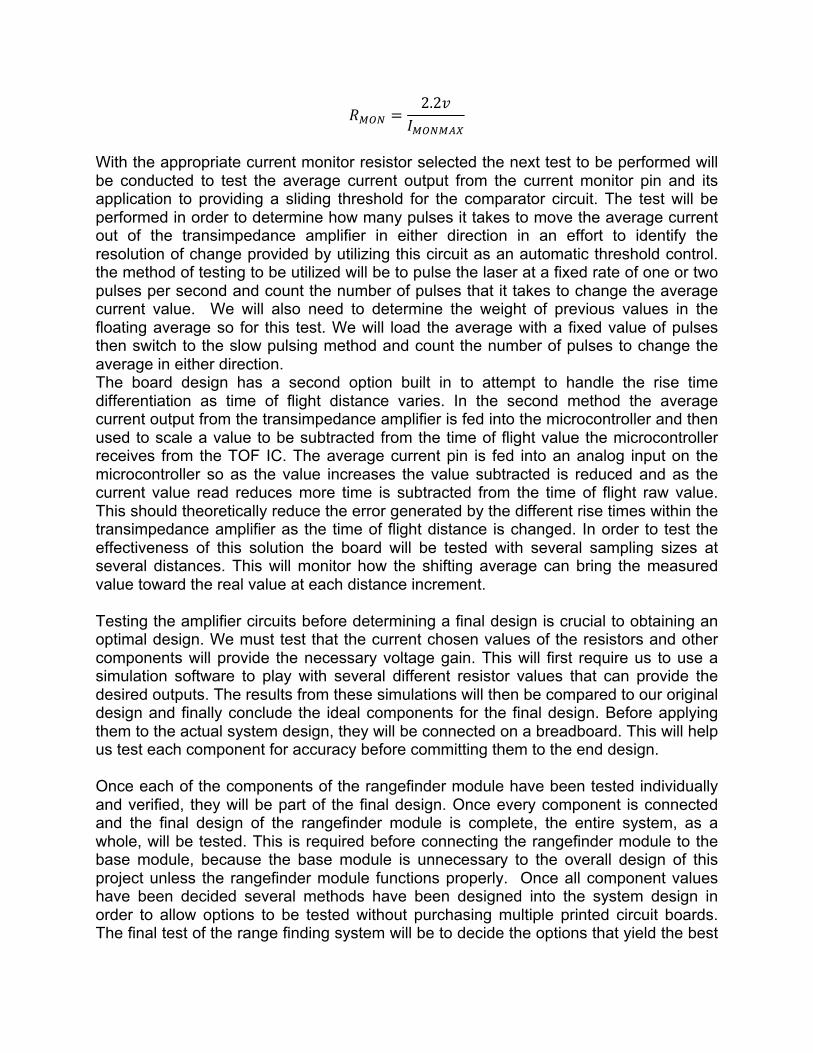
𝑅!"# =2.2𝑣

𝐼!"#!$%

With the appropriate current monitor resistor selected the next test to be performed will be conducted to test the average current output from the current monitor pin and its application to providing a sliding threshold for the comparator circuit. The test will be performed in order to determine how many pulses it takes to move the average current out of the transimpedance amplifier in either direction in an effort to identify the resolution of change provided by utilizing this circuit as an automatic threshold control. the method of testing to be utilized will be to pulse the laser at a fixed rate of one or two pulses per second and count the number of pulses that it takes to change the average current value. We will also need to determine the weight of previous values in the floating average so for this test. We will load the average with a fixed value of pulses then switch to the slow pulsing method and count the number of pulses to change the average in either direction. The board design has a second option built in to attempt to handle the rise time differentiation as time of flight distance varies. In the second method the average current output from the transimpedance amplifier is fed into the microcontroller and then used to scale a value to be subtracted from the time of flight value the microcontroller receives from the TOF IC. The average current pin is fed into an analog input on the microcontroller so as the value increases the value subtracted is reduced and as the current value read reduces more time is subtracted from the time of flight raw value. This should theoretically reduce the error generated by the different rise times within the transimpedance amplifier as the time of flight distance is changed. In order to test the effectiveness of this solution the board will be tested with several sampling sizes at several distances. This will monitor how the shifting average can bring the measured value toward the real value at each distance increment.

Testing the amplifier circuits before determining a final design is crucial to obtaining an optimal design. We must test that the current chosen values of the resistors and other components will provide the necessary voltage gain. This will first require us to use a simulation software to play with several different resistor values that can provide the desired outputs. The results from these simulations will then be compared to our original design and finally conclude the ideal components for the final design. Before applying them to the actual system design, they will be connected on a breadboard. This will help us test each component for accuracy before committing them to the end design. Once each of the components of the rangefinder module have been tested individually and verified, they will be part of the final design. Once every component is connected and the final design of the rangefinder module is complete, the entire system, as a whole, will be tested. This is required before connecting the rangefinder module to the base module, because the base module is unnecessary to the overall design of this project unless the rangefinder module functions properly. Once all component values have been decided several methods have been designed into the system design in order to allow options to be tested without purchasing multiple printed circuit boards. The final test of the range finding system will be to decide the options that yield the best

results therefore each of the options will be given a testing number within the schematics depicting that particular option the best result will be the option that yields a calculated measurement closest to the actual measurement in the fewest number of samples to get there.

5.4 Software Testing Software testing for the demonstration software, and all other software that is not firmware is very easy. The first step is to create a data server that emulates the data that would come from the scanning lidar. This is done by generating random points and then formatting them into packets the same way that the actual data server would. Once this is done, each individual module can be tested to make sure that it is functioning correctly. Most of the software modules are designed to be some kind of data visualizer so the test procedure for testing them will consist of viewing the graphical display and determining if it looks correct. If the LIDAR has already been built and tested, than the actual data server may also be used to test the other modules. This would be the ideal test conditions for the device because it would ensure that the data being displayed actually corresponds to data being read from the LIDAR. In addition to viewing the output data of the particular module, it is also important to make sure that multiple instances of the module can be running at the same time. The best test environment will have multiple computers so that the data server can be run on one computer and the other modules can be tested remotely. If everything is working correctly then there can be many instances of the different clients all running at the same time without interfering with one another. If the ideal situation where the LIDAR is actually present then additional tests can be performed. An object can be placed in front of the sensor and the shape of the object should be viewable the different visualization module. If the object does not show up on any of the visualizers, than there is probably either a problem with the data server, or a problem with the actual LIDAR. The latter is the most likely test case. If the data server is confirmed to have no errors than it is very likely that there is a problem with the Range Finding Module or the Base Module. See section 5.2 and 5.3 for testing these two modules.

6.0 Administrative Content

6.1 Milestone This intricate project required lots of time to configure a functional product that could be presented to a body of people. The steps involved in the entire process include defining the project, researching the components needed to accomplish the goals and specifications of the system, designing the system, prototyping the system, and finally testing the system. The next few sections outline the specific details and methods that were used by specifying the time management used throughout completion of this project. We were allotted five months to finish this project. Table 22 shows the overall milestone for each general step taken throughout this process.

Process Sections of Project

Due Date

June July August Sept Oct Nov

Define Initial Project

Document (Divide & Conquer)

June 5th

X

Specifications X

Research Table of Contents

June 30th

X

Rough Draft X X

Microcontroller X X

Base Module X X X

Rangefinder X X X

Power X X X

Software X X X X X X

Design Base Module X X

Rangefinder X X

Applications X X

Prototype Base Module X X X

Rangefinder X X X

Software X X X

Test System X X

Software X X Table 14 Timeline

6.1.1 June In the first month of being assigned this project, it was our goal to define the project. This began with an initial assignment of a one-page paper that required each of us to choose a project and determine what the project was, how we came up with the project,

what we wanted to accomplish with the project, and the specifications of the end result of the project. We each wrote about different projects for this paper, but when collaborating ideas for what we wanted to work on as a group, we agreed upon the Lidar device discussed throughout this paper. This was a project chosen by one of our group members for the initial assignment, which gave us insight when we had to explain our goals and motivations for this project. That brought us to our next task to complete in June which was determining the specifications we wished to accomplish with our system. Originally we wanted to make a LIDAR system that could not only scan an entire room, but also be able to map and even navigate through the room with the use of obstacle avoidance. Later, we determined that given the overall time and cost constraints we would have to narrow down our specifications to a more detailed and precise laser rangefinder that could gather distance data points and map them into a point cloud. This allowed us to have a general idea of what we needed to begin researching. Research began to allow us to complete and turn in the table of contents for this paper on June 30th. Little did we know then, there was a lot more to the project than we realized. 6.1.2 July The majority of the month of July was almost entirely spent doing research on LIDAR and laser rangefinders. From learning about similar devices and figuring out how to calculate distances to determining what components were needed to transmit and receive laser signal and how to go about interpreting those signals to produce actual data. None of our group members have ever designed a system quite like this one before, so the research was not only extremely important but also mandatory in order to start designing our system. Within researching throughout this month, it was our goal to have specific parts compared and analyzed for use for this system. We were able to justify almost all the parts we would need to accomplish the complete design. With specific parts picked out, we were able to complete the rough draft of this paper that was due sometime in the middle of this month. This allowed us to move into thinking about the tests that would need to be performed on the system to justify its function. 6.1.3 August The month of August began with finishing up this paper. That meant all design elements were chosen and testing the functionality of each component of the system and the system as whole was determined. By this time we also had a budget in place and a fairly good idea where we would acquire all of the parts needed. We finished the month off by designing the applications used to present the data that would be produced by the system. The first hurdle of this project was complete and we were fully prepared to jump the next hurdle. 6.1.4 September We used the entire month of September to buy all of the necessary components needed for our system. We knew some components would take longer to receive and we did not want to waste any time when it came to prototyping the system. As we started to acquire each piece, we tested them. This guaranteed that every piece not only worked as warrantied but also that they would all work properly for our design. We also began

testing the communication methods between the two microcontrollers. Using breadboards, oscilloscopes, and function generators we were able to begin testing each element individually and collectively. 6.1.5 October In October we focused on the accuracy and precision of our system. This allowed us to determine which components worked to create the specification previously defined and which ones were limiting us for achieving our goals. Based on these limiting components we were able to narrow down where exactly errors were originating and therefore adjusting parts to provide us with more accurate results. We also used this month to begin setting us the presentation material as well as printing out the PCB boards so we could begin building the actual system. We finished the month by completing the building process. 6.1.6 November We started the month of November with testing the functionality of our now completely built system. We needed to make sure there were no unforeseeable limitations before we could conclude that our system worked entirely. We also created more software to display the data produced by our system. This allowed for a more appealing representation of the results of the system for not only the group of people we were presenting to but also for friends and family that had less of an idea about what the system was designed to accomplish. 6.2 Budget The funding for our project will be all supplied by us. Keeping this in mind our ability to provide greater specifications was vastly. Our individual budgets were no more than $200. This provided us with an overall maximum budget of $800. Most time-of-flight laser sensors on the market range anywhere from $300.00 to a couple thousand dollars depending on the maximum range detection and other specifications. Based on this information and after researching specific parts that could be used in our design we initially estimated a total cost of $400.00. After finishing the design of the project, we determined the actual cost of the entire system to be approximately $250.00. This total cost includes the two microcontrollers, the motor and encoder, the motor mount, the shaft mount, the motor driver, the two PCB boards, the power supply, the optics, the laser diode, the photodiode, the time-to-digital converter, and an estimated cost of other small electronic components . These smaller electronic components include the resistors, capacitors, and other small devices needed to complete circuitry. This total cost does not include any shipping fees for parts or other fees that may be related to acquiring all the parts needed. It also does not include the labor costs that may arise as the system is being built. Table 23, below, lists the costs for each component.

Parts Quantity Cost ($)

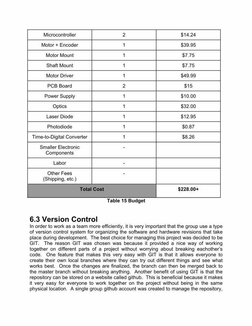
Microcontroller 2 $14.24

Motor + Encoder 1 $39.95

Motor Mount 1 $7.75

Shaft Mount 1 $7.75

Motor Driver 1 $49.99

PCB Board 2 $15

Power Supply 1 $10.00

Optics 1 $32.00

Laser Diode 1 $12.95

Photodiode 1 $0.87

Time-to-Digital Converter 1 $8.26

Smaller Electronic Components

-

Labor -

Other Fees (Shipping, etc.)

-

Total Cost $228.00+

Table 15 Budget 6.3 Version Control In order to work as a team more efficiently, it is very important that the group use a type of version control system for organizing the software and hardware revisions that take place during development. The best choice for managing this project was decided to be GIT. The reason GIT was chosen was because it provided a nice way of working together on different parts of a project without worrying about breaking eachother’s code. One feature that makes this very easy with GIT is that it allows everyone to create their own local branches where they can try out different things and see what works best. Once the changes are finalized, the branch can then be merged back to the master branch without breaking anything. Another benefit of using GIT is that the repository can be stored on a website called github. This is beneficial because it makes it very easy for everyone to work together on the project without being in the same physical location. A single group github account was created to manage the repository,

and then everyone created their own account so that everyone’s work could be documented better. In addition to using GIT as version control for the software development, it can also be used to organize the PCB design. This makes it much easier for the electrical engineers to modify the circuit boards, and track changes. The repository was set up to have two different folders, software and hardware. Everything that is related to software development and firmware was organized in the software directory. Everything that is related to hardware development, like PCB schematics and datasheets was placed in the hardware directory. Inside each of these folders, everything was further organized into demonstration, Base Module and Range Finding Module. Complications can occur when more than one person is working on the same files at the same time, so it is important that everyone in the group is in constant contact with one another. In situations where there are conflicts between different versions of the same file, a merge must be carried out. This will most likely require the group to meet up and discuss which version of the files help create the most reliable system. In order to keep things organized, the group adopted a set of best practices. The general rule was that whenever a new feature or change was to be made, create a new branch. All new changes are pushed to that branch and when the new feature is complete, the branch will be merged back with the master branch. By doing this, all changes to the software can be tracked and organized. After any kind of change has been completed, before it is merged with the master branch it is important that all other modules and features are properly tested in order to make sure that the changes did not break anything. Once the system is proven to be stable it is safe to merge the branch with the master.

7.0 Conclusion The lidar system design will be much cheaper than most available lidar systems that can be purchased. The reason this lidar design can be cheaper is because it does not have nearly as good performance as other available systems. The main area where more expensive lidar systems outperform this lidar is in scan rate. This design only allows for a scan rate of about 8 scans per second whereas many of the expensive systems are capable of upwards of 50 scans per second. This design is also not nearly as accurate as some of the available products which can have sub-centimeter accuracy. For hobbyists this is still a good option because most people do not have enough money for the high performance lidar systems currently available.

8.0 Bibliography 1. SLAM For Dummies (http://ocw.mit.edu/courses/aeronautics-and-

astronautics/16-412j-cognitive-robotics-spring-2005/projects/1aslam_blas_repo.pdf)

2. Arduino Laser Range Finder (http://forum.arduino.cc/index.php?topic=110549.0)

3. Webcam Based DIY Laser RangeFinder (https://sites.google.com/site/todddanko/home/webcam_laser_ranger)

4. OSLRF-01 Datasheet (http://www.lightware.co.za/shop/en/laser-sensors/24-oslrf-01.html)

5. Homemade Infrared Rangefinder Similar to SharpGP Instructable Project (http://www.instructables.com/id/Homemade-Infrared-Rangefinder-Similar-to-Sharp-GP/)

6.

A. Copyright Permissions

Hello Aaron,

Yes, you can use the figures. Please be sure to notate “CourtesyofTexasInstruments,Inc.”.

Regards Alexandria Davis Program Coordinator North America University Program Texas Instruments www.ti.com/university Email: univ@ti.com ================================================= TI makes no warranties and assumes no liability for applications assistance or customer productdesign.Youarefullyresponsibleforalldesigndecisionsandengineeringwithregardtoyourproducts,includingdecisionsrelatingtoapplicationofTIproducts.Byprovidingtechnical information,TIdoesnotintendtoofferorprovideengineeringservicesoradviceconcerningyourdesigns. [THREAD ID:1-UPOISM] -----Original Message----- From: aaron.smeenk@knights.ucf.edu Sent: 7/23/2015 03:53:52 PM To: "univ@ti.com" <univ@ti.com>

Subject: Senior Design permissions Hi, MynameisAaron,andIamcurrentlyworkingthroughmyseniordesignattheUniversityofCentralFlorida. Our project is LIDAR, and we are interested in utilizing your TDC7200 Time to DigitalConverter,IwaswonderingifIcouldusesomeofthefiguresfromthedatasheetinthedesignpaper. Thankyou Aaron Hyper Physics: Permission Pending ToRodNave@gsu.edu Hello, Myname is Keith and I ama current university studentworkingon a designpaper that includes asectiononmotors. Would it be okay if I include a cited image of one of the DCmotor diagrams currently posted onHyperPhysicswebpage? Thankyouforyourtime, Keith C.Z. Guan: Permission Given From:keith.hargett[keith.hargett@knights.ucf.edu] Sent:Tuesday,August04,20155:19PM To:CharleszGuan Subject:DiagramUsage Itwasadiagramshowingthewindingsonabrushlessmotor. Thanks ________________________________________ From:CharleszGuan<charlesg@mit.edu> Sent:Tuesday,August4,20155:15PM To:keith.hargett Subject:RE:DiagramUsage Whichdiagramareyoutalkingabout? Eitherwayit'sprobablyfinelol CharlesZ.Guan Instructor,PostmodernRobotics MIT-SUTDCollaboration,MIT ________________________________________ From:keith.hargett[keith.hargett@knights.ucf.edu]

Sent:Tuesday,August04,20155:14PM To:CharleszGuan Subject:DiagramUsage Hello, MynameisKeithandIamacurrentuniversitystudentwritingadesignpaperthatincludesasectiononmotorcontrol. InoticedamotordiagrampostedonanInstructablesprojectandIwaswonderingifitwouldbeokayformetouseacitedimageofthediagram. Thankyouforyourtime, Keith RP Photonics: Permission Given DearMr.Hargett, You can use some images are text sections from ourwebsite, provided that you properly cite theoriginofthesematerials:EncyclopediaofLaserPhysicsandTechnologyfromRPPhotonicsConsultingGmbH,http://www.rp-photonics.com/mode_locked_lasers.html Withbestregards RüdigerPaschotta On2015-08-0500:44,keith.hargettwrote: Hello, MynameisKeithandIamacurrentuniversitystudentwritingadesignpaperthatincludesasectiononmode-lockedlasers. Would it be okay if I used a cited image of the passive and active mode locked laser diagramscurrentlypostedonyourwebsite? Thankyouforyourtime, Keith SPIE: Permission Pending Tocustomerservice@spie.org Hello, MynameisKeith,IamauniversitystudentandIamcurrentlywritingadesignpaperthatincludesasectiononmode-lockedlasers. WoulditbeokayifIuseacitedimageofthepulsediagramyouhaveonyoursite?

Thankyouforyourtime, Keith Battery Univeristy: Permission Given To:keith.hargett; HiKeith Yes,youmayusethematerialasrequested.Pleasecitesourceswhereappropriate. Regards, JohnBradshaw-MarketingCommunicationsManager CadexElectronicsInc.|www.cadex.com >>>"BatteryUniversity"<web@batteryuniversity.com>8/4/20152:03PM>>> SomeonehassubmittedaBatteryUniversitycontactform. Herearethedetails: EntryDate:2015-08-0402:03PM FirstName:Keith LastName:Hargett Email:keith.hargett@knights.ucf.edu Comments:HelloIamauniversitystudentandIamwritingadesignpaperthatincludesasectiononbatteries.WoulditbeokayifIincludeacitedimageofthetablethatdiscussesrechargeablebatterieswithinmyreport? Thankyouforyourtime, Keith Radio Electronics: Permission Pending HelloIamauniversitystudentandIamwritingadesignpaperthatincludesasectiononseriesandshunt regulators.Would it beokay if I includea cited imageof the table that coversDC regulatorswithinmyreport? Thankyouforyourtime, Keith Texas Instruments: Permission Pending To:copyrightcounsel@list.ti.com; DearCopyrightDepartment,

IamacurrentuniversitystudentworkingonadesignpaperthatinvolvesDCregulators. Would it be okay if I used a cited image of a few regulator circuits currently on TI's instructionalmaterial? Thankyouforyourtime, Keith