Embed Size (px)
Citation preview

3 9
C H A P T E R 3
Laser Telemeters
A telemeter is an instrument for measuringthe distance to a remote target. Basically, the three main techniques to perform an opticalmeasurement of distance are the following:
- Triangulation. The target is aimed at from two points separated by a known base D,placed perpendicular to the line of sight. By measuring the angle α formed by thetwo line of sights, the distance is found as L=D/α.
- Time of flight. A light beam from a high-radiance source is propagated to the target andback, and the time delay T=2L/c is measured (c is the speed of light). The distancefollows as L=cT/2.
- Interferometry. A coherent beam is used in the propagation to the target. The returnedfield is detected coherently by beating with a reference field on the photodetector,and a signal of the form cos 2ks (where k=2π/λ) is obtained. From cos 2ks, wecan count the distance increments in units of λ/2.
In view of the obtained performances, the three approaches are complementary.Triangulation is the simplest technique to implement and may operate in daylight even
without any source. Until a few decades ago, it survived in construction applications withthe theodolite (to measure α) and the rulers (to set D). However, it has a poor accuracy onlong distances because, when L is much larger than the base D, the angle α to be measuredbecomes very small and is affected by errors.

4 0 Laser Telemeters Chapter 3
The time of flight technique requires a pulsed or a sine-wave modulated laser. In bothcases, we measure the time of flight T=2L/c of light to the target at distance L. This teleme-ter works with a constant accuracy ∆T (or, in distance, ∆L=c∆T/2), in principle. Thus, per-formance is excellent on medium and long distances. Because of this, it has superseded thetheodolite on medium distances (100 m to 1 km) and has proven to be a new powerful tech-nique in a number of long-distance (greater than 1 km) applications.
Last, the interferometric technique is by far the most sensitive, but has the drawback ofrequiring the development of the λ/2-counts by a movement of the target. Thus, this tech-nique provides basically an incremental measurement of distance, not an absolute one as theother two techniques. For this reason, interferometric techniques are treated separately inChapter 4, whereas in this chapter we will concentrate mainly on time of flight telemeters.
From the point of view of the remote target features, we may have either (i) a coopera-tive target made of a retroreflector surface to maximize the returning signal (ii) a noncoopera-tive target, simply diffusing back the incoming radiation with a δ<1 diffusion coefficient.
According to the measurement technique employed, time of flight telemeters are classi-fied as one of the following:
- Pulsed telemeters when the measurement is performed directly as the delay T betweentransmitted and received pulses
- Sine-wave modulated telemeters, when the source is modulated in power by a sine waveat a frequency f, and the delay T is measured from the phase Φ=2πfT.
The first case relates to long-range telemeters and is useful for geodesy research and militaryapplications, with operational ranges up to 100 km or more, whereas the second identifiesthe topographic telemeters used on medium ranges (<1km) for civil engineering and con-struction work applications.The laser sources most suitable in the two cases are the following:
- Solid state lasers (like Nd, YAG) operated in the Q-switching regime and semiconduc-tor-diode (like GaAlAs) arrays, pulsed at 1 to 10-ns durations
- Quasi continuous-wave semiconductor lasers like GaAlAs and GaInP to supply modu-lation up to hundreds of MHz.
3.1 TRIANGULATION
Let us consider the basic scheme for triangulation illustrated in Fig.3-1. Here, a distantobject O is aimed from two observation points, A and B, along a base of width D.The object is assumed self-luminous for the moment, which is a case referred to as passivetriangulation. Active triangulation using a laser source to illuminate the target is consideredlater on.
The beamsplitter and rotatable mirror combination allows superimposing the imagesseen at A and B. The mirror M is rotated by an angle α from the initial position α=0 paral-lel to the beamsplitter until the object images are brought to coincide. The distance L thenfollows as:
3.1 Triangulation 4 1
Fig. 3-1 Basic scheme of a triangulation measurement
L = D / tan α ≈ D / α (3.1)
Of course, we need a good measurement of small α to determine a long distance L with areasonably short base D. The absolute and relative errors, ∆L and ∆L/L, due to an angle error∆α, are found from Eq.3.1 as:
∆L = - (D/α2) ∆α = - (L2/D) ∆α (3.2)
∆L /L = - (L/D) ∆α (3.2’)
and they both increase with distance. For design purposes, the errors are plotted in Fig.3-2 asa function of L and with ∆α as a parameter.
With regards to the error of the angle readout, a good micrometer screw with gear re-duction and backlash recovery is representative of medium-accuracy performance and mayresolve ∆α=10 arc-min (≈3 mrad). On the other hand, an angle encoder may provide a high-accuracy readout, going down to the limit of the (small) viewing telescope, typically∆α=0.3 arc-min (≈0.1 mrad).
In these two representative cases, it is interesting to evaluate the performance of theoptical telemeter based on triangulation. Let us exemplify the results for two hypotheticaltelemeters, one intended for short distance (L≈1m) and the other for medium distance (say100 m).
At a distance of L=1 m, we may choose a D=10-cm base as a reasonable value for acompact instrument. From Fig.3-2, we find the intrinsic accuracy as ∆L/L=3% and 0.1%,respectively for ∆α=3 and 0.1 mrad. Turning to the 100-m telemeter, we may expand thebase within the limits allowed by the application and perhaps go to D=1m. Then, fromFig.3-2, we find ∆L/L=30% and 1% for ∆α=3 and 0.1 mrad.
α
object O
α
L
A
B
telescope beamsplitter
Mrotatable mirror
D

4 2 Laser Telemeters Chapter 3
Fig. 3-2 Distance accuracy (relative ∆L/L and absolute ∆L) in triangulation meas-urements. Entering with ∆α and D values in the upper right corner diagram(see small-dot line for 0.1 mrad and 1m) gives the parameter ∆α/D andhence the relative accuracy ∆L/L versus distance. Large-dot lines sup-ply the absolute distance accuracy ∆L. Because the approximationtanα≈α has been used, the diagram is valid for D<<L.
As it is clear from these examples, triangulation can achieve respectable performance,provided the application allows using a not-too-small base-to-distance ratio D/L.
A triangulation telemeter can be developed straight from the basic concept outlined inFig.3-1. Such an instrument is classified as a passive optical telemeter because it does notrequire a source of illumination or a detector.
However, if we add a source to aim the target and a position-sensitive detector to sensethe return, we can improve performance, eliminate the moving parts, and get a faster re-sponse. The best scheme for the active triangulation scheme can take very different configu-rations, depending on the requirements of the specific application (e.g., dynamic range, accu-racy, size, and cost) [1].To substantiate a design example, we report in Fig.3-3 the layout of an active triangulationtelemeter intended for short distances (1 to 10 m) that uses a semiconductor laser and a CCD.
10
1
0.1
0.1110∆α (mrad)
base D(m)
0.01 0.11 cm
10
0.1
1
∆α /D= 0.01 mrad/m
-210
-110
-410
-310
101 100 1000distance L (m)
relativeaccuracy ∆L/L
absolute accuracy
∆L =10 cm
3
3
3
.1
3
3
3 3 3
3
30 3

3.2 Time-of-Flight Telemeters 4 3
The laser wavelength is chosen in the visible for ease of target aiming, and the power is usu-ally a few mW emitted from an elliptical near-field spot of 1×3 µm size (typically).An anamorphic objective lens circularizes the beam to a radius wl (typ. 5µm) and projects animage of it on the target.On the target, the spot size radius is then wl L/Fill (=5µm×1000/125=40µm for L=1m andFill =125mm). As a viewing objective, we use a telephoto lens with focal length Frec (typi-cally 250 mm) and get an image of the target on the CCD.The CCD (see [2], Sect.9.2] is a silicon device composed of a linear array of N individualphotosensitive elements of width wCCD (typically, we may have N=1024 and wCCD= 10µm).The size of the target-spot that is imaged on the CCD by the objective is easily computed aswl L/Fill (Frec/L)= wl Frec /Fill =5µm×250/125=10µm, which is equal to the pixel size wCCD.We may assume that the accuracy of localization in the focal plane is limited by the pixelsize (see Ref.[3] for a refinement that takes into account speckle errors). Then, the angularresolution is ∆α= wCCD/Frec =10µm/250 mm =0.04 mrad. By taking an axis separationD=50 mm, and from the data in Fig.3-2 we have ∆L/L=0.1% at L=1 m, and ∆L/L=1% atL=10 m.Converted in absolute errors, our telemeter would resolve 1mm at 1m and 10cm at 10m, andperhaps the results may be still improved.
Fig. 3-3 Scheme of a triangulation telemeter with active illumination and a staticangle readout. The optical axes of illuminating and viewing beams areparallel. The target-spot image is formed off-axis at a distance αFrec,where Frec is the focal length of the viewing objective. An Interference Fil-ter (IF) is used for ambient light rejection.
3.2 TIME-OF-FLIGHT TELEMETERS
These telemeters are based on the measurement of the time of flight T=2L/c of light tothe target at distance L and back. The uncertainty ∆T of measurement reflects itself in a dis-tance uncertainty ∆L=c∆T/2. Accordingly, if we are using a pulsed light source, we require
LASER
target
α
IF
D
CCD

4 4 Laser Telemeters Chapter 3
that the pulse duration τ be short enough for the desired resolution, or τ<∆T.Similarly, if we use a sine-wave modulated source, the frequency of modulation ω needs tobe high enough, or ω>1/ ∆T.
In the following sections, we first study the power budget of a generic time of flighttelemeter, then evaluate the ultimate distance performance of pulsed and sine-wave modulatedapproaches, and conclude with the illustration of several schemes of implementation [4].
3.2.1 Power Budget
The power budget of a time of flight telemeter can be analyzed with reference to Fig.3-4.The optical source emits a power Ps, and the objective lens projects it on the target with anangular divergence θs= Ds/Fs, where Ds is the diameter of the source and Fs is the focallength of the objective lens. A detector is aimed to the target through a receiving objectivelens with diameter Dr.We will consider the target either as cooperative (a corner cube for self-alignment) or nonco-operative (to account for a normal diffusing surface, with diffusivity δ<1).
When the target is cooperative, the corner cube acts as a mirror, so the receiver sees thesource as if it is at a distance 2L. Accordingly, the power fraction collected by the receiver isthe ratio between the area of the collecting lens and the area of the transmitted spot at a dis-tance 2L:
Fig. 3-4 General scheme for evaluating the received power Pr in a telemeter as afunction of transmitted power Pt, distance L, and transmitter/receiver op-tics. The target may be either a corner cube or a diffuser. Because thedistance L is much larger than other dimensions in the drawing, the fieldof view is actually superposed on the field of illumination.
diffuser (non-cooperative)
corner cube(cooperative)
source
ds
dr
s
s
detector
r
F
Fr
D
D
transmitterobjective lens
receiverobjective lens
P
Pr
s
sθ
L
target

3.2 Time-of-Flight Telemeters 4 5
Pr /Ps = Dr2 /(θs
2 4L2) (3.3)
Eq.3.3 holds if the corner cube diameter Dcc is large enough and does not limit collection ofradiation at the receiver. This requires that Dcc ≥Dr/2. If the reverse is true, we shall use Dccin place of Dr/2 in Eq.3.3.
When the target is noncooperative, that is, a diffusing surface of area At, the power ar-riving on the target is Ps, and a fraction δ of it is rediffused back to the receiver.Assuming a Lambertian diffuser, the radiance R of the target is 1/π times the power densityδPs/At, or R= δPs/πAt. Accordingly, the power collected by the receiver is RAtΩ, whereΩ is the solid angle of the receiver seen from the target, given by Ω=Dr
2/4L2. Thus, wehave:
Pr /Ps = δ Dr2/4L2 (3.4)
Also in this case, if the target has a diameter Dtar smaller than θsL, the Pr /Ps ratio is reduced
by a factor (Dtar/θsL)2, and the dependence on distance would then become of the type L-4, asfor a microwave radar. In the following, we restrict ourselves to the case Dtar>θsL.
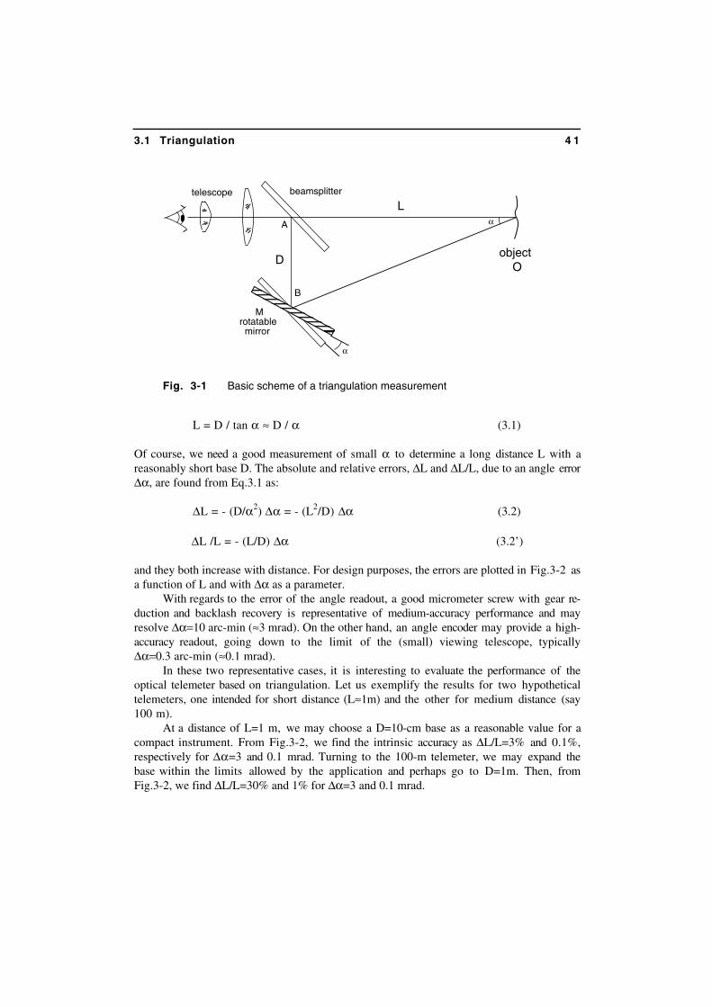
Eqs.3.3 and 3.4 describe the attenuation due to geometrical effects only. We may alsofind an additional contribution from the transmittance Topt of the transmitter/receiver lenses,and from the propagation through the atmosphere with an attenuation Tatm=exp-2αL, whereα is the attenuation coefficient of the air (see Appendix A3.1). We can account for theseterms by multiplying the second members of Eqs.3.3 and 3.4 by ToptTatm so that we have ingeneral:
Pr /Ps = ToptTatm Dr2 /(θs
2 4L2) (3.3’)
Pr /Ps = δ ToptTatm Dr2/4L2 (3.4’)
As a rule of thumb, we may take α=0.1km-1 for an exceptionally clear atmosphere,α=0.33 km-1 for a limpid atmosphere, and α=0.5km-1 for an incipient haze. The correspond-ing values of Tatm are reported in Fig.3-5 for medium/long ranges.The previous values are an average in the range of visible wavelengths. However, becausethe telemeter will operate at a well-defined wavelength, it is important to have a closer lookto the spectral attenuation α=α(λ).
Information on α=α(λ) is provided by Fig.A3-2 of Appendix A3. In addition, compara-tive data can be gathered from the spectrum of the solar irradiance, see Fig.A3-3. From here,we can see that there are some wavelengths to be avoided (e.g. 0.70, 0.76, 0.80, 0.855, 0.93and 1.13 µm) because they coincide with absorption peaks of the atmosphere. On the otherhand, wavelengths like 0.633 (He-Ne), 0.82..0.88 (GaAlAs), and 1.06 µm (Nd) are accept-able for long-range telemeters.
Now, we can generalize the power–budget equations by introducing an equivalent dis-tance Leq=L/Tatm and a gain factor G, so that:
4 6 Laser Telemeters Chapter 3
Fig. 3-5 Atmospheric transmittance as a function of target distance, with the at-tenuation coefficient as a parameter.
Pr /Ps = G Dr2 /4Leq
2 (3.5)
By comparing with Eqs.3.3 and 3.4, G is given by:
G = Gnc = Topt δ (noncooperative target) (3.6a)
G = Gc = Topt/θs2 (cooperative target) (3.6b)
With this position, Eq.3.5 is the power-attenuation equation and tells us that the Pr/Psratio depends on the inverse square of target distance or, better, from the ratio (Dr/L)2.
On the other hand, Eqs.3.6a and b are about the gain of the target, either cooperative ornoncooperative.The cooperative gain Gc is the counterpart of the antenna gain known in microwave, and isgiven by the inverse squared of the divergence angle, 1/θs
2. This factor may be very largeindeed (for example, it is Gc=106 for θs=1 mrad).
3.2.2 System Equation
Let us consider the system performance of the telemeter. If Pr is the received power andthe receiver circuit has a noise Pn, we shall require that the ratio of the two, i.e.:
1
10-2
10-4
Tatm
atmospherictransmittance
0 5 10 15 20
target distance L (km)
α = 0.05 km-1
0.2
0.5
0.1
0.3
=exp -2αL

3.2 Time-of-Flight Telemeters 4 7
S/N = Pr /Pn, (3.7)
is at least, say 10, to get a good measurement. By combining Eqs.3.7 with Eq.3.5 we get:
GPs = Pr 4Leq2/Dr
2
= (S/N) Pn 4Leq2/Dr
2 (3.8)
Eq.3.8 is the system equation of the telemeter because it relates the required S/N ratioto receiver noise Pn and to attenuation 4Leq
2/Dr2. The diagram of the equivalent power GPn
versus distance Leq and with the receiver noise Pn as a parameter is plotted in Fig.3-6.
Fig. 3-6 Graph of the transmitted equivalent power versus normalized distance,with the receiver noise power as a parameter. It is assumed a S/N=10 anda receiver objective with Dr=100 mm. Zone 1 is representative of a sine-wave modulated topographic meter and zone 2 of a pulsed telemeter.
1
1 mW
1 nW
1 µW
1 pW
101 1000.1
re
ceive
r
noise
pow
er
nP =
2
rS/N = 10D =100mm
normalized distance L/√T (km)atm
1m
1
1k
1M
equivalent power G P (W)
s
4 8 Laser Telemeters Chapter 3
Two central-design regions are indicated in Fig.3-6. One representative of a sine-wavemodulated telemeter for topography, which may use a ≈1 mW transmitted power and hasGPs≈ 1W in virtue of the cooperative target (corner cube) gain. Because the measurementtime T can be long (e.g., 10ms to 1s), the bandwidth B=1/2T is small, and the receiver noisecan go down to the nW’s level.
The second case is representative of a pulsed telemeter intended for noncooperative tar-gets. The source is likely to be a Q-switched laser with a high peak power (≈0.1-1MW, re-sulting from ≈mJ energy per pulse and τ≈10ns pulse duration). Using a pin/APD photodiode(see [2], Ch.4) as the detector, and taking into account that the bandwidth B≈1/τ is nowmuch larger, the receiver noise is in the range of the µW’s.
We have three contributions to add about receiver noise, namely:
- noise of the received signal Ps- noise of the background light Pbg collected by the receiver- noise of detector and front-end amplifier
To describe noise, we use the standard deviation pn of the fluctuations referred to the de-tector input, a quantity called the Noise-Equivalent-Power (NEP) (see Ch.3 of Ref.[2]).As a reasonable assumption, we assume that the photons of both signal and backgroundlight obey the Poisson statistics. Upon detection, each photon is converted into an electronwith a success probability η, which is called a Bernoulli process. The photon flux Fph isthus transformed in an electron flux Fel =ηFph, where η is the quantum efficiency of the de-tector. It can be shown that the cascade of a Poisson and a Bernoulli process is a Poissonprocess. Thus, the detected electrons follow the Poisson statistics, and the associated currenthas fluctuations described as shot noise with a white spectral density. Now, the average de-tected currents are written as Is =σPs and Ibg=σPbg, where σ=ηe/hν is the spectral sensitivityof the detector (Ref.[2], Ch.4). Superposed to the average currents, we find shot noise fluc-tuations ins and inbg whose variances are given by ins
2=2eIsB and inbg2=2eIbgB, with B being
the bandwidth of observation.The detector and front-end noise are summarized by an equivalent characteristic current
Iph0 (see [2], Ch.3), defined as the current value for which the shot-noise is equal to the totalnoise of detector and front-end, that is inph0
2=2eIph0B.Summing up the contributions (because they are mutually uncorrelated), the total vari-
ance of the detector current is irec2 = inph0
2+ins2+inbg
2, or:
irec2 = 2eB (Is+ Ibg+ Iph0) (3.9)
We can divide irec2 by σ2, the spectral sensitivity (coincident, in this case, with the re-
sponsivity), to get the (total) noise power variance at the input:
pn2 = (2hν/η) B (Ps+ Pbg+ Pph0) (3.10)
In this equation, we have let Pph0=Iph0/σ for the power corresponding to Iph0. An extra1/η factor is left over in Eq.3.10 after the σ’s ratios of powers to currents have been clearedand 2hνσ has been transformed in 2e.

3.2 Time-of-Flight Telemeters 4 9
This is the correct result, however, because a real detector with η<1 worsens the S/N ratio ofdetected current by η respect to the S/N of incoming power.
The noise performances obtained by several combinations of detector and front-end pre-amplifiers are discussed in detail in Ref.[2], Ch.4. As a guideline for the reader, we summa-rize in Fig.3-7 the performance we may reasonably expect from a well-designed receiver forinstrumentation applications.
Data are given in terms of the current noise spectral density in/√B, as a function of themaximum frequency of operation of the receiver f2 (that is, of the cutoff frequency). To ob-tain pn, the value read in Fig.3-7 shall be multiplied by the square root of the measurementbandwidth and divided by σ√η (Eq.3.10).
Fig. 3-7 Typical noise performance of receivers, as a function of the maximum fre-quency of operation f2. Silicon-photodiodes with FET- and BJT- transistorinput-stage (with eventual equalization correction) are compared to ava-lanche photodiodes (APD) and to photomultipliers (PMT). Si-photodiodescover the range λ=400-1000nm, whereas InGaAsP extend up to ≈1.6µmand standard PMTs are centered in the range 300 to 900 nm. Data are for adetector with area A<0.5mm2 and capacitance C<0.5pF, and front-endswith FET and BJT having a transition frequency fT≥2GHz.
100 M 1G
nois
e sp
ectr
al d
ensi
ty I
/√B
(p
A/√
Hz)
n
0.01
0.1
1
10
maximum frequency f (Hz)2
1M 10M
Si-pin + FET
Si-pin + BJT
InGaAsP-pin + IC
InGaAsP APD
Si-APD
PMT

5 0 Laser Telemeters Chapter 3
To evaluate the term Pbg in Eq.3.10, we shall consider the spectral irradiance Es(W/m2µm) of the scene on which the telemeter is aimed.In daytime with direct sunlight illumination at different elevation angles, Es is given by thediagram of Fig.A3-3. In other conditions (clouds, haze, etc.), the same diagram can be usedas a first approximation, by properly rescaling the curve amplitude.
From the law of photography (App.A2, Ref.[2]), we can write the power collected atthe receiver objective lens as:
Pbg = δ Es ∆λ NA2 (π dr
2/4) (3.11)
where:
δ = scene diffusivityEs = scene spectral irradiance (W/m2µm)∆λ = spectral width of the interference filter placed in the receiver lensNA = arcsin Dr/2F = numerical aperture of the receiver lensdr = diameter of the detector
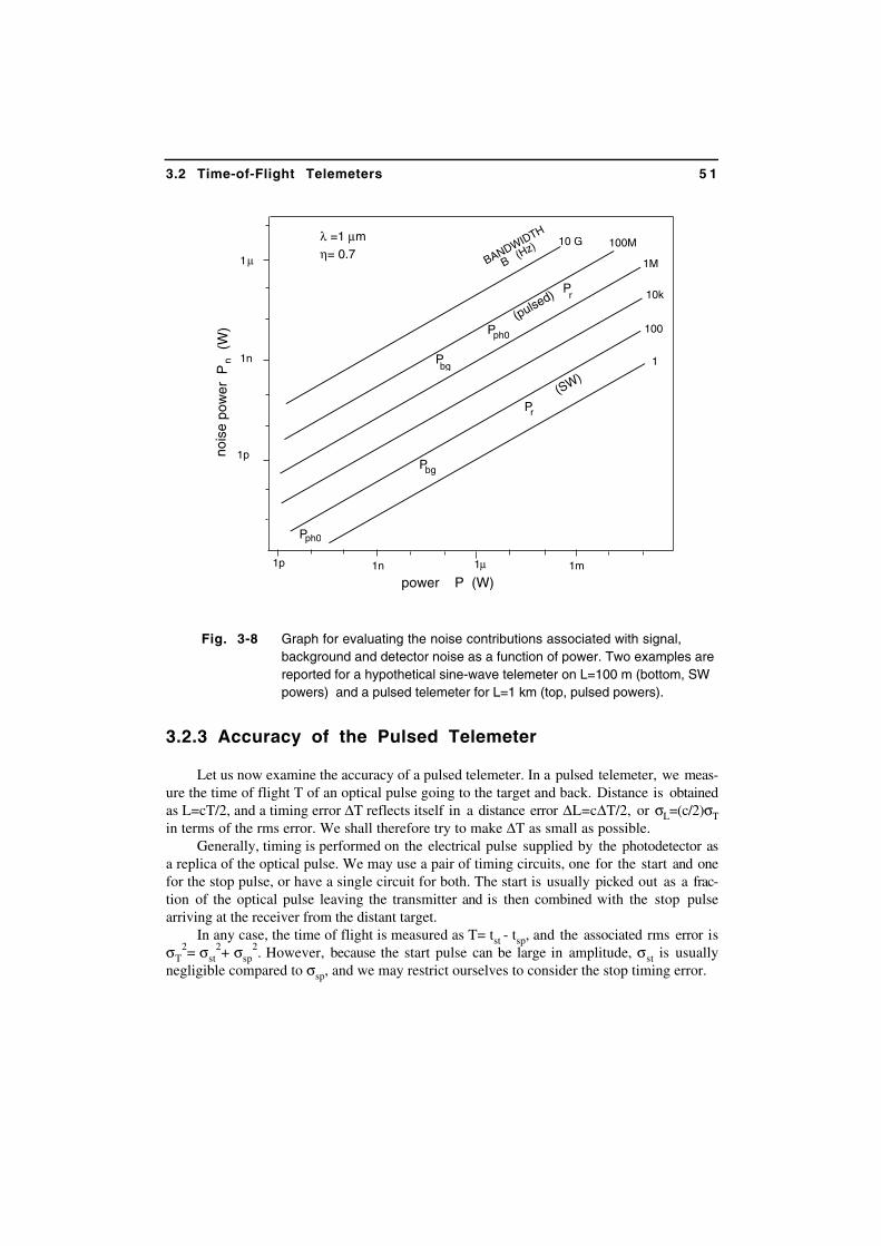
To compare the relative importance of the noise terms, we can use the diagram ofFig.3-8, which is a plot of the quantity pn=√[(2hν/η)PB] for λ=1µm and η=0.7. Let us substantiate the previous considerations with the aid of numerical examples for apulsed telemeter and a sine-wave telemeter.
For a Nd-laser pulsed telemeter operating at λ=1060 nm, we may have (Fig.A3-3) Es≈500 W/m2µm in direct sunlight at AM1.5 (sun elevation 42°). Other common design valueswe may assume are ∆λ=10nm (for an 80 to 90% transmission of the filter), NA=0.5, anddr=0.2 mm. Taking δ=1 as the worst case for background and inserting in Eq.3.11, we getPbg=40 nW.The attenuation is Pr/Ps= δ(Dr/2L)2. Working at L=1 km with Dr=100 mm and δ=0.3 for thesignal, we have Pr/Ps= 0.075 10-8, that is, for a typical transmitted (peak) power of Ps =0.3MW, we get a received power Pr=0.23 mW. In addition, the Iph0 noise for an APD receiver at100 MHz is evaluated from Fig.3-7 as 2 pA/√Hz. Multiplying by √B/η√σ, we get Pph0≈4nW. Thus, we obtain the points labeled ‘pulsed’ in Fig.3-8, and we can see that it is thereceived signal shot-noise to prevail.
For a sine-wave modulated telemeter operating at λ=820 nm, we may have Es≈ 900W/m2µm and Pbg approximately doubles at a value of 80nW.The attenuation is now Pr/Ps= Dr
2/4θs2L2. Working at L=100 m with Dr=100mm and θs=1
mrad, we have Pr/Ps= 0.25. That is, for a typical transmitted power of Ps =0.1 mW, we get areceived power Pr=25 µW.Again, using an APD receiver at 10 MHz, the noise spectral density is 0.2 pA/√Hz, andmultiplying by √B/η√σ with a bandwidth of 100 Hz now, we get Pph0≈5 pW.
In both cases, the largest term is the shot-noise of the received photons. This corre-sponds to a good-design result. On the contrary, if we had omitted the filter for the back-ground or used too large a detector or noisy electronics, the Ibg or Iph0 values could easily beincreased by order of magnitude and become the limiting factor of telemeter performance.
3.2 Time-of-Flight Telemeters 5 1
Fig. 3-8 Graph for evaluating the noise contributions associated with signal,background and detector noise as a function of power. Two examples arereported for a hypothetical sine-wave telemeter on L=100 m (bottom, SWpowers) and a pulsed telemeter for L=1 km (top, pulsed powers).
3.2.3 Accuracy of the Pulsed Telemeter
Let us now examine the accuracy of a pulsed telemeter. In a pulsed telemeter, we meas-ure the time of flight T of an optical pulse going to the target and back. Distance is obtainedas L=cT/2, and a timing error ∆T reflects itself in a distance error ∆L=c∆T/2, or σL=(c/2)σTin terms of the rms error. We shall therefore try to make ∆T as small as possible.
Generally, timing is performed on the electrical pulse supplied by the photodetector asa replica of the optical pulse. We may use a pair of timing circuits, one for the start and onefor the stop pulse, or have a single circuit for both. The start is usually picked out as a frac-tion of the optical pulse leaving the transmitter and is then combined with the stop pulsearriving at the receiver from the distant target.
In any case, the time of flight is measured as T= tst - tsp, and the associated rms error isσT
2= σst2+ σsp
2. However, because the start pulse can be large in amplitude, σst is usuallynegligible compared to σsp, and we may restrict ourselves to consider the stop timing error.
1M
1µ1n 1m1p
BANDWIDTH
B (H
z)
power P (W)
100
10k
1
100M
1µ
1n
1p noi
se p
ower
P
(W
)n
λ =1 µmη= 0.7
10 G
(SW)
(pulsed)
Pbg
Pph0
Pr
Pbg
Pph0
Pr

5 2 Laser Telemeters Chapter 3
Several approaches and circuit solutions are available to implement time measurementson pulses. Most of them are based on threshold crossing, as illustrated in Fig.3-9. An ampli-tude discriminator with a threshold S0 is used. Well-known circuit implementations for it arethe Schmitt trigger, the tunnel-diode trigger, and other fast circuits.
When the signal crosses the threshold, the circuit switches and gives a step-wise wave-form at the output. The circuit adds a negligible jitter in switching time (<10ps in a well-designed circuit). Thus, the timing fluctuation σt
around the average time t0 is only due topulse noise, specifically to the fluctuations σS on the mean amplitude waveform S(t).
Fig. 3-9 Timing of the received pulse by means of an amplitude discriminator.When the signal crosses the threshold S0 at time t0, a timing signal isgenerated. Amplitude fluctuations ±σS produce a timing error ±σt.
The error in time σt can be related to the error in amplitude σS through a linear regres-
sion, by writing:
σt2 = σS
2 /⎮ dS/dt⎮2 (3.12)
The linear regression is accurate when the amplitude fluctuation σS is small and the signal
slope dS/dt is nearly constant in the crossing region, which is a reasonable hypothesis inmost cases.
Now, let us now introduce normalized variables to get a better insight into the prob-lem. The received pulse is written as a power:
S(t)= Er (1/τ) s(t/τ) = Pr(t) (3.13)
S(t) + σ (t)s
sS(t) - σ (t)
S0
σ t0t +σ0 tt - t0
S(t) mean signal
output from the trigger circuit
3.2 Time-of-Flight Telemeters 5 3
where- τ is the time parameter (or scale) of the pulse, approximately equal to its duration;- s(t/τ) is the dimensionless pulse waveform, with a peak value speak≈1 and an area normal-
ized to unity, i.e., ∫0-∞ (1/τ)s(t/τ)dt=1. The frequency spectrum of s(t/τ) extends up toB≈κ/τ, with κ being a numerical factor usually not far away from 1/2π=0.16;
- Er is the energy contained in the pulse, as implied by the normalization of s(t/τ).With these positions, the signal slope is dPs(t)/dt =Er (1/τ2)s’(t/τ). Using Eq.3.10 for
the amplitude variance in Eq.3.12 and with Eq.3.13, we have:
σt2 = (2hν/η) (κ/τ) [Er (1/τ)s(t/τ)+Pbg+Pph0]/[Er(1/τ2)s’(t/τ)]2
= τ2 (2hν/η) κ [s(t/τ)/Er +(Pbg+Pph0) τ/Er2]/s’2(t/τ) (3.14)
This expression tells us that the accuracy σt is primarily proportional to the pulse durationτ. In addition, by writing it in the form:
σt = τ (A hν/Er + B/Er
2)1/2 (3.15)
where A and B are appropriate terms, we can see that the first term contributes to accuracy as√(hν/Er)=1/√Nr, which is the inverse square root of the number Nr of received photons. In a well-designed receiver, the shot noise hν/Er term should dominate over the othernoises, and the second term in parentheses should be negligible. In this case, we have:
σt ≈ τ /√Nr (3.16)
By introducing Nr in Eq.3.14,we obtain the general expression:
σt = τ/√Nr [(2κ/η) s(t/τ)/s’2(t/τ)]1/2 [1+τ(Pbg+Pph0)/s(t/τ)Er]
1/2 (3.16’)
From this expression, we can see that, besides the main dependence on τ/√Nr, the ef-fects of quantum efficiency and pulse waveshape are summarized by the factor √2κ/η. Also, the accuracy depends on the relative square slope s’2(t/τ)/s(t/τ), a dimensionlessquantity less than, but not so far from unity, whose actual value is determined by the se-lected threshold S0=s(t/τ). Of course, we will choose S0 so that the threshold-dependent factors’2(t/τ)/s(t/τ) is maximum. Finally, if background and electronics noises are not negligible, their effect worsens theideal accuracy by the factor in square parentheses in Eq.3.16’.This factor can also be written as [1+Nbg+ph0/S0Nr]
1/2, where Nr is the total number of pho-tons in the pulse, S0Nr is the number of photons collected at the threshold crossing time,and Nbg+ph0=τ(Pbg+Pph0)/hν is the number of photons equivalent to background front-endpowers Pbg and Pph0 collected in a pulse-duration time τ.Explicitly, we may rewrite Eq.3.16’ as:
σt = τ/√Nr [(2κ/η) S0/s’2(t/τ)]1/2 [1+Nbg+ph0/S0Nr]
1/2 (3.16’’)
5 4 Laser Telemeters Chapter 3
As a numerical example, let us assume a Gaussian waveform for the telemeter pulse,s(t/τ)=[2π]-1/2exp-(t/τ)2/2, and a duration t=5 ns (so that the full-width-half-maximum of thepulse is 2.36×5ns=12ns]. The Gaussian has a bandwidth factor equal to κ=0.13. The optimum level for the threshold S0 is found from the condition (see Eq.3.16’)s(t/τ)/s’2(t/τ)=minimum, or by inserting the Gaussian function as (t/τ)2[2π]-1/2exp-(t/τ)2/2 =maximum. Differentiating this expression with respect to t/τ and equating to zero, we find(t/τ)2=2 as the result. Accordingly, the optimum (fixed) threshold is S0 =s(√2) =1/[e(2π)1/2] =0.147 and the signal slope is s’2=2S0
2=0.043.The threshold-dependent factor is therefore s(t/τ)/s’2(t/τ)=S0/s’2=0.147/0.043=3.42. Assum-ing η=0.7 and being κ=0.13, the normalized time variance is calculated as σt /(τ/√Nr)=[2κ/η×3.42]1/2= [2×0.13/0.7×3.42]1/2 =1.12. The obtained timing accuracy is σt = 5.7ns/√Nr, which is a value very close to that(5ns/√Nr) given by the first factor in Eq.3.16.From the data of Fig.3-8, we may expect Pr≈1mW as the typical received power of thepulsed telemeter, which corresponds to a number of photons Nr≈Prτ/hν=10-3×5.10-9/2.10-19
≈2.5 107. The accuracy of a single-shot measurement is then found as σt2=5.7ns/√(2.5.107) =
1.1 ps, a very good theoretical limit of performance, even beyond the capabilities of elec-tronic circuits (usually in the range 10 to 50ps). As a more realistic pulse waveform, we may use an asymmetric Gaussian, with theleading edge τle faster that the trailing edge τte. Repeating the calculation with τte/τle=1.8 andτle =5ns, we find that the results change only by about 10%.
Regarding the weight of the last factor in square brackets of Eq.3.16’’, we need thenumber of photons at threshold to be larger than the corresponding number of backgroundand circuit photons if the factor has to be about unity. But, even when it is Nbg+ph0>S0/Nr,there is still a 1/√Nr dependence, which improves resolution at increasing number of col-lected photons.
From statistics, we know that if the timing measurement is repeated N times on Nsuccessive pulses, the accuracy becomes σt /√N.As the total number of photons collected is NNr, we can see that Eq.3.16 applies in this caseof a repeated measurement. If practicable, (that is, if the target is static), it is better to makeseveral measurements rather than one with the total available NNr.Indeed, the single-shot accuracy may be less than the resolution of the electronic circuit.Then, it is better to accumulate several samples and get the advantage of the 1/√N improve-ment of the average value obtained by summing up the single measurement results.
Last, let us comment about the nonidealities of the electronic circuits processing thepulse. One nonideality is the discriminator noise. This can be described as an amplitude jitterσS0 superposed to the threshold S0.Let us take σS0 as homogeneous to S0, that is, a dimensionless quantity.We may take account of this jitter by adding (Er/τ)2σS0
2 to σs2 in Eq.3.12, with the multi-
plying term being the scale factor. Propagating this quantity onward, we find that, at theright-hand side of Eq.3.16’, there is an extra term, σS0/s’(t/τ)⎮S0. Simply stated, the ampli-tude jitter translates in timing jitter when divided by the signal slope.

3.2 Time-of-Flight Telemeters 5 5
A second nonideality is the finite resolution of the time-sorting circuit, usually 10 to50 ps in a single measurement with state-of–the-art circuits. As already noted, and wellknown in measurement theory, by summing the outcomes of N time measurementst1,t2,…,tN, we get an average value ⟨t⟩= (t1+t2+…+tN)/N whose accuracy σ⟨t⟩= σ1-m/√N isimproved by √N with respect to the single measurement. Also the number of significantdigits is increased by averaging because the discretization error ∆τds is reduced to ∆τds/√N(provided ∆τds<<σ1-m).
3.2.3.1 Optimum Filter for Signal Timing
The threshold-crossing timing described in previous section is a viable and widely usedtechnique, but it is not necessarily the optimum one. Some timing information is lost be-cause only the signal around the mean crossing time is actually used to produce the trigger,whereas all other signal portions (which could generate switching as well) are not. We maywonder if there is a better timing strategy, perhaps a variable-threshold or a pulse center ofmass, or eventually something else.
To approach the problem, we look for the optimum filter [5,6] which, inserted betweenthe detector and a threshold-crossing circuit, collects all the time-localization informationcontained in the pulse and makes it available at a threshold-crossing time (Fig.3-10).
Fig. 3-10 Optimum timing of the pulse waveform. A filter with an impulse responseh(t) to be determined is inserted between the detector and the threshold-crossing circuit.
If h(t) is the impulse (or Dirac-δ) response of a filter cascaded to the detector, the meansignal at the filter output is Sout(t)=S(t)*h(t), where * stands for the convolution operation[explicitly, a*b=∫0-∞ a(τ)b(t-τ)dτ ]. The slope signal is S’(t)*h(t) and the amplitude varianceis given by σS
2(t)*h2(t). Thus, we can rewrite the time variance as:
σt2 = σS
2(t)*h2(t) / [S’(t)*h(t)]2 (3.17)
The calculation of the minimum of σt2 with respect to h(t) is carried out in Appendix A4,
and the result is:
h(t) = S’(Tm-t) / S(Tm-t) (3.18)
As we can see from Eq.3.18, the optimum filter response is the time-reverse of the relativeslope S’/S. The time of reversal Tm is also the measurement time, at which the mean signalis found to be zero (Fig.3-11).
detectorS(t)
filter h(t) threshold-crossing discriminator
S(t)*h(t)

5 6 Laser Telemeters Chapter 3
Indeed, by writing the mean output Sout(Tm)=S(t)*h(t)Tm at Tm, we get:
Sout(Tm) = ∫0-∞ S(τ)h(Tm-τ)dτ = ∫0-∞ S(τ)S’(τ)/S(τ)dτ = ∫0-∞S’(τ)dτ = 0 (3.19)
Thus, the threshold-crossing measurement with the optimum filter is a zero-crossing attime Tm. To collect all the timing information in S(t), we shall simply take Tm larger thanthe duration of the pulse S(t).
Fig. 3-11 Optimum timing waveforms (top to bottom): mean signal S(t), its deriva-tive S’(t), the filter impulse response h(t), and the output signal Sout fromthe optimum filter. The output exhibits a zero-crossing at the measure-ment time Tm.
time
S(t)
S'(t)
S'(t)/S(t) = h(T -t)m
h(t) optimum filter response
output from the optimum filter S(t)*h(t)
Tm
Tm

3.2 Time-of-Flight Telemeters 5 7
An interesting feature of the optimum filter is that the rigid-shape fluctuations super-posed to the pulse are canceled out. In fact, we may write the fluctuations as∆S(t)=ξS(t)+ζs(t), that is, as the sum of a rigid-fluctuation ξS(t) proportional to the meanand a shape fluctuation ζs(t), where ξ and ζ are random variables, and s(t) is a random func-tion orthogonal to S(t).
Then, in view of Eq.3.19, just like the mean signal, the rigid fluctuation term gives azero output at Tm. Only the shape fluctuations remain in the output after the optimum filterand contribute to the timing error.
Using Eqs.3.17 and 3.18, we can calculate the time variance of the signal supplied bythe optimum filter as:
σt2
(opt)= ∫0-∞ S(τ)[S’(τ)/S(τ)]2 dτ / [ ∫0-∞ S’(τ).S’(τ)/S(τ)dτ]2
= 1 / [ ∫0-∞ S’2(τ)/S(τ)dτ] (3.20)
Compared with Eq.3.16’, which is valid for a fixed-threshold crossing, we see that themultiplying term S/S’2 contained in it is now replaced by [∫0-∞S’2/S dτ]-1, the time inte-gral of the timing factor S’2/S.
In most cases, it is [∫0-∞ S’2/S dτ]-1≈ 0.1-0.3 S’2/S, or we may get an improvement ofthe timing variance by a factor 3-10.
Fig. 3-12 Approximations to the optimum filter: negative integration plus delayedpulse (center) and negative integration plus delayed approximate (RC-RC) integration (bottom).
approximation by inverted integration and delayed sum
optimum filter response
time
RC-RC approximation
+in
RCint
-A out
+in
RC1
-A out
2RC
5 8 Laser Telemeters Chapter 3
As numerical example, for a Gaussian pulse waveform of the type s(t/τ)=[√2π]-1exp-(t/τ)2/2,we can evaluate the timing term [∫0-∞ S’2/S dτ]-1 as ∫0-∞ (2π)1/2 τ2exp–(τ2/2) dτ =1, or,the timing variance supplied by the optimum filter is σt
2(opt)= (τ /√Nr)(2κ/η) to be com-
pared with that of the best fixed threshold crossing previously calculated as
σt2
= (τ /√Nr) (2κ/η) s(t/τ)/s’2(t/τ) = 3.42 (τ /√Nr) (2κ/η).
Thus, the optimum filter yields an improvement by a factor 3.42 in variance, or √3.42=1.85in time rms error.
A question is now appropriate; how sensitive is the improvement in time variance withrespect to deviations from the theoretical optimum impulse waveform h(t)? Actually, h(t)may be hard to synthesize with conventional filter synthesis techniques because it has aslowly-varying part at short times followed by a sudden jump later in time, which is theopposite of what is usually found in normal impulse responses.
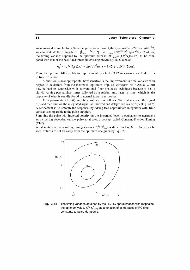
An approximation to h(t) may be constructed as follows. We first integrate the signalS(t) and then sum on the integrated signal an inverted and delayed replica of S(t) (Fig.3-12).A refinement is to smooth the response, by adding two approximate integrators with timeconstants comparable to the pulse duration.Summing the pulse with inverted polarity on the integrated level is equivalent to generate azero crossing dependent on the pulse total area, a concept called Constant-Fraction-Timing(CFT).A calculation of the resulting timing variance σt
2/ σt2(opt) is shown in Fig.3-13. As it can be
seen, values are not far away from the optimum one given by Eq.3.20.
Fig. 3-13 The timing variance obtained by the RC-RC approximation with respect tothe optimum value, σt
2/ σt2(opt), as a function of some ratios of RC time
constants to pulse duration τ.
10
10
1
1
0.1
0.1
RC / τ1
2RC / τ
1.05
1.6
2.5

3.2 Time-of-Flight Telemeters 5 9
3.2.4 Accuracy of the Sine-Wave Telemeter
Sine-wave modulation of power is a good strategy to impress time-localization infor-mation on a quasi continuous-wave source. It is especially used with semiconductor lasersthat are capable of supplying a substantial dc power and being modulated at high frequency,but are not good for pulsed operation at high peak power level.
Incidentally, the use of a modest power may even be a system requirement in applica-tions, like topography, that call for intrinsic compliance to laser-safety standards.To analyze the accuracy of the sine-wave telemeter, let us write the transmitted power as:
Ps (t) = Ps0 [1+m cos 2πfmt], (3.21)
where Ps0 is the mean transmitted power, fm is the modulation frequency, and m is the modu-lation index. The power signal returning from the target at a distance L=2cT is:
Pr (t) = Pr0 [1+m cos 2πfm(t-T)] (3.22)
In view of the system equation (Eq.3.5), the received mean power Pr0 is calculated fromPs0 as Pr0=Ps0GDr
2/4Leq2. The photodetected signal then follows as Ir (t)=σPr (t), with
σ being the spectral sensitivity of the photodetector, and is given by:
Ir (t) = Ir0 [1+m cos 2πfm(t-T)] (3.22’)
The distance to be measured is contained in the phase-shift ϕ=2πfmT of the receivedsignal relative to the transmitted one. An error ∆ϕ in phase reflects itself in a time error ∆T=∆ϕ/2πfm. By squaring and averaging, the relation between phase and time accuracy is:
σ2T = σ2
ϕ (1/2πfm)2 (3.23)
and, of course, the corresponding distance accuracy is σL =(c/2) σT.Now, contrary to the pulsed telemeter, we have a long measurement time Tr available
for averaging and a large number of sine-wave periods marking the time delay, not a singlepulse. Then, to implement the phase-shift measurement, we mix the received signal with areference local oscillator Ilo at the same frequency and with an adjustable phase, that is, witha signal of the form Ilo=I0 cos (2πfmt+ϕ0).Basically, the mixer is a circuit made of a square-law element and a time integrator to averagethe result, and it produces an output Sϕ= ⟨Ir Ilo⟩ of the two inputs Ir and Ilo applied to it. We may also regard the mixer as the circuit performing homodyne (electrical) detection of thesignal Ir (t), with the aid of a reference, the local oscillator Ilo. The result of the homodyningis a signal carrying the cosine of the phase difference.
Indeed, by inserting the expressions of Ir and Ilo in Sϕ= ⟨Ir Ilo⟩ and developing the co-sine product in sum and difference of the arguments, we get after some easy algebra:

6 0 Laser Telemeters Chapter 3
Sϕ = ⟨ I0 cos(2πfmt+ϕ0) Ir0 [1+m cos 2πfm(t-T)] ⟩ =
= (I0 Ir0 /2) m cos [2πfmT -ϕ0] (3.24)
The cos φ dependence in Eq.3.24 reveals that the mixer output is sensitive to the in-phasecomponent of the received signal, a well-known feature of homodyne detection. For φ≈0, thesensitivity of the mixer signal cos φ to small variations of φ is about zero. To have themaximum sensitivity, we shall work with signals in quadrature, and this can be done byadjusting the local oscillator phase to ϕ0=2πfmT+π/2.With this strategy, the mixer signal Sϕ is kept dynamically to zero, and the time measure-ment is obtained as T=(ϕ0+π/2)/2πfm.
We can write the total phase in Eq.3.24 as φ=π/2+ϕ to indicate that the mixer workson a small phase signal ϕ around the π/2 quadrature condition. The mixer output is thenSϕ=(I0 Ir0/2)m cos (π/2+ϕ) = -(I0 Ir0/2)m sinϕ ≈ -(I0 Ir0/2)mϕ for ϕ<<1.To take account of the fluctuation ∆Ir superposed to the received signal, we insert Ir+ ∆Ir inSϕ= ⟨Ir Ilo⟩ and change ϕ in ϕ+∆ϕ. Developing the product and averaging, we obtain Sϕ =(I0 Ir0/2)m sinϕ + ∆Ir (I0 /2) +(I0 Ir0/2)m∆ϕ .
From this expression, it is easy to find the relation between the phase vari-ance σϕ
2 =⟨∆ϕ2⟩, and received signal variance σ2
Ir =⟨∆Ir 2⟩ as:
σϕ2
= σIr2
/(m2Ir02) (3.25)
The corresponding relation, in terms of equivalent powers at the detector input (see Eqs.3.9and 3.10) is:
σϕ2
= pn2
/(m2Pr02) (3.25’)
Now, combining Eqs.3.25’ and 3.23 and using Eq.3.10, we obtain the time variance ofthe sine-wave modulated telemeter as:
σT2 = (1/2πfm)2 [(2hν/η) B (Pr0+ Pbg+ Pph0)]/(m2Pr0
2) (3.26)
As we can see from Eq.3.26, the primary dependence of accuracy in the sine-wave modulatedtelemeter is from 1/2πfm, the inverse of the angular frequency of modulation. By comparingwith Eq.3.16’, we see that 1/2πfm is the counterpart of the pulse duration τ in a pulsed te-lemeter. Further, in Eq.3.24 we can let B=1/2Tr for a measurement lasting a time Tr, and can intro-duce the number of received photons Nr= mPr0Tr contributing to the measurement. Withthese positions, we can rewrite Eq.3.24 as:
σT = (2πfm√Nr)-1 [(1/ηm) (Pbg+Pph0)/Pr]
1/2 (3.27)

3.2 Time-of-Flight Telemeters 6 1
As for the pulsed telemeter, the dependence of timing accuracy is from the inverse square rootof the total number Nr of signal photons collected in the measurement time Tr.
The counterpart of Eq.3.16’’, expressing the accuracy in terms of the equivalent photonnumber Nbg+ph0, is:
σT = (2πfm√Nr)-1 [(1/ηm) (Nbg+ph0)/Nr]
1/2 (3.27’)
By comparing the two equations, we can see that the performances are theoretically equiva-lent when we make 1/2πfm equal to τ and 2κS0/s’2 equal to 1/m.
Finally, let us consider the optimum filter treatment of the sine-wave modulated te-lemeter. If the signal waveform is given by Eq.3.22’, from Eq.3.18 the impulse response ofthe optimum filter is found as:
h(Tm-t) = sin 2πfmt /[1+m cos 2πfmt] (3.28)
At the measurement time Tm, the optimum filter weights the signal as s*h =∫0-Tm mcos 2πfmt × sin 2πfmt /[1+m cos 2πfmt] dt. For m<<1, the weight is sin 2πfmt, exactly thatof an in-quadrature homodyne detector.
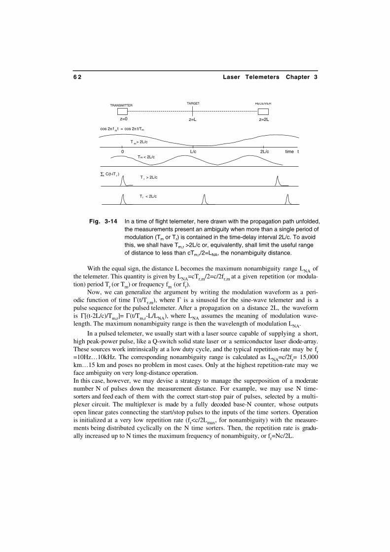
3.2.5 The Ambiguity Problem
In the preceding sections of this chapter, we have studied the theoretical performance oftime of flight telemeters and analyzed the dependence of accuracy from the physical parame-ters. This is the ultimate limit we can achieve in a well-designed telemeter and, as such, isthe first step of design before developing the details.
Now, we shall review the specific problems, if any, that originate from the measure-ment approach (the time of flight) we are considering. After doing so, we will be ready forthe instrumental development. Incidentally, this procedure has a general validity as a goodengineering approach to develop instrumentation.
A problem with time of flight telemeters is the measurement ambiguity arising be-cause the signal is inherently periodic (Fig.3-14).In the sine-wave modulated telemeter, ambiguity shows up when the period Tm=1/fm of themodulation waveform is shorter than the time of flight T=2L/c (and actually, we want asmall Tm to get a good accuracy). Thus, the phase-shift ϕ=2πfmT to be measured will be amultiple n2π of the round angle, plus a residual ϕ’, or ϕ= n2π+ϕ’. The phase meter meas-ures ϕ’ but cannot tell anything about n.In the pulsed telemeter, we get an ambiguity when the repetition time Tr is shorter than thetime of flight T=2L/c, and we send a second pulse before the first pulse has returned to thereceiver (Fig.3-14). Thus, for a pulse transmitted at t=0, we receive a correct return at t=T,but also spurious returns at t=T-Tr, T-2Tr, etc., due to the previous pulses still in flight.
A trivial cure to ambiguity is, of course, to keep Tr,m ≥T at all time. Using T=2L/c,the condition reads L≤cTr,m/2.
6 2 Laser Telemeters Chapter 3
Fig. 3-14 In a time of flight telemeter, here drawn with the propagation path unfolded,the measurements present an ambiguity when more than a single period ofmodulation (Tm or Tr) is contained in the time-delay interval 2L/c. To avoidthis, we shall have Tm,r >2L/c or, equivalently, shall limit the useful rangeof distance to less than cTm,r/2=LNA, the nonambiguity distance.
With the equal sign, the distance L becomes the maximum nonambiguity range LNA ofthe telemeter. This quantity is given by LNA=cTr,m/2=c/2fr,m at a given repetition (or modula-tion) period Tr (or Tm) or frequency fm (or fr).
Now, we can generalize the argument by writing the modulation waveform as a peri-odic function of time Γ(t/Tr,m), where Γ is a sinusoid for the sine-wave telemeter and is apulse sequence for the pulsed telemeter. After a propagation on a distance 2L, the waveformis Γ[(t-2L/c)/Tm,r]= Γ(t/Tm,r-L/LNA), where LNA assumes the meaning of modulation wave-length. The maximum nonambiguity range is then the wavelength of modulation LNA.
In a pulsed telemeter, we usually start with a laser source capable of supplying a short,high peak-power pulse, like a Q-switch solid state laser or a semiconductor laser diode-array.These sources work intrinsically at a low duty cycle, and the typical repetition-rate may be fr=10Hz…10kHz. The corresponding nonambiguity range is calculated as LNA=c/2fr= 15,000km…15 km and poses no problem in most cases. Only at the highest repetition-rate may weface ambiguity on very long-distance operation.In this case, however, we may devise a strategy to manage the superposition of a moderatenumber N of pulses down the measurement distance. For example, we may use N time-sorters and feed each of them with the correct start-stop pair of pulses, selected by a multi-plexer circuit. The multiplexer is made by a fully decoded base-N counter, whose outputsopen linear gates connecting the start/stop pulses to the inputs of the time sorters. Operationis initialized at a very low repetition rate (fr<c/2Lmax, for nonambiguity) with the measure-ments being distributed cyclically on the N time sorters. Then, the repetition rate is gradu-ally increased up to N times the maximum frequency of nonambiguity, or fr=Nc/2L.
TRANSMITTERRECEIVER
z=0
TARGET
z=L z=2L
time t2L/cL/c0
m
cos 2π f tm cos 2π t/Tm=
T > 2L/c
mT < 2L/c
rC(t-iT )T > 2L/cr
Σi
T < 2L/cr

3.2 Time-of-Flight Telemeters 6 3
This strategy is equivalent to expanding by a factor N the maximum nonambiguity range.In a sine-wave modulated telemeter, the ambiguity problem is more severe. Indeed, as
we work with a quasi-CW power, we cannot trade duty cycle for nonambiguity because re-ceived power and hence accuracy would be sacrificed.We can only use a modulation frequency fm low enough to avoid ambiguity on the distancerange to be covered. The nonambiguity range is LNA=c/2fm, and for LNA=0.15 km…1.5 kmwe need to keep the modulation-frequency fm as low as fm=1 MHz...100 kHz.
In contrast, both a semiconductor laser diode and the phase-measuring circuit can easilyhandle signals with modulation frequency up to several hundred MHz (that is, 3 decadehigher). Theoretically, the distance accuracy is σL=cσT≈c/2πfm√Nr from Eq.3.27, and the rela-tive accuracy is σL/LNA=1/π√Nr.Using Nr ≈107 detected photons, accuracy would be theoretically limited to ≈10-4 of themaximum range LNA, or we would get a measurement with no more than a four-decade dy-namic range.
In practice, the phase-measuring circuit may introduce an additional limit. The phaseresolution ∆ϕr is usually 10-3 or 10-2 of the round-angle 2π. Because the phase2π corresponds to LNA, the phase ∆ϕr corresponds to one unit of the least-significant digit inour measurement.This means that the dynamic range is limited to ≈1/∆ϕr, or only two to three decades in thisexample.To overcome this limit, we may take advantage that phase resolution does notworsen appreciably as the modulation frequency is increased up to the maximum that can behandled by the phase-measuring circuits.Because distance resolution is (c/2fm)∆ϕr/2π, we can then recover at least three decades ofdynamic range by working at increased frequency.
Of course, to exploit this possibility, we need to combine a high frequency of modula-tion for resolution and accuracy to a low frequency as required by the nonambiguity regime,which will be shown in the next sections.
3.2.6 Intrinsic Precision and Calibration
In a time of flight telemeter, we measure a time T and convert it to a distance L=cT/2.The intervening multiplication factor is the speed of light, c=299,793 km/s in vacuum [7]and c/n in a medium with index of refraction n.For propagation through the atmosphere, the most common case for a telemeter, n, differsfrom unity by a modest amount, yet about 300
.10-6 or 300 ppm (part-per-million).
Thus, as the time of flight measurement of distance comes to resolve the fourth or fifthdecimal digit, we have to care about the index of refraction of the air and apply the n-1 cor-rection to calibrate the instrument. In this way, we can have a calibration up to the fifthdecimal digit and eventually be able to reach the sixth.
The problem of air index of refraction correction is shared by interferometers, where wemay eventually go to the 7th or 8th decimal digit. Further information on the index of refrac-tion correction can be found in Sect.4.4.4.
6 4 Laser Telemeters Chapter 3
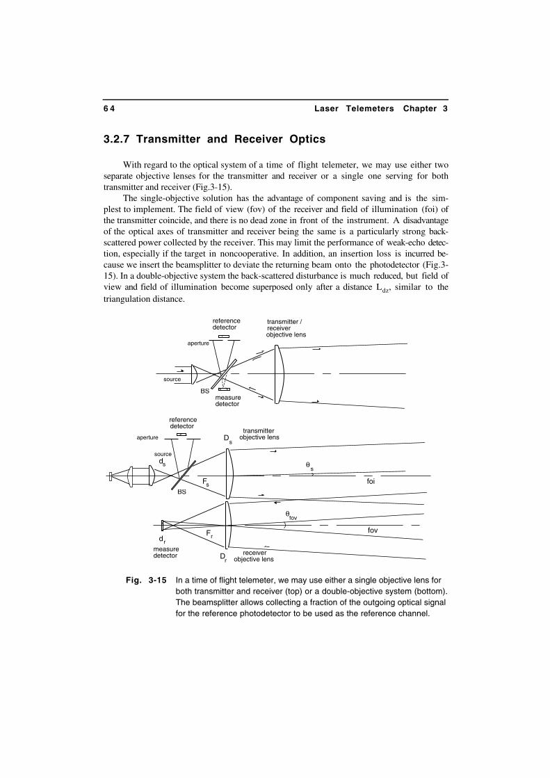
3.2.7 Transmitter and Receiver Optics
With regard to the optical system of a time of flight telemeter, we may use either twoseparate objective lenses for the transmitter and receiver or a single one serving for bothtransmitter and receiver (Fig.3-15).
The single-objective solution has the advantage of component saving and is the sim-plest to implement. The field of view (fov) of the receiver and field of illumination (foi) ofthe transmitter coincide, and there is no dead zone in front of the instrument. A disadvantageof the optical axes of transmitter and receiver being the same is a particularly strong back-scattered power collected by the receiver. This may limit the performance of weak-echo detec-tion, especially if the target in noncooperative. In addition, an insertion loss is incurred be-cause we insert the beamsplitter to deviate the returning beam onto the photodetector (Fig.3-15). In a double-objective system the back-scattered disturbance is much reduced, but field ofview and field of illumination become superposed only after a distance Ldz, similar to thetriangulation distance.
Fig. 3-15 In a time of flight telemeter, we may use either a single objective lens forboth transmitter and receiver (top) or a double-objective system (bottom).The beamsplitter allows collecting a fraction of the outgoing optical signalfor the reference photodetector to be used as the reference channel.
aperture
BS
sourceds
drmeasuredetector
sF
Fr
sD
rD
transmitterobjective lens
receiverobjective lens
sθ
fov
foi
referencedetector
BS
aperture
referencedetector
measuredetector
transmitter /receiverobjective lens
source
fovθ
3.2 Time-of-Flight Telemeters 6 5
Thus, unless provisions are taken to move the lens axes or the detector position at shortdistance, the measurement has a dead zone. A dead zone is, of course, a minor problem withlong-distance telemeters for geodesy, whereas it may be of importance in short-range teleme-ters intended for topography.
In both cases, a beamsplitter (BS in Fig.3-15) is inserted in the transmitter lens to pickup a minute fraction of the outgoing optical signal and to detect it by a reference-channelphotodetector. If the same type of photodetector is used in the reference and measurementchannels, errors due to residual phase-shifts or delays of them are canceled out.
The beamsplitter reflectivity at the surface hit by the outgoing beam is kept at 1% orless, whereas the other surface is either antireflection coated (double-objective case) or coatedto 50% reflection (single-objective case). In the double passage across the beamsplitter of theoutgoing and returned beams, the loss is TR=0.25 (or 6 dB) in the single-objective opticalsystem, as opposed to ≈ 0 dB in the double-objective system. If we take advantage that thelaser output is usually linearly polarized and add polarization-control elements to combinethe beams, the loss can be reduced to 3 dB. Last, we may go down to ≈0 dB if we replace thebeamsplitter with optical circulator, but the cost of this component is usually too high to beafforded. The zero-distance edge of the telemeter yardstick is determined by measurement andreference-channel photodetectors. Considering their virtual position along the transmitterpath, as produced by the beamsplitter, it is easy to see that the zero-distance location is themidpoint of the segment connecting these two positions.
Let us now consider the design of receiver and transmitter lenses. The constraint to startwith is the maximum allowable size of the objective lenses Dr and, of course, we want to beable to use the smallest detector size dr for the best noise and speed performance. To mini-mize dr, we need to keep the spot size wt on the target as small as possible.For a Gaussian beam, the minimum obtainable size as set by the diffraction limit is givenby wt =√(λL), where L is the target distance (see Sect. 1.1). Correspondingly, the transmitterobjective lens shall have a diameter Dt=(2wt)
1/2=(2λL)1/2 to project the spot wt at distance L.For L=100 m…10 km and at λ=1µm, we get Dt = 1.4…14 cm, which are quite reasonablevalues.
At the distance L, the spot wt is seen under the angle θfov = wt /L (=0.1…0.01 mrad inthe previous example). Working with a cooperative target (a corner cube), the retroreflectedbeam has a size 2wt at the receiver, and this value is the lens-size Dr we require.When the target is noncooperative (a diffuser), the received signal is proportional to Dr
2
(Eq.3.4) and we will use the largest Dr that is practically allowed by the application.To collect from a θfov field of view, we need a detector size dr >θfov Fr, where Fr is the focallength of the receiver objective. Letting Fr=100 mm, we get dr >10µm for θfov = 0.1mrad.
With respect to the transmitting objective, if the source collimated beam has a waistwl, we need a magnification M=wt /wl.Then, we set M=Ft /f, the ratio of the focal lengths of the two lenses constituting the colli-mating telescope indicated in Fig.3-15, top. If the source provides a near-field spot as anoutput (for example, is the output facet of a diode laser), we will use a separate collimatinglens to enter the telescope.This lens will include an anamorphic corrector to circularize the beam.

6 6 Laser Telemeters Chapter 3
3.3 INSTRUMENTAL DEVELOPMENTS OF TELEMETERS
In the following, we describe some conceptual approaches that have been used to de-velop pulsed and sine-wave modulated telemeters. As it is well known in instrumentation,the optimum design approach strongly depends on the available components and may be-come much different as the performance of components undergoes even minor changes. Atelemeter is no exception, and the examples reported in the following are illustrative of thedesign approaches and ingenuity of researchers in the last two decades.
3.3.1 Pulsed Telemeter
A very simple pulsed telemeter can be developed starting from the block schemeshown in Fig.3-16. Two objective lenses are used for the transmitter and receiver, and thestart pulse is derived with a beamsplitter from the outgoing optical beam. The stop pulse isdetected with the second objective lens aimed to the target.
Fig. 3-16 Block scheme of a pulsed telemeter using separate objective lenses fortransmitter and receiver. The start and stop pulses are used to gate onand off the counter, for which the input is a clock at frequency fc. After atime 2L/c, the counter content is then Ncount= fc2L/c, and this is the resultof a single measurement. With the aid of the buffer/adder, we may sumthe results of Nm successive measurement, getting a total Nm Ncount asthe output of the display. If the laser pulse response has a low time jitter,we may even use the driving signal of the pulser as a start pulse.
pulsed laser
start PD
pulser
stop PD
aperture
BS
COUNTERclock fc
c
start stop
target
buffer/adder display
out
fc
T
time sorters
control logicreset
enable
3.3.1 Pulsed Telemeter 6 7
If the light pulse is well correlated to the electrical drive of the laser, that is, the laserresponse to pulse drive has a low time jitter, we can also use the pulser signal itself as thestart pulse. This variant allows us to save a few parts (BS, PD, and preamp in Fig.3-16), andit can be used with semiconductor-diode sources, whereas crystal Q-switched lasers have anexcessive jitter.
Start and stop pulses enter time sorters to improve time localization and to standardizethe waveform for the subsequent input to the counter circuit. The counter is fed by a clock atfrequency fc, and the periods of fc are counted in the time interval T=2L/c defined by start andstop pulses. Thus, in a single measurement, the content of the counter we get is:
Ncount = fc T = fc 2L/c = L/(c/2fc) (3.29)
[In Eq.3.29, we implicitly assume to take the integer part of the quantities at the right handside of the equation]. Eq.3.29 tells us that the quantity c/2fc=L1 is the scale factor represent-ing the length of a single unit of Ncount, so that the mean value of distance L is:
L = Ncount L1 (3.30)
The quantity L1 also represents the unit U of rounding off in the measurement of L. Becausethe rounding-off error has a variance U2/12 and we make two truncation errors with the startand stop pulses sampling the clock, the total of the rounding-off error is twice as much, orU2/6. In terms of distance, this amounts to a variance σ2
L(ro)= L12/6.
Adding the timing error σ2t (Sect.3.2.3) multiplied by (c/2)2, we get the total distance vari-
ance of our telemeter as:
σ2L(tot, 1)= (c2σ2
t)/4 + L12/6 (3.31)
We may repeat the measurement Nm times to improve resolution and accuracy, providedthe application at hand allows for an increased total measurement time, now given by NmTrwhere Tr is the pulse repetition period. Repeating the measurement Nm times and summingup the results of each measurement, we get as an average of the accumulated counter content:
Ncount = Nm fc T = Nm L/(c/2fc) (3.29’)
Also, the distance variance decreases by a factor Nm, or:
σ2L(tot, Nm)= [c2σ2
t/4 +L12/6] /Nm (3.31’)
Now, we choose the clock frequency fc according to two criteria: (i) it shall have nu-merals such that Ncount represents the target distance L in metric units, and (ii) it shall behigh enough to attain the desired resolution.Because of requirement (i), we need L1=Nm c/2fc to be an exact decimal number, for example0.1, 1 or 10 m.

6 8 Laser Telemeters Chapter 3
As a first approximation, it is c=3.108 m/s, and hence the frequency should be fc=1.5.109, 1.5.108, and 1.5.107 Hz in the previous example for Nm=1.More precisely, if we take n=1.0003 and cvac= 299,793 km/s (see Sect.3.2.6), we have c=cvac /n=299,6731, and the numerals of fc are 1.4983655 (in place of 1.5). This value requiresa further correction against wavelength and temperature/pressure as we go to resolve the 5th-6th decimal digit (see Sect.3.2.6).Regarding the clock, we will use a good quartz-oscillator circuit, for which its accuracy infrequency may easily reach the 5th-6th decimal numeral, and even the 6th-7th in special units.
Because of requirement (ii), the order of magnitude of fc shall be compatible with theoptical pulse duration τ, and its value determines the required speed of the counter circuits.
As a rule of thumb, we should choose fc not much exceeding the inverse of the pulseduration 1/τ, so that the two terms in Eq.3.31’ contributing to the distance variance haveapproximately equal weights.Indeed, if we just take fc =1/τ, we have one count per pulse duration. This loosens the speedrequirement of circuits, but probably wastes some of the accuracy available in the pulsewaveform. On the other hand, taking fc =10/τ, we need faster circuits and better time sorters,but are able to optimize the time accuracy down to the limits discussed in Sect.3.2.3.
In general, when writing fc =M/τ where M=1..10 in the previous examples, the singlecount of the telemeter represents a length-equivalent increment c/2fc =cτ/2M.
To give a few examples, with a pulse duration τ=1, 10, 100 ns we have cτ/2= 0.15,1.5, 15 m, and L1=cτ/2M is a submultiple of these values, for example 0.05, 0.5, 5 m forM=3. Using fc =3/τ, the required clock frequency is fc = 3 GHz, 300 MHz, and 30 MHz re-spectively.
The case τ=30 ns, M=3, and fc =100MHz is representative of a pulsed-telemeter basedon a semiconductor laser source. Counters and sorters can work easily at this medium speed,and the circuits can be implemented at a relatively low cost. The least significant digit in asingle measurement of this hypothetical telemeter is 1.5 m.By repeating the measurement Nm (say 15…150) times, the resolution is increased by a fac-tor Nm and reaches 10… 1-cm, while accuracy improves by √Nm (=3.9...12). At a typicalpulse repetition rate fr=3 kHz, the total measurement lasts Nm /fr =5…50 ms.
The case τ =5 ns, M=7.5, and fc =1.5 GHz is representative of a pulsed telemeter basedon a Q-switched solid state laser. The least significant digit is now 0.1 m in a single meas-urement, a figure already adequate for applications requiring a good accuracy and a single-shotmeasurement time.
Typical applications calling for the previously mentioned specifications are (i) altime-ters for helicopters; (ii) terrain profilers, like the MOLA telemeter mission (Fig.1-5, see [8]);(iii) satellites ranging observatories (see [9] as an example); (iv) military telemeters and (v)long-distance geodesy [10].
In all these applications, as we go to long distances, we have to increase the peakpower of the pulse and the collecting aperture of the receiver by using a large-aperture tele-scope.
Then, it is advisable to use just one optical element for both transmitter and receiver,as shown in Fig.3-15 (top).

3.3.1 Pulsed Telemeter 6 9
In this configuration, a beamsplitter inserted in the outgoing optical path collects a fractionof the optical pulse for use as the start signal.
Several different approaches for pulsed telemeters have been proposed in the scientificliterature, and an interesting selection of papers on the subject is provided by Ref.[1]. Moreresults were presented recently at specialized conferences [11].
3.3.1.1 Improvement to the basic pulsed setup
By slightly modifying the time interval measurement described in the previous sec-tion, we can get rid of the start/stop rounding-off error and improve the distance variancedown to the ultimate limit of pulse-timing variance σ2
t.The idea consists of combining the coarse measurement of time interval, performed by
clock counting, with a fine measurement of the fraction-of-period excess ∆Tex in both startand stop pulses.
As illustrated in Fig.3-17 for the start pulse, we can recover this fraction ∆Tex by us-ing the discriminator output to trigger the start of a Time-to-Amplitude Converter (TAC).
Fig. 3-17 The fraction-of-period time interval ∆Tex between start pulse SP and thefirst counted clock pulse (CP1) that can be recovered by this circuit toimprove accuracy of the telemeter. The scheme is duplicated for the stoppulse.
stretcher output
threshold
start/stop, photodetected pulse (SP)
time
clock pulses C
time
time
output from time-to-amplitude converter
photodetected pulse, SP
threshold crossing discriminator
clock pulses
threshold crossing discriminator
time-to-amplitude converter (TAC)
start
stop
stretcher
ADC
discriminator output
CP1
∆Tex

7 0 Laser Telemeters Chapter 3
The stop to the TAC is provided by the first clock pulse arriving after the discriminatorswitch-on. Using a stretcher to increase the duration of the discriminator output, in combina-tion with an AND gate receiving the clock pulse, we can sort out this first clock pulse (CP1in Fig.3-17). Then, the amplitude of the output from the TAC is proportional to the required time ∆Tex.By converting the TAC signal amplitude to a digital output with the aid of an Analog-to-Digital Converter (ADC) we get ∆Tex (and the corresponding L1) digitized in, say, one ortwo decades. Of course, the same procedure will be used for the stop pulse to recover thefraction of period excess of it and to correct the result accordingly.
Note that the two more discriminations in Fig.3-17, performed on the clock pulses, donot appreciably degrade the accuracy. In fact, like the start (photodetected) pulse, clock pulsesare large in amplitude, and their time variance σ2
t is negligible [from Eq.3.16] as comparedwith the σ2
t of the stop (photodetected) pulse.
3.3.1.2 Pulsed telemeters using slow pulses
Two techniques can be used to improve resolution down to nanoseconds when thepulse available from the laser source is rather slow, for example, microsecond-long as forCO2 laser sources. They are the vernier technique and the pulse-compression technique dis-cussed below.
Vernier Technique. This is a technique well known in nuclear electronics [12] to in-crease time resolution in measurements with slow waveforms.As shown in Fig.3-18, the optical start and stop pulses are detected by a photodiode, a nearlyideal current generator. The currents excite two resonant, parallel LC-circuits. The LC cir-cuits are designed to have a high Q-factor, and the voltage VLC across them is taken throughhigh impedance to preserve the initial Q.With a reasonably high Q, the voltage VLC is a nearly sinusoidal oscillation, and it dampsout slowly after excitation, making many periods of oscillation (N≈πQ) available for themeasurement.
Timing is performed by looking at the zero-crossing of the VLC waveform. Indeed, VLCstarts oscillating after the pulse has ended and its charge has been completely collected by thecapacitor. It can be shown that VLC carries the timing information associated with the centerof mass (or time-centroid) of the pulse, provided the pulse duration is short as compared withthe oscillation period.
Now, let us compare the start and stop waveforms VLC1 and VLC2 (Fig.3-18). The timedifference between the start and stop centroids (or, between the negative-going zero-crossingsof VLC1 and VLC2) can be written as T=T0+∆T. Here, T0 is the coarse delay between theVLC1 and VLC2 oscillations and is given by an integer multiple of the resonant period 1/f0,whereas ∆T is a fine delay, given by a fraction of 1/f0 (Fig.3-18).
The coarse measurement is readily obtained by counting the number of periods Nc,which are contained in VLC1 after its first zero-crossing and before VLC2 makes its own firstzero-crossing.

3.3.1 Pulsed Telemeter 7 1
To get the fine measurement, the resonant frequencies of the start and stop circuits aremade slightly different, let us say f0 (start) and f0/(1-∆) (stop).Then, signal VLC1 initially leads VLC2, but suffers a small delay, with respect to VLC2 at eachperiod. The small delay is 1/f0 -(1-∆)/f0 = ∆/f0. After a number Nf of periods has elapsed,the stop waveform VLC2 finally leads the start waveform VLC1.
Fig. 3-18 The vernier technique uses two resonant circuits fed by the start and stopphotodiodes to perform the time delay measurement. It resolves a smallfraction of the resonant period, even with relatively slow (low-noise, how-ever) optical pulses. The resonant circuits have a slight offset in resonantfrequency. The coarse measurement of time delay is made by counting thenumber of periods of the start oscillation before the stop is received (timeT0). The fine (or vernier) measurement of the fraction of period ∆T is made bycounting the number of periods contained in the start oscillation before thestart oscillation, initially in delay, becomes in the lead (see Fig.3-19 for theelectronic block scheme).
PULSED LASER1µs duration,10 kHz rep rate
tP
Pr
VLC2
LC1V
0T ∆T
≈1µs >100µs (15 km)
START
STOP
2
response of startresonant circuit
C L
LC1V
start PD
stop PD
C L
VLC2
resonant circuit at f =150kHz1 2
resonant circuit
at f =150/(1-∆ ) kHz
∆ = 0.005
1
response of stop resonant circuit
a number of periodselapses before stopresponse leads start

7 2 Laser Telemetry Chapter 3
Counting the number Nf of periods we find in VLC1 after VLC2 has done its first zero-crossing,until VLC2 leads VLC1, we get the measurement of ∆T in units of ∆/f0.
Example. With a τ=1-µs pulse (for which the resolution is cτ/2=150m), we may choose f0=150 kHzas the resonant frequency of the LC circuits. The period 1/f0 corresponds to a distance incrementc/2f0 =1000 m and is the least significant digit of the coarse measurement. In addition, by taking∆=0.005 as the resonance offset, we resolve ∆c/2f0 =5 m. This is the least significant digit of thefine measurement. The maximum number of periods 1/f0 we have to count in the vernier operation i s1/∆ =200 and, therefore, we need a Q factor of about 200 to keep damping of VLC waveforms rea-sonably low. Of course, the τ∆= 5ns resolution will be actually obtained if the received pulse car-ries an adequately large number of photons (Eq.3.16).
Fig. 3-19 Electronic processing of signals from the vernier telemeter of Fig.3-18 canbe made with a variety of approaches. The one shown here is perhaps theeasiest to implement. Resonant signals are buffered and passed though adiscriminator. By time differentiation, we get positive and negative pulsesmarking the periods. A logic circuit (middle flip-flop and AND gate) countsthe negative transitions of VLC1 until VLC2 makes the first negative-goingoscillation. These counts go to the 1 and 10-km decades. The verniermeasurement is made by the top flip-flop and AND gate. Here, we countthe positive transitions of VLC1 until the negative-going VLC2 leads thenegative-going VLC1. This gives the two-and-a-half decades with resolu-tion down to 5m.
LC1V
VLC2
buffer anddiscriminator
time differentiator
1
0
decadecounter
buffer anddiscriminator
time differentiator
polaritysorter
+
-
polaritysorter
+-
set
reset
timeout clock
decadecounter
AND
1
0
1
0
decadecounter
decadecounter
count
AND
reset to allflip-flops
5 m10 m100 m1 km10 km

3.3 Instrumental Developments of Telemeters 7 3
The centroid-timing corresponds to weighting the pulse waveform by t-t0. This is actu-ally the operation performed by the optimum filter when the received pulse has a Gaussianwaveform (see Sect.3.2.3.1). Because the Gaussian is a very popular approximation, we mayconclude that the LC timing and vernier technique are near-to-optimal choices in most practi-cal cases.
Pulse-Compression Technique. This technique has been demonstrated with a CO2 lasersince the early times of laser telemeters [13] as an adaptation to optical frequency of a well-known method used in the microwave radar.
As shown in Fig.3-20, we may start with a Continuous Working (CW) source, such asone like the CO2 laser that may be difficult to pulse, but that makes a large power available,e.g., a few Watts.
Fig. 3-20 With the pulse compression technique, we can transmit slow (µs) opticalpulses and shorten them after photodetection to a width adequate for con-ventional timing. Compression is achieved by a scheme similar to that usedin radar techniques, which involves chirped modulation and demodulation.
CW laser(CO2, 3W)
LiNbO3 A-OMODULATOR
CMT (HgCdTe)IR photodetector
preampl
SAW
chirpgenerator
SAW pulsecompressorU' U
0 4 µs 30 µs
U
U, P
P
U'
rectified signalfor conventionaltiming
100 ns
time
time
time
≈240 periods@ ≈60 MHz
compressed signal≈ 6 periods

7 4 Laser Telemetry Chapter 3
A reason to use a CO2 laser source is that the Far-Infrared (FIR) wavelength of emis-sion, λ=10.6µm, is favorable for a much larger range of operation in turbid media, such asfog and smokes (see App.A3.1 and Fig.A3-7). The relatively large CW power is readily pro-vided even by compact CO2 sources and is desirable to compensate for the decreased detectorsensitivity and increased propagation attenuation.
Using an acousto-optics modulator [14], we are able to impress a modulation on the av-erage power in form of sine-wave bursts, as indicated in Fig.3-20.
The repetition period Tb of the burst is dictated by the desired ambiguity range(Sect.3.2.5), and a typical choice for an airborne telemeter is Tb=30 µs (La=4.5 km). A burstduration τb which is relatively short for timing purposes, but long enough to accommodatethe chirp modulation, is the value τb=4µs shown in Fig.3.20.
With a CO2 laser, these times are short as compared with the active-level lifetime(τ21≈400µs), and therefore the average power is the same as the CW value PCW. Then, thepeak power of the burst is Pp=PCW/η, or, it is increased by the inverse of the duty cycleη=τb/Tb (a factor of 7.5).
For the pulse compression, we shape the burst waveform as a chirped sinusoid, or a lin-ear-sweep frequency modulation ranging from f0 at the beginning of the burst to f0+∆f at theend of the burst. Such a chirped sinusoid can be synthesized by a number of circuits, yet theSurface Acoustic Wave (SAW) is the most neat and simple to implement [14]. Typical valuescompatible with the performance of the lithium-niobate modulator are f0=60 MHz and ∆f =10MHz. Thus, we have ≈60MHz×4µs=240 periods of sinusoidal oscillation in the burst, withan instantaneous frequency increasing from 60 to 70 MHz.
The chirp is a sort of (frequency) dispersion of the impulse response of the circuit gener-ating the modulating wave. We may cancel it by cascading, after detection, a second chirp-generating circuit with the same dispersion, but opposite sign. The circuit shall have a reso-nant response lasting the same time τb, but with f0+∆f at the beginning and f0 at the end ofthe burst. With a SAW device, this is particularly easy because we need only to interchangeinput and output of the device.Theoretically, the compression ratio is found as τb∆f [13]. With the previously chosen val-ues, it is a factor 10MHz×4µs=40, and then the compressed duration is 4µs/40=100ns, andrise/fall times may be ≈1/60MHz≈15ns.In the compression, we gain an increase of (equivalent) peak power of τb∆f. In addition, afactor 1/η=Tb/τb comes from the repetition rate. Thus, the total increase respect to the CWvalue is factor (Tb/τb)(τb∆f)=Tb ∆f =300, a remarkably good value indeed.
After rectification of the compressed envelope, we may proceed in the timing operationby conventional processing of signals.
3.3.2 Sine-Wave Telemeter
The sine wave telemeter allows using a low-power laser, provided it can be modulated at rea-sonably high frequency. Indeed, the theoretical accuracy of the sine-wave telemeter equals thatof the pulsed telemeter when the inverse angular frequency 1/2πfm of modulation is equal tothe pulse duration τ (Sect.3.2.4), and we use the same number of collected photons.

3.3 Instrumental Developments of Telemeters 7 5
Low power is desirable and may even be a mandatory requisite in view of laser safety is-sues (App.A1.5). This is especially true for outdoor applications in the presence of the pub-lic, for example the topographic telemeter replacing the theodolite, the laser level and align-ment equipment. In such applications, either we use barriers to prevent exposure of humansto a hazardous level, or work with the maximum power allowed by a Class-1 laser.For semiconductor laser diode operating at a wavelength λ=700-900 nm, this power is Pt =0.2-0.6 mW, a reasonable value readily provided by ternary GaAlAs lasers. These lasers are cheap,reliable, and compact, and can be easily modulated through the injected current up to severalhundreds MHz.
The problem of ambiguity (Sect.3.2.5) has been approached by a number of methods[1,11], and in the following we describe two of them, perhaps the most practicable becausethey have been incorporated in products. They are the frequency-sweep method and the multi-frequency method.
Frequency-sweep method. We use a sinusoidal waveform for modulating the laser powerand vary the modulation frequency fm in time. We start with a frequency fm0 low enough toensure the desired non-ambiguity distance LNA and sweep it up to a large value fM0 that allowsus to reach the desired distance resolution ∆L, as indicated in Fig.3-21.
Fig. 3-21 In a sine-wave modulated telemeter, we want to avoid the distance ambigu-ity and yet be able to use a high-modulation frequency. To this end, fre-quency is made to sweep from a very low value fm0 (typically 15 kHz, avoid-ing ambiguity up to 15 km) to a fairly high fM0 (typically 150 MHz, adequatefor a 1-cm resolution). The coarse measurement is recovered from the num-ber of zero-crossings contained in the phase signal Sϕ, while frequency issweeping from fm0 to fM0.
m0f
M0f
fm
0 Ts Tr
+π
-π
0
S (t)ϕ
time
time
S (t) makes N=L/[c/2f ]ϕ M0
zeroes (or 2π ) crossings (coarse measurement)
is the phase in excess of 2 πN (fine measurement)ϕ sS (T )
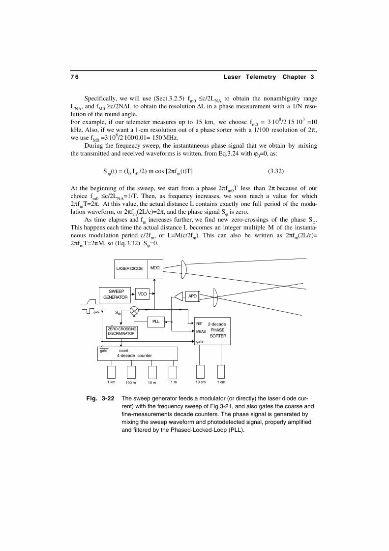
7 6 Laser Telemetry Chapter 3
Specifically, we will use (Sect.3.2.5) fm0 ≤c/2LNA to obtain the nonambiguity rangeLNA, and fM0 ≥c/2N∆L to obtain the resolution ∆L in a phase measurement with a 1/N reso-lution of the round angle.For example, if our telemeter measures up to 15 km, we choose fm0 = 3.108/2.15.103 =10kHz. Also, if we want a 1-cm resolution out of a phase sorter with a 1/100 resolution of 2π,we use fM0 =3.108/2.100.0.01= 150 MHz.
During the frequency sweep, the instantaneous phase signal that we obtain by mixingthe transmitted and received waveforms is written, from Eq.3.24 with ϕ0=0, as:
S ϕ(t) = (I0 Ir0 /2) m cos [2πfm(t)T] (3.32)
At the beginning of the sweep, we start from a phase 2πfm0T less than 2π because of ourchoice fm0 ≤c/2LNA=1/T. Then, as frequency increases, we soon reach a value for which2πfmT=2π. At this value, the actual distance L contains exactly one full period of the modu-lation waveform, or 2πfm(2L/c)=2π, and the phase signal Sϕ is zero.
As time elapses and fm increases further, we find new zero-crossings of the phase Sϕ.This happens each time the actual distance L becomes an integer multiple M of the instanta-neous modulation period c/2fm, or L=M(c/2fm). This can also be written as 2πfm(2L/c)=2πfmT=2πΜ, so (Eq.3.32) Sϕ=0.
Fig. 3-22 The sweep generator feeds a modulator (or directly) the laser diode cur-rent) with the frequency sweep of Fig.3-21, and also gates the coarse andfine-measurements decade counters. The phase signal is generated bymixing the sweep waveform and photodetected signal, properly amplifiedand filtered by the Phased-Locked-Loop (PLL).
LASER DIODE MOD
APDVCO SWEEP GENERATOR
gate
PLL
count4-decade counter
gate
100 m 10 m 1 m
2-decade PHASE SORTER
gate
10 cm 1 cm1 km
SϕZERO CROSSING DISCRIMINATOR
REF
MEAS
ΦS

3.3 Instrumental Developments of Telemeters 7 7
When the sweep finally reaches its maximum frequency fM0, the number of zero-crossings that the phase signal Sϕ has done is exactly the number of times M0 the distancec/2fM0 is contained in the distance L to be measured.
We may count the zero-crossings of Sϕ by using the (positive) slope of the sweep sig-nal as a gate input to a 3-decade counter (Fig.3-22). In this way, we obtain the coarse meas-urement of distance in units of c/2fM0 (=3.108/2.150 MHz = 1 m).
In the schematic of Fig.3-22, this processing is done by mixing the signal of the modu-lator and the signal received from the photodetector. Actually, the signal from the photodetec-tor may be noisy and, to filter it, a Phase-Locked-Loop (PLL) block is used.
The PLL is equivalent to a narrow pass-band filter with the central frequency dynami-cally tracked to the signal frequency. A narrow bandwidth is desirable to effectively filter outnoise from the phase signal, to avoid counting spurious zero-crossings. The smallest band-width we can use in the PLL filter is determined by the sweep duration Ts as B≈1/Ts.
Fig. 3-23 Simplified block scheme of a typical 2-decade phase meter. The measure-ment is performed at an intermediate frequency (1kHz), that is tied througha :100 divider to a main oscillator (100 kHz), which is also used as a clock ofthe counter. The MEAS signal is down-converted to 1kHz by mixing with theREF signal shifted by 1kHz. Start and stop to the counter are obtained byzero-crossing discrimination of the MEAS and REF signals.
gate
MEAS
SϕZERO-CROSSING DISCRIMINATOR
SϕZERO CROSSING DISCRIMINATOR
start
stop
clock periods counted
start
stop
INTERMEDIATE FREQUENCY OSCILLATOR (1 kHz typ)
1 kHz
REF(f )m
MEAS
REF 1 kHz
CLOCK@100 kHz
/100 DIVIDER
count
2-DECADE
BCD COUNTER
OUTPUT BUFFER
m(f )
7 8 Laser Telemetry Chapter 3
The fine measurement is performed on the phase-signal Sϕ during the period from Ts toTr (Fig.3-21) when the modulation-frequency is kept constant (fm= fM0). A conventional 2-decade digital phase meter is adequate to sort out the measurement (Fig.3-22).
As detailed in Fig.3-23, a typical design uses a conversion of the signal (MEAS) to anintermediate frequency, usually fIF=1 kHz. The periods of a clock running at fck=NfIF (100kHz for N=100) are counted using REF and MEAS signals as start and stop.
Fig.1-4 is an illustration of a commercial sine-wave modulated telemeter developed onthe frequency-sweep concept for the application in topography. The resolution of such a te-lemeter may be 1 cm (for a 10-s measurement time). Distance of operation can go up to 100to 300 m when using a cooperative target. Usually, the target is a corner-cube array with ≈50to 200 cm2 area. The optical source is typically a 0.1 mW GaAlAs laser, and the entire in-strument, including the electronic processing unit, fits in a briefcase for use in the field.
Multifrequency method. Another approach to the sine-wave telemeter is using a fre-quency fm1 low enough to avoid distance ambiguity, together with its multiples, 10fm1,100fm1, etc., to achieve the desired resolution. The ingenuity is in properly combining themeasurements performed by the different frequencies.For example, if we choose three frequencies that are a multiple of a factor 100 and use a 1/100round-angle phase measurement, each frequency supplies two decades, and as a whole we cover3×2= 6 decades in distance.
As shown in Fig.3-24, the three measurements can be made in sequence by multiplex-ing the modulation waveforms to the laser and distributing the results to the appropriatecounters.To substantiate the concept, let us take fm1=15 MHz as the highest frequency. The correspond-ing distance is Lm1=c/2fm1=10 m, and the 10-cm and 1-m digits come out from the 2π/100phase measurement.Then, the second frequency will be fm2 =150 kHz to supply the 10-m and the 100-m digits,and the third frequency fm3 =1.5 kHz, gives the 1-km and the 10-km digits.
Theoretically, the measurement associated to each frequency is the pair of digits in Lremaining from the next lower frequency. In fact, from Eq.3.24, the phase argument of thecosine, the quantity to be measured in 2π/100 intervals, can be written as:
ϕm1 = 2πfm12L/c = 2π L/Lm1
where Lm1 is the scale factor associated to fm1. As the phase is modulo 2π, we measure theremainder of L/Lm1 from the integer part, or the first two decimals. Considering thatfm2=fm1/102
and fm3=fm1/104, we have ϕm2=2π102L/Lm1 and ϕm3=2π104L/Lm1.Thus, the measurements with fm2 and fm3 are the remainders of 102L/Lm1 and 104L/Lm1 fromthe integer part, or the second two decimals and the third two decimals, respectively, ofL/Lm1.
A subtle problem arises, however. We may even tie the three frequencies very precisely,i.e., deriving them from a single oscillator through dividers, but unavoidably measurementerrors will prevent the results from being exact multiples of each other.

3.3 Instrumental Developments of Telemeters 7 9
Thus, when the 10-cm and the 1-m digits pass from 99 to 00 (or vice-versa), the digit of the10-m does not increment (or decrements) the content by one. Instead, the 10-m digit mayswitch erratically, when the 10-cm and the 1-m digits are somewhere, e.g., between 90 and 10(as they pass through 99 and 00).This problem is clearly a very basic one, common to all readouts from demultiplied scales andcalls for a technique of digital synchronization.
Fig. 3-24 The multifrequency method of the sine-wave modulated telemeter uses threefrequencies, multiples of 100, to obtain a large nonambiguity range with thesmallest of them (fm3≈1.5kHz), yet has a good resolution with the largestavailable (fm1≈15MHz). To try balancing the electronic delays, the REF signalis obtained by a photodetector and amplifier combination identical to that of theMEAS for the pulse returning from the target. The 1-KHz local oscillator shiftsall three frequencies so that, after mixing with REF and MEAS, the phasemeasurement is always performed at the same intermediate frequency. A logiccircuit provides synchronization of the three pairs of digits.
100 m 10 m 1 m 10 cm 1 cm1 km
APD
LASER DIODE MOD
OSCILLATOR, 15 MHz
:100
:100
SCALER
SCALER
f
f
f
APD
REFERENCE CHANNEL
MEASUREMENT CHANNEL
INTERMEDIATE FREQUENCY OSCILLATOR (1 kHz typ) 2π/200 phase measurement
1:3 buffer multiplexer
T clock
T clock
T clock
m1
m2
m3
MEASREF
logic synchronizer

8 0 Laser Telemetry Chapter 3
To synchronize the digits, we add a redundancy to the coding scheme. Instead of the2π/100 resolution for the ×100 frequency ratio, we double the resolution to 2π/200 in fm2 andfm3.In this way, we can make available a logic variable, say it X1/2, which indicates the state (00to 49 or 50 to 99) of fm2. Nominally, X1/2 replicates the most significant bit of the fm1 read-out, let us say it Y50. This bit Y50 changes from 0 to 1 and from 1 to 0 when the digits offm1 go from 00 to 49 and from 50 to 99, respectively. Because of measurement errors, X1/2deviates from Y50, however.
By comparing the two variables, it is easy to determine if the fm2 (and fm3) bit shall beincremented by one or not. Thus, synchronization is obtained at the expense of a modest lossin resolution (a factor of 2).The multifrequency technique is incorporated in commercially available telemeters, and ityields performance comparable to those of frequency-sweep, sine-wave modulated telemeter.
3.4 IMAGING TELEMETERS
A number of applications, ranging from military to biomedical, call for a spatially re-solved measurement of distance, or imaging telemeters. When single-point telemeters reacheda technical maturity in the 1990s, research started to deal with the extension of the measure-ment on a two-dimensional (2-D) array of points (or pixels).
Reason for interest in image telemetry, also called imaging laser radar and three-dimensional (3-D) imaging, stems from the benefit that distance information adds to the im-age morphology.
In a parallel but separate branch of technical evolution, multispectral imaging has alsomatured in the years. This is a segment offering a variety of information about the detailscontained in a scene, viewed at visible (λ=0.4-0.7 µm) as well as at near infrared (λ =0.8-2 µm) and far infrared (λ =3-12 µm) wavelengths.
Adding the distance information to imaging systems greatly helps solve the problem ofAutomatic Target Recognition (ATR), both in the military and robotic segments of applica-tion [15].
Of course, an imaging telemeter can be developed by combining a normal single-pointtelemeter and a 2-D scanner device that aims, in a raster or TV-like format, to each pixel ofthe scene in an ordered sequence. We need also an optical switch in the path outward from thelaser, because we shall turn off the beam when the scanner reaches the end of a line and thebeam shall flyback to the beginning of the next line. As a scanner, we may use a pair of Xand Y mirrors, mounted on galvanometer actuators.
This solution enables us to form an image with typically N=100×100 pixel, a 5°×5°angular field of view, and a reasonable frame repetition rate (10 to 30 frames per second).The switch could either be an electro-optical cell (KDP or LiNbO3 crystals), or an acousto-optical switch (LiNbO3 or CdTe). Both switches are fast enough (settling time of microsec-onds) to match the speed required by galvanometer-scan systems. Wavelength of operation ofthe imaging telemeter can go, depending on the application, from the visible, using diode
3.5 The LIDAR 8 1
lasers, to the near and far infrared. The benefit of far infrared wavelengths is the mitigation ofscattering attenuation and turbulence effects (Ref.[15] and App.A-3), both in a normal atmos-phere and in light fogs and hazes. A few imaging laser radars operating at several wave-lengths, from 1.0 to 10 µm, have been evaluated in [15] in good and low visibility condi-tions.
Because the measurement time is subdivided between N pixels, the theoretical accuracyof the imaging telemeter is worse than that of a still staring telemeter by a factor √N (≈100in the previous example). However, this is not a severe hindrance from the practical point ofview. It turns out that the extra information gathered from the frame-size image largely allevi-ates the resolution or precision requirement as compared with the single-point measurement.
About the measurement configuration, imaging telemeters were first demonstrated withpulsed laser sources [15], so they were time-of-flight pulsed telemeters. The sine-wave con-figuration has been recently used as well [16] in connection to a 3-D imaging application.The advantage of sine-wave modulation is that we can use an image detector and retrieve thedesired phase from each pixel without scanning the scene.In the experiment [16], a wide-angle laser beam from a 900-mW LED source illuminates a64×25-pixel scene. The source is amplitude-modulated at 20 MHz, and the measurement islimited to the nonambiguity distance Lna=7.5 m. A CCD array (Ref.[2], Sect.9.2) receives thelight diffused by the scene through an objective lens conjugating each scene pixel to a pixelin the CCD. In the CCD, the electrode commanding the storage of the photogenerated chargeis driven by the modulating waveform at 20 MHz.The efficiency of charge collection depends on the voltage on the storage electrode, so theuseful CCD output current is the product of the received radiant power and of the modulatingwaveform, or the phase φ=2ks. The phase is read with <10-3 resolution resulting in a distanceerror of a few cm.
3.5 THE LIDAR
Actually not a telemeter, but similar to it (see Fig.1-6), the LIDAR (acronym for LaserIdentification Detection and Ranging) is an instrument for the remote sensing of the naturalmedia (mainly the atmosphere, but also water masses). In particular, the LIDAR is routinelyused to probe pollutants of the atmosphere and to obtain distance-resolved maps of them forambient protection (Fig.1-6). The LIDAR has also been successfully used in a number ofscientific surveys, including ozone and vertical temperature profile in Antarctica, plankton andchlorophyll on the sea surface, etc. [17-20].
In a LIDAR, we use a pulsed source with high peak power, usually a Q-switched laser,and choose the wavelength in correspondence to an absorption peak of the atmospheric com-ponent to be measured. The wavelength range of interest spans from the near-UV (300 nm) tothe far IR (10 µm) as opposed to millimeter and centimeter wavelength employed by a mi-crowave radar. Plenty of useful lines are found at optical wavelengths [17], virtually for anykind of gaseous species we can find in the atmosphere. These include, for example nitrogen,oxygen, and carbon oxides; water vapor, ozone, and dangerous species like sulphur oxides, hy-

8 2 Laser Telemetry Chapter 3
drocarbons, fuel gases, chlorofluorocarbons (CFCs), etc. From one side, the abundance of lines means that hardly a species will be found that
cannot be measured in the optical range by a LIDAR technique. On the other hand, the crowd-ing of many lines pertaining to different species will make it hard to distinguish between dif-ferent constituents. Thus, the LIDAR will make measurements and actually work with unpar-alleled sensitivity on constituents known to be present in the medium under test, whereas thediscrimination between similar species will be poor, in general. With regard to the sensitiv-ity, the actual figures will depend on parameters like species, measurement technique, powersource, and wavelength range. The typical sensitivity, expressed as the minimum detectableconcentration per unit volume, may range from 10 ppb×m (part per billion, or 10-9, per meterof propagation path) to perhaps 10 ppm×m (part per million per meter).
To tune the wavelength on a wide spectral range and cover most species of interest, thelaser may be an Optical Parametric Oscillator (OPO) [21]. The OPO is pumped by a Q-switched laser at fixed λ, like Nd:YAG at 1.06µm or at 0.53µm with second harmonic gen-eration (SHG), and can be tuned from about 0.6 to 3.5µm. Other options for tunable sourcesin the visible and near-infrared are the alexandrite laser (0.8-0.9µm) and several dye lasers (0.4to 1.0µm) [22]. For the infrared, CO2 and CO lasers have been widely used, as well as lead-salt semiconductor diodes.
The optical beam is collimated by the transmitting telescope and sent through the at-mosphere along the line of sight. There is no need to place a distant target, except for safetyissues. Line of sights of successive pulses are arranged in a raster sequence so that a map ofmeasurement can be constructed. For each pulse, power back-scattered by the atmosphere iscollected back by the receiving telescope and is converted into an electrical signal by the pho-todetector. The time dependence of the photodetector signal is easily translated into a distancedependence of the back-scattering strength.
To calculate the signal received by the LIDAR, we start assuming that the transmittedpulse is very short and write it as P(t)=Eδ(t), where δ is the Dirac-impulse function and E isthe energy contained in the pulse. Upon propagation to a distance z=ct, the optical signal isdelayed and attenuated, and it can be written as:
P(t) = E δ(t-z/c) exp -∫α dz
Here, z/c is the time delay, and α=α(z) is the attenuation coefficient of the atmosphere. Theback-scattered power going toward the source in the interval z⎯z+dz is then:
dP(t) = E δ(t-z/c) [ exp -∫αdz ] f(θ) α dz dΩ
In this expression, θ and dΩ are the scattering angle and the solid angle of collection, respec-tively, and f(θ) is the scattering function (see Appendix A3-1 and Fig.A3-5).
By integrating dΩ around θ=180°, the direction along which we collect the back-scattered radiation, we get ∆Ω=πD2/4z2 as the total solid angle subtended by the receivinglens of diameter D. Letting σbs(z)= f(180°)α for the back-scattering coefficient, and also con-sidering the delay and the attenuation experienced in the backward propagation, the back-scattered power collected at the receiver is obtained as:

3.5 The LIDAR 8 3
dPbs(t) = E σbs(z) (πD2/4z2) δ(t-2z/c) [exp-2∫αdz] dz (3.33)
From Eq.3.33 we can see that, by launching a short δ-like pulse at time t=0, we receiveat time t=2z/c an elemental power contribution dPbs(t) in an elemental time dt=dz/c. The in-tensity dPbs(t)/dt is proportional to the back-scattering of the atmosphere σbs(z), to the expo-nential attenuation exp -2 ∫ αdz, and to a distance-dependent term (D/z)2.
As an illustration, in Fig.3-25, we report the typical Pbs(t) waveform received from aLIDAR instrument. Here, a relatively slow pulse (duration ≈150 ns) is used, and a remotebeam stop at L≈570 m cuts off the returning signal for t>4µs. The negative-exponential trendof the back-scattering signal (Eq.3.33) is clearly seen in Fig.3-25.
Now, we may take account of the finite response-time T of the detector and associatedcircuitry. For simplicity, let us suppose that the detector integrates the signal for duration T,so that its output is:
Pout(t) = ∫0-T dPbs(t)
= E ∫0-cT/2 σbs(z) (πD2/4z2) [exp-2∫αdz] dz⎥z=ct/2 (3.34)
Eq.3.34 tells us that the finite response-time has the consequence of averaging the distance-dependent factors on an interval cT/2. Equivalently, we can say that the distance resolution inthe determination of the distance-dependent waveform is limited to cT/2 or c/4B because of theresponse time T or of the bandwidth B of the detector.
Fig. 3-25 Typical back-scattering waveform Pbs(t) received by a LIDAR. The horizon-tal scale is 1 µs/div, which corresponds to a distance z=150 m/div. Thesignal is close to a negative-exponential in the first three divisions, andthen it is clipped (at about 3.8 div or L≈570 m) because of a remote beamstop. The beam stop gives a strong back-scattering peak followed by asudden return-to-zero of the signal.
8 4 Laser Telemetry Chapter 3
The same argument applies if we take account of the finite duration of the transmittedpulse. In general, we may take the pulse waveform as τ-1F(t/τ), where τ is the time durationand F(t/τ) is the dimensionless pulse-waveform normalized at unit area. Then, it is easy to seethat we shall multiply each elemental contribution given by Eq.3.33 by τ-1F(t/τ) and inte-grate it on the time variable dt=dz/c from 0 to ∞ to obtain the received power. This yields:
Pbs(t) = E τ-1 ∫0-∞ σbs(z) (πD2/4z2) F(t/τ) exp-2∫αdz dz⎥z=ct/2
≈ E τ-1 ∫0-cτ/2 σbs(z) (πD2/4z2) exp-2∫αdz dz⎥z=ct/2 (3.35)
In the second integral of Eq.3.35, we have used the finite duration of F(t/τ) to reduce theintegration limits to 0⎯cτ/2, the pulse-duration length. Thus, also in this case, the resolutionis limited by the value cτ/2 associated with the pulse duration.
We can now focus on the processing of the received signal. Without loss of generality,we can assume α≈const. and write the received signal as:
S(t) = E σbs(z) (πD2/4z2) exp-2αz
(in which z=ct/2). To extract the physical parameters contained in S(t), we can first removethe inverse square distance dependence by multiplying (electronically) the received signal by aterm (t/t0)
2, which increases with the square of time, so that S(t)(t/t0)2=S(t)(z/ct0)
2. Then, wetake the log of the result and get a signal L(t) given by:
L(t) = ln E (πD2/4c2t02) + ln σbs(z) – 2 α z
= const. + ln σbs(ct/2) - α c t (3.36)
In this equation, the main dependence of L(t) is in the last term -αct, a negative-goingramp for constant attenuation α along z. The second term lnσbs(ct/2) is significant at thoselocations where the scattering σbs is unusually high and is revealed by a (positive) spike attime t= 2z/c (see Fig.3-26). The spike is followed by a negative-going step in L(t) (∆ inFig.3-26) because, where the local attenuation α(z) is higher than the normal average value,the ramp -αct has a larger slope.
A sample of LIDAR waveforms is provided in Fig.3-26 to illustrate the previous con-siderations. The received power Pbs(t) waveform is smoothed by the distance correction(Fig.3-26, middle). After taking the logarithm, the final result (bottom diagram in Fig.3-26)is a nearly linear trend with a few superposed peaks, which is indicative of local high-scattercenters.
A very useful way to represent distance-dependent scattering maps is that of using thedata of Fig.3-26 (bottom) to intensify the trace (z-axis input) of an oscilloscope with a signalproportional to the scattering at the given distance z.
Maps of scattering intensity versus distance are reported in Fig.3-27. These maps revealthe state of pollution, or of the scattering concentration, as a function of distance or of theelevation angle.

3.5 The LIDAR 8 5
Fig. 3-26 By multiplying the back-scattering power Pbs(t) (top) by the square-inverse distance dependence (middle), and taking the logarithm of the re-sult, a signal is generated (bottom) that unveils (i) the attenuation α(z) ofthe atmosphere (given by the negative slope of the diagram) and (ii) the lo-cal back-scattering σ bs(z) coefficient of the medium along the propagationpath (positive-going spikes).
The LIDAR can be operated in a number of ways [17-20]. The one considered so far,with the optical axis of the illuminating beam parallel (or coincident) to the optical axis ofthe viewing telescope, is classified as monostatic (or coaxial monostatic). When the twoaxes are separated by a significant angle, the LIDAR is called bistatic.
Regarding the scattering signal we shall look at, we may use a single wavelength forthe transmitter and receiver.In this case, we have an elastic-scattering LIDAR, which supplies information on the dis-tance-resolved concentration of the atmospheric scattering, but basically is unable to sort outthe nature of the scatterer.
time
time
P (t)bs= S(t)
0(z/ct )2
0
∆∆
S(t)
] ≈0(z/ct )2ln[S(t)
bs≈ − α ct + ln σ (ct/2 )

8 6 Laser Telemetry Chapter 3
Fig. 3-27 Maps of back-scattering signals detected by a LIDAR. Left: signal as afunction of the elevation angle at which the beam is aimed (10 to 60 deg;horizontal scale: 200 meter/div). Right: signal as a function of height aboveground when the beam is aimed vertical and time elapses (x-scale: 10 min-ute/div).
With the advent of tunable laser sources, another mode of operation of the LIDAR hasbecome feasible and is very frequently implemented: the Differential-Absorption-Lidar(DIAL). In a DIAL, the scattering measurement is carried out at two wavelengths: one cen-tered at the absorption peak of the species or pollutants we want to monitor and the other justoff the peak. Off the peak, absorption is contributed only by the normal atmosphere. There-fore, subtracting the two measurements gives the differential (or extra) absorption caused bythe species, a quantity proportional to the concentration (see Eq.A3-3) of it.
The wavelength most suited for the DIAL monitoring of the atmosphere depends, ofcourse, on the considered species, their targeted concentration, and coexisting lines of normalatmospheric constituents. Normal constituents of the atmosphere strongly attenuate the probebeam outside the transmittance windows, so an obvious choice is to operate inside or at theboarder of one of these windows.For example, to measure methane, we can operate in the near–IR window around 1.6 µm asshown in Fig.3-28. With an OPO pulsed-source pumped by a Q-switched Nd:YAG laser, asensitivity of 50ppm×m has been reported on a 50 to 300-m range of operation [23]. The unitis mounted on a medium-size van for outdoor operation and can also sense NO, NO2, O3, andSO2 with a 0.25-1 ppm×m resolution on a range of 15-250 m.
Another mode of operation is that of using fluorescence. In the targeted molecules, fluo-rescence can be induced by an intense beam illuminating the atmosphere with a suitable wave-length, usually in the blue or UV range, typically λex<400nm. This source can be obtainedby second- or third-harmonic generation (SHG or THG) of a Q-switched solid state laser. Fol-lowing the excitation, the molecules decay back to the ground state and emit a fluorescencephoton, at a specific wavelength λfl> λex, usually in the red-to-near infrared range.

3.5 The LIDAR 8 7
Fig. 3-28 Transmittance of the atmosphere with diluted methane (C=1% in volume) for a100-m path. Several lines of absorption are shown, for which amplitudes areproportional to concentration C. Other pollutants (hydrocarbons, nitrogenoxides, etc.) have similar lines in the near-infrared spectral range.
It is easy to see that Eq.3.35 can be modified to describe the fluorescence-LIDAR bychanging σbs(z) in σfl(z), the fluorescence cross-section, and exp-2∫αdz in exp-∫(αfl+αex)dz toaccount for the different wavelengths λfl, λex of the go-and-return propagation.Thus, a signal of the form L(t) as in Eq.3-36) can still be obtained, which gives the concen-tration of the targeted species.
Because the fluorescence signal is at a wavelength different from the illuminating wave-length, the contribution of a given species or pollutant is much better distinguished as com-pared to a scattering signal where a lot of species do contribute to absorption.
A variant of the two-wavelength LIDAR is the Raman LIDAR, where we look to theRaman, wavelength-shifted, back-scattering signal. In water, the Raman signal is strong andnearly constant with wavelength so that its variations can be used to monitor pollutants (es-pecially hydrocarbons at the surface) and particulate. In the atmosphere, the Raman signal isweak, but we can take advantage of its dependence from temperature to make a height-resolvedair-temperature measurement.
REFERENCES
[1] T. Bosch and M. Lescure (editors), “Selected Papers on Laser Distance Measurement”,SPIE Milestone Series, MS115: Bellingham, WA, 1995.[2] S. Donati, “Photodetectors”, Prentice Hall: Upper Saddle River, 2000.[3] R.G. Dorsch, G. Hausler, and J.M. Hermann, “Laser Triangulation: Fundamental Uncer-tainty in Distance Measurements”, Applied Optics, vol.33 (1994), pp.1306-1314.
1650 1670 1690
wavelength λ (nm)
Tra
nsm
ittan
ce o
n L=
100m
1
0.5
0
methane, 1% concentration

8 8 Laser Telemetry Chapter 3
[4] S. Donati and A. Gilardini, “Advanced Techniques of Laser Telemetry”, Selenia TechnicalReview, vol.8 (1982), pp.1-12.[5] E. Gatti and S.Donati, “Optimum Signal Processing for Distance Measurements withLasers”, Applied Optics, vol.10 (1971), pp.2446-2451.[6] S. Donati, E. Gatti, and V. Svelto, “Statistical Behaviour of the Scintillation Counter:Theory and Experiments”, in Adv. in Electronics and Electron Physics, vol.26, 1969, editedby L. Marton, pp.251-307.[7] K.P. Birch and M.J. Downs, “An Updated Edlen Equation for the Refractive Index of Air”,Metrologia, vol.30 (1993), pp.155-162.[8] D.E. Smith and M. Zuber, “The Mars Observer Laser Altimeter Investigation”, J. Geo-phys. Res., vol.97 (1992), pp.7781-7797; also Proceedings ODIMAP III, edited by S. Do-nati, Pavia, 20-22 September 2001, pp.1-4; also: Physics Today (Nov.1999) pp.33-35.[9] G. Bianco and M.D. Selden, “The Matera Ranging Observatory”, in Proceedings ODI-MAP II, edited by S. Donati, Pavia, 20-22 May 1999, pp.253-260; “The Matera RangingObservatory: Observational Results”, in Proceedings ODIMAP III, edited by S. Donati,Pavia, 20-22 September 2001, pp.90-98.[10] B. Querzola, ”High Accuracy Distance Measurement by Two-Wavelength Pulsed-LaserSource”, Appl. Optics, vol.18 (1979), pp.3035-3047.[11] S. Donati (editor), “Proceedings ‘ODIMAP II, 2nd Int. Conf. on Distance Measurementsand Applications”, Pavia, 20-22 May 1999, LEOS Italian Chapter, 1999; and”Proceedings‘ODIMAP III, 3rd Int. Conf. on Distance Measurements and Applications”, Pavia, 20-22 Sep-tember 2001, LEOS Italian Chapter, see leos.unipv.it/odimap.[12] K. Kowalski, “Nuclear Electronics”, J. Wiley and Sons: Chichester, 1975.[13] C.J. Oliver, “Pulse Compression in Optical Radar”, IEEE Trans. on Aerospace Systems,vol.AES-15 (1979), pp.306-324.[14] F.K. Hulme, B.S. Collins, and G.D. Constant, “A CO2 Rangefinder using HeterodyneDetection and Chirp Pulse Compression”, Opt. Quant. Electr., vol.13 (1981), pp. 35-45.[15] G.R. Osche and D.S. Young, “Imaging Laser Radar in the Near and Far Infrared” , Proc.of the IEEE, vol.84 (1996), pp.103-125.[16] R. Lange and P. Seitz, “Solid-State Time-of-Flight Range Camera”, IEEE Journal ofQuantum Electronics, vol.37 (2001), pp.390-397.[17] W.B. Grant, “LIDAR for Atmospheric and Hydrospheric Studies”, in Tunable Laser Ap-plications, edited by F.J. Duarte, M. Dekker, Inc.: New York, 1995, pp.213-306.[18] R.M. Meausers, “Laser Remote Sensing”, J.Wiley: New York, 1984. [19] L.Pantani and G.Cecchi, “Fluorescence LIDAR in Environmental Remote Sensing”, inOptoelectronics for Environmental Science, edited by A.N. Chester and S. Martellucci,vol.131, Plenum Press: New York 1990.[20] E. Galletti, R. Barbini, A. Ferrario, et al. “Development of a CO2 Pulsed Laser forSpaceborn Coherent Doppler LIDAR”, 5th Conf. on Coherent Laser Radar, edited by C.Werner and J.W. Bilbo, SPIE Proceedings vol.1181 (1989), pp.113-124. [21] R.L. Sutherland, “Handbook of Nonlinear Optics”, M. Dekker, Inc.: New York, 1996,see Chapter 3: Optical Parametric Generation, Amplification and Oscillation.[22] J. Hecht, “The Laser Guidebook’”, McGraw-Hill: New York, 1986.[23] R. Barbini, “Measurement of Physical Parameters of the Atmosphere with a LIDAR’”,Proceedings Elettroottica’90, Milan (Italy), 16-18 Oct.1990, pp.335-342.