Report No. K-TRAN: KU-09-6FINAL REPORT

LateraL CapaCity of roCk SoCketS in LimeStone under CyCLiC and repeated Loading

Robert L. Parsons, Ph.D., P.E.Isaac WillemsMatthew C. PiersonJie Han, Ph.D., P.E.

The University of KansasLawrence, Kansas

August 2010

A COOPERATIvE TRANSPORTATION RESEARCH PROgRAMbETWEEN:

KANSAS DEPARTMENT OF TRANSPORTATIONKANSAS STATE UNIvERSITyUNIvERSITy OF KANSAS

1 report no.K-TRAN: KU-09-6

2 government accession no. 3 recipient Catalog no.

4 title and SubtitleLateral Capacity of Rock Sockets in Limestone under Cyclic and Repeated Loading

5 report dateAugust 2010

6 performing organization Code

7 author(s)Robert L. Parsons, Ph.D., P.E., Isaac Willems, Matthew C. Pierson, Jie Han, Ph.D., P.E.

8 performing organization report no.

9 performing organization name and addressThe University of KansasDepartment of Civil, Environmental and Architectural Engineering2150 Learned Hall, 1530 W 15th StreetLawrence, Kansas 66045-7609

10 Work unit no. (traiS)

11 Contract or grant no. C1756

12 Sponsoring agency name and addressKansas Department of Transportationbureau of Materials and Research700 SW Harrison StreetTopeka, Kansas 66603-3745

13 type of report and period CoveredFinal ReportJuly 2008 to July 2010

14 Sponsoring agency Code RE-0502-01

15 Supplementary notesFor more information write to address in block 9.

16 abstractThis report contains the results from full scale lateral load testing of two short rock socketed shafts in

limestone, and the development of recommendations for p-y analysis using those results. Two short shafts 42 inches in diameter were constructed to depths of approximately seven feet in limestone in Wyandotte County, Kansas. The shafts were loaded laterally during three separate test events in 2009. The shafts were tested under cyclic loading (load reversal) at loads up to 400 kips; repeated loading up to 800 kips, and to failure near 1000 kips.

Test data showed that shaft behavior was essentially elastic during cyclic loading for loads of 400 kips and lower (40% of ultimate capacity). The shafts experienced permanent, accumulating deformations during repeated loads of 600 and 800 kips.

Modeling of the results showed the lateral load behavior could be effectively modeled in LPILE using the “weak rock” model included with LPILE software.

17 key WordsLateral Load, socketed shafts, Kansas Limestone, p-y curves, LPILE

18 distribution StatementNo restrictions. This document is available to the public through the National Technical Information Service,Springfield, Virginia 22161

19 Security Classification (of this report)

Unclassified

20 Security Classification (of this page) Unclassified

21 no. of pages 49

22 price

Form DOT F 1700.7 (8-72)

LateraL CapaCity of roCk SoCketS in LimeStone under CyCLiC and repeated Loading

final report

Prepared by

Robert L. Parsons, Ph.D., P.E.Isaac Willems

Matthew C. PiersonJie Han, Ph.D., P.E.

The University of KansasLawrence, Kansas

A Report on Research Sponsored by

THE KANSAS DEPARTMENT OF TRANSPORTATIONTOPEKA, KANSAS

August 2010

© Copyright 2010, kansas department of transportation

ii

prefaCe

The Kansas Department of Transportation’s (KDOT) Kansas Transportation Research and New-Developments (K-TRAN) Research Program funded this research project. It is an ongoing, cooperative and comprehensive research program addressing transportation needs of the state of Kansas utilizing academic and research resources from KDOT, Kansas State University and the University of Kansas. Transportation professionals in KDOT and the universities jointly develop the projects included in the research program.

notiCe

The authors and the state of Kansas do not endorse products or manufacturers. Trade and manufacturers’ names appear herein solely because they are considered essential to the object of this report.

This information is available in alternative accessible formats. To obtain an alternative format, contact the Office of Transportation Information, Kansas Department of Transportation, 700 SW Harrison, Topeka, Kansas 66603-3745 or phone (785) 296-3585 (voice) (TDD).

diSCLaimer

The contents of this report reflect the views of the authors who are responsible for the facts and accuracy of the data presented herein. The contents do not necessarily reflect the views or the policies of the state of Kansas. This report does not constitute a standard, specification or regulation.

iii  

ABSTRACT

This report contains the results from full scale lateral load testing of two short

rock socketed shafts in limestone, and the development of recommendations for p-y

analysis using those results. Two short shafts 42 inches in diameter were constructed to

depths of approximately six to seven feet in limestone in Wyandotte County, Kansas.

The shafts were loaded laterally during three separate test events in 2009. The shafts

were tested under cyclic loading (load reversal) at loads up to 400 kips; repeated

loading up to 800 kips, and to failure near 1000 kips.

Test data showed that shaft behavior was essentially elastic during cyclic loading

for loads of 400 kips and lower (40% of ultimate capacity). The shafts experienced

permanent, accumulating deformations during repeated loads of 600 and 800 kips.

Modeling of the results showed the lateral load behavior could be effectively

modeled in LPILE using the “weak rock” model included with LPILE software.

   

iv  

ACKNOWLEDGMENTS

The authors wish to thank the people of the Kansas Department of

Transportation (KDOT) for their financial and logistical support that made this research

possible. We particularly want to thank the people of the KDOT Geotechnical and

Maintenance Units for their help in bringing this project to fruition. We also wish to thank

Mr. Jim Weaver with the University of Kansas (KU) for his help in designing and

fabricating the equipment and Mr. Justin Clay of KU for his help in fabrication of the

equipment for Test 1 and with some of the theoretical background presented in Chapter

2. We also wish to thank Mr. Paul Axtell and Mr. Dan Brown, both of Dan Brown and

Associates, who helped with the testing and interpretation of data. The help of all who

participated is greatly appreciated.

 

   

v  

TABLE OF CONTENTS

Abstract ........................................................................................................................... iii

Acknowledgments ...........................................................................................................iv

Table of Contents ............................................................................................................ v

List of Tables ...................................................................................................................vi

List of Figures ..................................................................................................................vi

Chapter 1 - Introduction ................................................................................................... 1

Chapter 2 - Theoretical Background ................................................................................ 3

Chapter 3 - Description of Testing ................................................................................... 8

3.1 Site Investigation ................................................................................................ 8

3.2 Shaft Details ....................................................................................................... 9

3.3 Testing ............................................................................................................. 10

Chapter 4 - Results of Testing ....................................................................................... 13

4.1 Rock and Materials Testing .............................................................................. 13

4.2 Field Data ......................................................................................................... 15

4.3 Behavior During Cycling ................................................................................... 18

Chapter 5 - LPILE Modeling .......................................................................................... 22

5.1 Modeling Parameters ....................................................................................... 22

5.2 Discussion of Modeling .................................................................................... 24

5.3 Effects of Changing Shaft Reinforcement ........................................................ 31

Chapter 6 - Conclusions and Recommendations .......................................................... 34

References .................................................................................................................... 37 

Appendix ....................................................... Available on Request at library@ksdot.org 

    

vi  

LIST OF TABLES

Table 4.1: Rock Core Test Data Used for Analysis ....................................................... 13 

Table 5.1: LPILE Modeling Parameters ......................................................................... 22 

 

vii  

LIST OF FIGURES

Figure 2.1: P-Y Model of Pile-Soil Interaction .................................................................. 3 

Figure 2.2: Example of Hyperbolic P-Y Curve ................................................................. 4 

Figure 2.3: Sketch of P-Y Curve for Weak Rock ............................................................. 6 

Figure 3.1: Regional Map ................................................................................................ 8 

Figure 3.2: Site Map ........................................................................................................ 9 

Figure 3.3: Reinforcing Cage Layout ............................................................................. 10 

Figure 3.4: Test 1 Setup ................................................................................................ 11 

Figure 3.5: Loading Configuration for Tests 2 and 3 ..................................................... 12 

Figure 4.1: Representative Unconfined Compressive Strength (DBA). ......................... 14 

Figure 4.2: Representative Intact Rock Modulus (DBA). ............................................... 14 

Figure 4.3: Deflection of the North Shaft as Measured by the Top String Pot ............... 16 

Figure 4.4: Deflection of the South Shaft with Load as Measured by the Top String Pot ............................................................................................................ 17 

Figure 4.5: South Shaft Top String Accumulated Deformation with Cyclic and Repeated Loading .............................................................................................. 19 

Figure 4.6: South Shaft Bottom String Accumulated Deformation with Cyclic and Repeated Loading .............................................................................................. 19 

Figure 4.7: North Shaft Top String Elastic Behavior with Cyclic Loading at Lower Loads .................................................................................................................. 20 

Figure 4.8: North Shaft Bottom String Elastic Behavior with Cyclic Loading at Lower Loads ....................................................................................................... 20 

Figure 4.9: North Shaft Top String Deflections During Repeated Loadings .................. 21 

Figure 5.1: General Layout of Shaft in Model ................................................................ 23 

Figure 5.2: LPILE Model and Load Test Data for the North Shaft ................................. 24 

Figure 5.3: LPILE Model and Load Test Data for the South Shaft ................................ 25 

Figure 5.4: P-Y Curves Using the Intact Rock Modulus ................................................ 25 

Figure 5.5: Predicted Deformation of the North Shaft in LPILE with Intact Rock Modulus .............................................................................................................. 27 

Figure 5.6: Inclinometer Data for the North Shaft During and After Test 3 .................... 28 

Figure 5.7: LPILE Model of North Shaft with a Reduced Rock Modulus with Field Data .................................................................................................................... 29 

Figure 5.8: LPILE Model of South Shaft with a Reduced Rock Modulus with Field Data .................................................................................................................... 30 

viii  

Figure 5.9: Predicted Deformation of the North Shaft in LPILE Using 1/100 of the Intact Rock Modulus ........................................................................................... 30 

Figure 5.10: Bending Stiffness of the North Shaft with Changes in Moment ................. 32 

Figure 5.11: Predicted Deflection for the North Shaft with Increased Reinforcement .................................................................................................... 32 

Figure 5.12: Bending Stiffness of the North Shaft with Changes in Moment with Increased Reinforcement ................................................................................... 33 

 

 

1  

CHAPTER 1 - INTRODUCTION

This report contains the results from a full scale lateral load test of two short rock

socketed shafts in limestone, and the development of recommendations for p-y analysis

using those results. The shafts were tested under cyclic loading (load reversal) at loads

up to 400 kips; repeated loading up to 800 kips, and to failure near 1000 kips. A detailed

description of the testing, analysis, and p-y curve recommendations is provided.

Drilled shafts are a type of deep foundation that is capable of supporting very

large vertical and lateral loads. Drilled shafts are constructed by drilling a hole from the

ground surface to the target depth or formation and filling the hole with reinforcing steel

and concrete to create a reinforced concrete column from the surface to the desired

depth.

Lateral load capacity is of particular interest with regard to bridge and abutment

foundations because of the significant loading conditions they experience. Lateral load

capacity may be estimated during the design process by several methods, with one of

the most common being a p-y analysis. This type of analysis requires the use of p-y

curves, or load-deflection curves. These curves vary among soil types and rock

formations, although general curves have been developed and are available for use in

widely available software packages such as COM624 (public domain) and LPILE

(proprietary software, Ensoft).

The purpose of this project was to test the lateral capacity and develop p-y

curves for limestone in Kansas. Two short shafts 42 inches in diameter were

constructed to depths of six to seven feet in limestone in Wyandotte County, Kansas.

The shafts were loaded laterally during three separate test events in 2009. During the

2  

first event, the shafts were loaded in a cyclic manner (load reversal) at multiple

increments up to 400 kips. The shafts were then loaded in one direction to 550 kips.

The equipment was then reconfigured and the shafts loaded to 800 kips with repeated

loading-unloading cycles at 600 and 800 kips. The loading frame was then reinforced

and the shafts were loaded to failure, which occurred near 1000 kips.

Analysis of the data showed that commonly used p-y curves included within the

LPILE software could be used to develop an accurate model of the static behavior of the

shafts. Cyclic loading of the shafts had little effect on shaft capacity at lower loads;

however permanent deformation began to accumulate at loading levels between 40 and

60 percent of ultimate capacity.

 

   

3  

CHAPTER 2 - THEORETICAL BACKGROUND

This chapter contains an abridged discussion of the p-y curve method. For a

more detailed discussion of the p-y curve method the reader is referred to the technical

manual, LPILE Plus 5.0 for Windows, A program for the analysis of piles and shafts

under lateral loads (Reese et al, 2004).

For the p-y method the pile-soil interaction is modeled as a series of nonlinear

springs as shown in Figure 2.1, where “p” represents lateral load on a spring and “y”

represents displacement of the spring. The non-linear relationship is captured by the

modulus Es, which decreases according to some function as displacement increases.

An example of a p-y curve based on a hyperbolic function is shown in Figure 2.2.

Figure 2.1: P-Y model of pile-soil interaction

4  

The p-y method was extended to the analysis of single rock-socketed drilled

shafts under lateral loading by Reese (1997). The method developed by Reese includes

consideration of the secondary structures of rock masses using a rock strength

reduction factor. This reduction factor can be determined from the Rock Quality

Designation (RQD). Reese's (1997) method for estimating ultimate reaction per unit

length, however, ignored the contribution of shear resistance between shaft and rock.

Also RQD cannot be used to fully describe all secondary rock structures, such as

spacing and condition of discontinuities.

 

 

Figure 2.2: Example of hyperbolic p-y curve

iY

Y

i

is

aeY

Y

EE

11

i

ui Y

PE

5  

In order to characterize the rock response under lateral loading, an interim p-y

criterion for weak rock was suggested. Due to the lack of adequate test data, the term

"interim" was applied to this criterion. With this interim criterion, Com624P or LPILE can

be run to obtain the lateral response of rock-socketed drilled shafts. This model has

been incorporated into LPILE v 5.0 Plus (Reese et al 2004).

For this approach, the ultimate reaction Pu (units of force per length) of rock is

given by:

Pu q b 1 1.4xb

for 0 z 3b

Pu 5.2 q b for z 3b

Where:

qur = uniaxial compressive strength of intact rock;

αr = strength reduction factor, used to account for fracturing of rock mass, it

is assumed to be 1/3 for RQD of 100% and it increases linearly to 1 at a

RQD of zero;

b = diameter of the drilled shaft, and;

xr = depth below rock surface.

The slope of initial portion of p-y curves is given by:

Kir ≈ kir*Eir

Where:

Kir = initial tangent to p-y curve;

Em = initial modulus of the rock

kir = dimensionless constant

 

6  

The expressions for kir, derived by correlation with experimental data, are as

follows:

k 100400x

3b for 0 z 3b

k 500 for z 3b

The p-y curves developed from these relationships follow the shape shown in

Figure 2.3. This figure shows a p-y curve with three segments; from the origin to yA,

from yA to ym, and from yrm to failure.

 

The equations relating p and y for the curve in Figure 2.3 area as follows:

p K y for y ≤ yA

pp2

yy

.

for y > yA, P < Pur

p p for y > 16yrm 

and = where

Figure 2.3: Sketch of p-y curve for weak rock (adapted from Reese, 1997)

Kirpur

yrm yA y

7  

krm = a constant between 0.0005 and 0.00005 that controls the overall stiffness of

the p-y curves, and; yA .

.

8  

CHAPTER 3 - DESCRIPTION OF TESTING

This project entailed construction and lateral load testing of two rock-socketed

drilled shafts. The shafts were constructed in the northeast quadrant of the intersection

of I-70 and I-435 in Wyandotte County, Kansas (Figures 3.1 and 3.2). The shafts were

constructed in the fall of 2007 and tested in the summer and fall of 2009. The shafts

were set in the Plattsburg Limestone and spaced 144 inches apart center to center.

 

3.1 Site Investigation

Borings were taken near the shaft locations on July 11, 2007. Boring logs are

shown in Appendix A, along with unconfined testing information. The site geology

consisted of minimal to no soil overburden, 1.5-2.5 feet of weathered to hard sandstone

over hard limestone. The overburden and sandstone were removed so the sockets were

entirely in limestone.

Figure 3.1: Regional map (Google Maps, 2010)

approximate test location 

9  

 

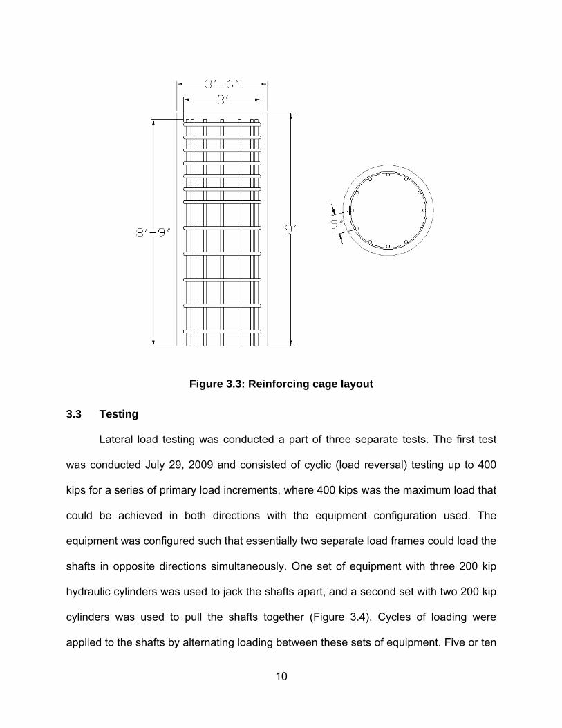
3.2 Shaft Details

The shafts were 42 inches in diameter and cast in sockets approximately six feet

deep for the north shaft and seven feet deep for the south shaft. Shaft reinforcement

consisted of twelve #11 longitudinal bars and hoops made of #5 bars on with one foot

spacing within the socket and a spacing of approximately 6 inches above ground at the

point of load application (Figure 3.3). The load was applied approximately one foot

above ground level. Concrete was KDOT standard drilled shaft mix.

Figure 3.2: Site map (Google Maps, 2010)

Approximate location of test

10  

 

3.3 Testing

Lateral load testing was conducted a part of three separate tests. The first test

was conducted July 29, 2009 and consisted of cyclic (load reversal) testing up to 400

kips for a series of primary load increments, where 400 kips was the maximum load that

could be achieved in both directions with the equipment configuration used. The

equipment was configured such that essentially two separate load frames could load the

shafts in opposite directions simultaneously. One set of equipment with three 200 kip

hydraulic cylinders was used to jack the shafts apart, and a second set with two 200 kip

cylinders was used to pull the shafts together (Figure 3.4). Cycles of loading were

applied to the shafts by alternating loading between these sets of equipment. Five or ten

Figure 3.3: Reinforcing cage layout

11  

cycles were applied at each primary load increment. Additional measurements were

taken at intermediate increments.

 

Load was measured using two separate systems, load cells and hydraulic

pressure. The hydraulic pressure was monitored by gauge and by pressure transducer.

The load cells were limited to a capacity of 400 kips and served as a backup to the

pressure transducer and gauge. Deformation was measured at two locations on each

shaft with UniMeasure P510 string pots fixed to reference beams and inclinometer

measurements in each shaft. Pressure transducer, string pot, and load cell data was

recorded automatically on a laptop computer. Photogrammetry was used as a backup

system. Pressure transducer and string pot information was recorded by a laptop and

Figure 3.4: Test 1 setup

Inclinometer casing

reference beam 

reference beam 

string pots 

string pots 

Load rods (4 on each side)

hemispherical ball

Load cells cylinders pull shafts together 

cylinders push shafts apart

12  

data acquisition system. Inclinometer data was recorded by KDOT personnel with a

data logger prior to each test and after each set of load cycles.

The second test was conducted on November 10, 2009. For this test the

equipment was reconfigured so that all five cylinders could be used together to load the

shafts to failure as shown in Figure 3.5. Repeated loads were applied at 600 and 800

kip load levels with 10 cycles at each load step. As loading continued above 800 kips,

one of the loading beams began to yield, forcing the test to be stopped.

The yielding beam was reinforced and the test was restarted on December 21,

2009. Loading proceeded to failure at approximately 1,000 kips for both shafts.

 

   Figure 3.5: Loading configuration for Tests 2 and 3

13  

CHAPTER 4 - RESULTS OF TESTING

This chapter contains a discussion of the testing of the host rock, concrete for the

shaft, and the deformations observed during the testing.

4.1 Rock and Materials Testing

Two borings were made and cores recovered at the site in the vicinity of the rock

sockets. The boring logs and are presented in Appendix A. Little soil overburden was

present on the site. Rock consisted of a 1.5 to 2 feet of sandstone over limestone,

however the soil and sandstone were removed so all testing took place in the limestone.

A number of rock samples were tested in unconfined compression and the results are

reported in Appendix A. Seven of these tests were at elevations considered relevant to

this study and the results of those tests are reported in Table 4.1.

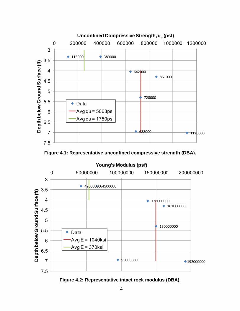
This rock core data was considered to represent two layers; an upper, more

weathered layer and a lower more competent layer. Representative values for

unconfined compressive strength (qu) and initial intact rock modulus (E) were estimated

from plots so that vertical spatial variation could be considered. These plots are shown

in Figures 4.1 and 4.2, and were developed by Dan Brown and Associates (DBA).

 Sample No. 

Depth (Ft) Unconfined Compression 

qu (psi) 

Elastic Modulus  E (ksi) 

Dry Density γd 

(pcf) 

Moisture Percent w% 

Upper 

Layer  14‐1‐2  3.33  799  292  154.4  2.7 

15‐1‐3  3.33  2701  448  149.5  4.3 

Lower Layer  14‐2‐1  4.05  4458 958 150.6  3.7

14‐2‐2  7.03  7778 1333 157.5  2.1

15‐2‐1  4.30  5979 1118 156.9  2.7

15‐2‐2  5.30  5056 1042 156.0  3.1

15‐2‐3  6.95  4778 660 152.2  4.6

Table 4.1: Rock Core Test Data used for Analysis

14  

 

 

115000

642000

1120000

389000

861000

728000

688000

3

3.5

4

4.5

5

5.5

6

6.5

7

7.5

0 200000 400000 600000 800000 1000000 1200000D

ep

th b

elo

w G

rou

nd

Su

rfa

ce

(ft)

Unconfined Compressive Strength, qu (psf)

Data

Avg qu = 5068psi

Avg qu = 1750psi

42000000

138000000

192000000

64500000

161000000

150000000

95000000

3

3.5

4

4.5

5

5.5

6

6.5

7

7.5

0 50000000 100000000 150000000 200000000

De

pth

be

low

Gro

un

d S

urf

ac

e (f

t)

Young's Modulus (psf)

Data

Avg E = 1040ksi

Avg E = 370ksi

Figure 4.1: Representative unconfined compressive strength (DBA).

Figure 4.2: Representative intact rock modulus (DBA).

15  

Concrete cylinders were taken when the shafts were constructed and the 28-day

curing strength was determined. Values of 7,588 psi and 7,020 psi were measured for

an average of 28-day strength of 7,304 psi. Given the additional strength gain that

should have occurred prior to actual testing of the shafts and based on cylinders from a

concurrent study, a model strength of 7,500 psi was used.

4.2 Field Data

Three separate test events were conducted on the shafts as described in

Chapter 3. Figures 4.3 and 4.4 show the deformation for each test event as measured

by the top string pots. Data for individual cycles are not shown in these graphs. These

figures both show increasing rates of deflection with load to failure, which occurred at

approximately 1,000 kips for both shafts. Data for the lower string pots on each shaft

were similar.

These figures, after adjustments for the vertical position of the string pots, served

as the primary physical test information used to calibrate the LPILE models. The string

pot deformation data was checked against inclinometer data, and inclinometer data was

used as an absolute reference when combining information from Test 1, 2, and 3.

Additional observations can be made in addition to the general trend of the data.

Little to no permanent accumulation of deformation was observed for cyclic loading of

the shafts at 400 kips or lower. Accumulation of deformation was significantly greater at

the 800 kip loading increment than for the 600 kip loading increment. The south shaft

deformed significantly more than the north shaft under the same loading, reaching a

deformation of nearly 0.7 inches after cycling at 800 kips while the north shaft had a

deformation of approximately 0.3 inches at the same point. This may have been due to

16  

natural material variability, or to a road cut that was present approximately 20 feet

behind the south shaft in the direction of loading, which could have made it possible for

sliding along a weak plane to have occurred in that direction.

 

0

200

400

600

800

1000

1200

0 0.1 0.2 0.3 0.4 0.5 0.6

Load

(ki

ps)

Deflection (inches)

Test 1

Test 2

Test 3

Accumulated deformation during repeated loading

Figure 4.3: Deflection of the north shaft as measured by the top string pot

17  

 

For the north shaft there was no permanent deformation between Test 1 and 2,

and there may have even been a small additional rebound between testing events.

However, during Test 2 the shaft behaved as if it had a lower modulus in the early

stages than it had during Test 1, but then stiffened when loading exceeded 600 kips.

For the south shaft this behavior was reversed. The shaft experienced a small

permanent deformation as a result of Test 1 and had higher modulus during reloading

up to 600 kips. The behavior of the south shaft is consistent with the loading of many

geomaterials, where it would be expected that some permanent deformation would be

made to the material during the initial loading, and during repeated loadings the

geomaterial would have elastic behavior with a higher modulus in that loading range.

The mechanics behind the behavior of the north shaft are not well understood, but may

0

200

400

600

800

1000

1200

-1.2 -1.1 -1 -0.9 -0.8 -0.7 -0.6 -0.5 -0.4 -0.3 -0.2 -0.1 0

Load

(ki

ps)

Deflection (inches)

Test 1

Test 2

Test 3

Accumulated deformation during repeated loading

Figure 4.4: Deflection of the south shaft with load as measured by the top string pot

18  

be behavior similar to a wobbly tooth where the shaft gradually rebounded to its original

position under small lateral earth pressures; but was quickly moved past its maximum

deformation level from Test 1 (550 kips) under loading of only 300 kips in Test 2.

4.3 Behavior During Cycling

Cyclic loading (load reversal) was applied at loads of 200, and 400 kips for five

cycles each during Test 1. Ten cycles were applied for a load of 300 kips. During Test 2

the load frame was reconfigured for repeated loading where loads were applied and

released in the same direction for ten cycles at loads of 600 and 800 kips. This data is

presented for the string pots on the south shaft in Figures 4.5 and 4.6, except for two

cycles at 200 kips which were not recorded.

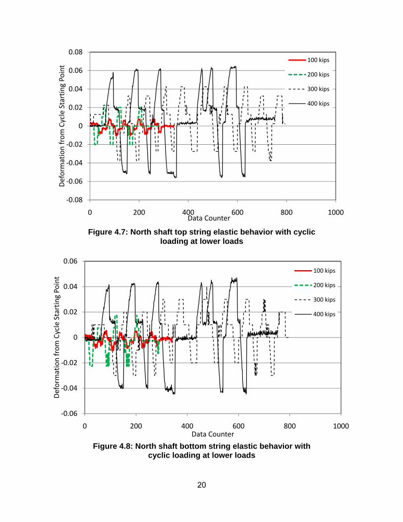
Figures 4.7 and 4.8 show more detail for the deformations for the cyclic loading

of the north shafts. For these shafts the deformation was reset to zero at the beginning

of each set of cycles. These figures show that elastic behavior was observed for cycling

below 400 kips.

19  

 

 

0

100

200

300

400

500

600

700

800

900

-0.8 -0.7 -0.6 -0.5 -0.4 -0.3 -0.2 -0.1 0

Load

(ki

ps)

Deflection (inches)

cycle 1cycle 2cycle 3cycle 4cycle 5cycle 6cycle 7cycle 8cycle 9cycle 10

accumulateddeformation 

during repeated loading elastic

behavior during cycling

0

100

200

300

400

500

600

700

800

900

-0.8 -0.7 -0.6 -0.5 -0.4 -0.3 -0.2 -0.1 0

Load

(ki

ps)

Deflection (inches)

cycle 1cycle 2cycle 3cycle 4cycle 5cycle 6cycle 7cycle 8cycle 9cycle 10

accumulateddeformation 

during repeated loading

elasticbehavior during cycling

Figure 4.5: South shaft top string accumulated deformation with cyclic and repeated loading

Figure 4.6: South shaft bottom string accumulated deformation with cyclic and repeated loading

20  

 

 

‐0.08

‐0.06

‐0.04

‐0.02

0

0.02

0.04

0.06

0.08

0 200 400 600 800 1000

Deform

ation from Cycle Starting Po

int

Data Counter

100 kips

200 kips

300 kips

400 kips

‐0.06

‐0.04

‐0.02

0

0.02

0.04

0.06

0 200 400 600 800 1000

Deform

ation from Cycle Starting Po

int

Data Counter

100 kips

200 kips

300 kips

400 kips

Figure 4.7: North shaft top string elastic behavior with cyclic loading at lower loads

Figure 4.8: North shaft bottom string elastic behavior with cyclic loading at lower loads

21  

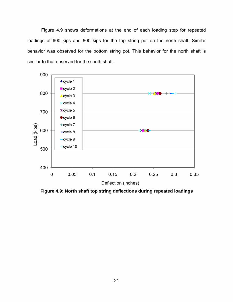
Figure 4.9 shows deformations at the end of each loading step for repeated

loadings of 600 kips and 800 kips for the top string pot on the north shaft. Similar

behavior was observed for the bottom string pot. This behavior for the north shaft is

similar to that observed for the south shaft.

 

 

 

 

   

400

500

600

700

800

900

0 0.05 0.1 0.15 0.2 0.25 0.3 0.35

Load

(ki

ps)

Deflection (inches)

cycle 1

cycle 2

cycle 3

cycle 4

cycle 5

cycle 6

cycle 7

cycle 8

cycle 9

cycle 10

Figure 4.9: North shaft top string deflections during repeated loadings

22  

CHAPTER 5 - LPILE MODELING

5.1 Modeling Parameters

The rock-socket test data was modeled using the commercial program LPILE for

the purpose of identifying appropriate p-y modeling parameters for limestone in Kansas.

The “weak rock” model contained within LPILE combined with a Type 3 analysis, which

considers non-linear bending, was determined to be the most appropriate model based

on recommendations from Dan Brown and Associates (Paul Axtell, personal

communication). Properties used in the modeling are presented in Table 5.1.

Shaft Properties

Shaft Diameter 42 inches Concrete Strengths 7500 psi Longitudinal Reinforcement 12 - #11 bars Distance from pile top (point of loading) to ground surface

12 inches

Yield stress of steel 60,000 psi Steel modulus 29,000,000 psi Rock Properties

Upper Layer Lower Layer Intact Rock Strength 1750 psi 5068 psi Intact Rock Modulus 370 ksi 1040 ksi k 0.0005 0.0005

 

Table 5.1: LPILE Modeling Parameters

23  

 

 

The layout of the model is shown in Figure 5.1. For modeling purposes the top of

the shaft is the point of load application.

Once the geometry and reinforcement of the shaft are determined, there are only

two remaining parameters that must be selected by the modeler. The value of k is

adjustable, and the value of 0.0005 that was used is within the recommended range

(Reese et al 2004). There is also some justification for reducing the rock modulus

because the modulus of the rock mass should be less than the modulus of intact

samples, however this should be accounted for to some degree by the inclusion of RQD

within the model.

Figure 5.1: General layout of shaft in model

24  

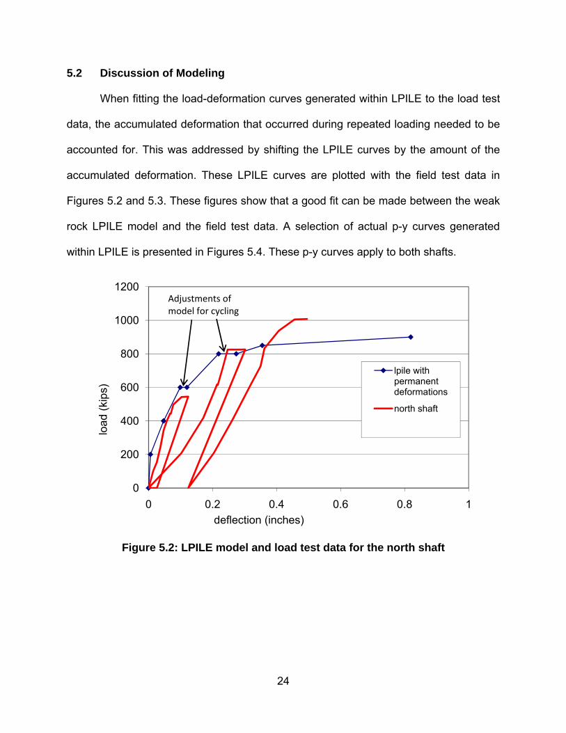
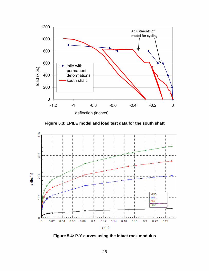
5.2 Discussion of Modeling

When fitting the load-deformation curves generated within LPILE to the load test

data, the accumulated deformation that occurred during repeated loading needed to be

accounted for. This was addressed by shifting the LPILE curves by the amount of the

accumulated deformation. These LPILE curves are plotted with the field test data in

Figures 5.2 and 5.3. These figures show that a good fit can be made between the weak

rock LPILE model and the field test data. A selection of actual p-y curves generated

within LPILE is presented in Figures 5.4. These p-y curves apply to both shafts.

 

0

200

400

600

800

1000

1200

0 0.2 0.4 0.6 0.8 1

load

(ki

ps)

deflection (inches)

lpile with permanent deformations

north shaft

Adjustments of model for cycling

Figure 5.2: LPILE model and load test data for the north shaft

25  

 

 

0

200

400

600

800

1000

1200

-1.2 -1 -0.8 -0.6 -0.4 -0.2 0

load

(ki

ps)

deflection (inches)

lpile with permanent deformationssouth shaft

Adjustments of model for cycling

Figure 5.3: LPILE model and load test data for the south shaft

Figure 5.4: P-Y curves using the intact rock modulus

26  

While the pile head deformations and ultimate load are approximated well by the

models shown in Figures 5.2 and 5.3, deformation of the shaft does not match

particularly well with the inclinometer data. Figure 5.5 shows the predicted deformation

of the north shaft from the LPILE model. This figure shows essentially no bending of the

shaft below a depth of 2.5 feet (3.5 feet below the point of load application). This is not

consistent with the inclinometer data taken during the test (Figure 5.6), which shows

movement of the shaft throughout the length of the shaft. Note, when considering the

inclinometer data it is important to remember that the base of the shaft is assumed to

have zero horizontal movement. This does not have to be the case as the shaft bottom

will sometimes rotate back in the direction of loading. The lack of bending in the model

suggests that the modulus used for the rock in the model is higher than the actual rock

modulus. This is reasonable given that the modulus of a rock mass would be expected

to be lower than the modulus of intact rock samples, and while the Reese method

accounts for this to some degree, it may not be sufficient. Additionally, the modulus of

the rock mass may have degraded further during repeated loading.

 

27  

 

Figure 5.5: Predicted deformation of the north shaft in LPILE with intact rock modulus

28  

 

Figure 5.6: Inclinometer data for the north shaft during and after Test 3

29  

Therefore the analysis was redone using a modulus that was 1/100 of the intact

rock modulus for the north shaft and 1/150 of the intact rock modulus for the south

shaft. The predicted load-deformation curves are shown in Figures 5.7 and 5.8. No

adjustment is made in these figures for accumulated deformations due to cycling as this

is assumed to be accounted for in the reduced modulus. These figures show the model

predicts the general load-deflection trend well, although it underpredicts the ultimate

capacity of the shafts by about 10 percent. Figure 5.9 shows the predicted bending of

the shaft. This figure shows that predicted lateral movement at the top of the shaft is

nearly identical to the field data and that some bending occurs all the way to the bottom

of the shaft, and therefore represents a better match with the observed data.

 

0

200

400

600

800

1000

1200

0 0.1 0.2 0.3 0.4 0.5 0.6 0.7

load

(ki

ps)

deflection (inches)

lpile with modified modulus

Figure 5.7: LPILE model of north shaft with a reduced rock modulus with field data

30  

 

 

0

200

400

600

800

1000

1200

-1.2 -1 -0.8 -0.6 -0.4 -0.2 0

load

(ki

ps)

deflection (inches)

lpile with modified modulus

Figure 5.8: LPILE model of south shaft with a reduced rock modulus with field data

Figure 5.9: Predicted deformation of the north shaft in LPILE using 1/100 of the intact rock modulus

31  

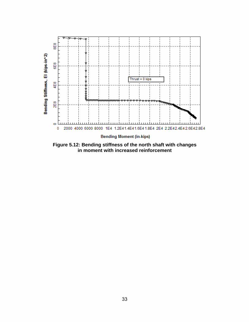
5.3 Effects of Changing Shaft Reinforcement

Figure 5.5 shows sharp bending in the middle of the north shaft as failure is

approached at 900 kips in the model, and Figure 5.10 shows shaft stiffness approaching

zero as the bending moment approached 20,000 in-kips, indicating that failure of the

shaft materials was a major factor in shaft capacity. Therefore another model was

created to explore the potential benefits of changing the reinforcement.

For this model the reinforcement was changed to #14 bars from #11. This

change resulted in an increase in predicted capacity to 1,150 kips from 900 kips.

Deflections were predicted to be less than 0.1 inch for a load of 900 kips (Case 5,

Figure 5.11), and 0.37 inches at 1,150 kips. The increase in steel enabled the shaft to

tolerate bending moments approaching 28,000 in-kips before stiffness went to zero.

Similarly, if the steel reinforcement is stronger than the design value of 60,000

psi, the model capacity of the shaft will increase. If a value of 70,000 ksi is used for the

steel, the ultimate capacity increases to approximately 1,000 kips, which is the value

observed in the field.

32  

 

 

Figure 5.10: Bending stiffness of the north shaft with changes in moment

Figure 5.11: Predicted deflection for the north shaft with increased reinforcement

33  

 

   

Figure 5.12: Bending stiffness of the north shaft with changes in moment with increased reinforcement

34  

CHAPTER 6 - CONCLUSIONS AND RECOMMENDATIONS

Two 42-inch diameter drilled shafts in limestone were laterally loaded to failure.

Cyclic and repeated loading steps were conducted at a series of load steps prior to

failure. The following conclusions were drawn from the field data.

The ultimate capacity of both shafts was approximately 1,000 kips.

The ultimate capacity was reached at approximately 0.45 inches for the

north shaft and 0.95 inches for the south shaft. Both of these deformation

values include deformation that accumulated during periods of repeated

loading. Maximum deformations for static load test conditions would likely

have been less.

Deformations for the south shaft may have been affected (increased) by

the presence of a road cut approximately 20 feet behind the shaft.

The shafts behaved in an elastic manner for five cycles of loading at 200

and 400 kips (40% of ultimate load) and 10 cycles at 300 kips.

The shafts experienced permanent, accumulating deformations for

repeated loading at 600 kips (60% of ultimate load), and even greater

deformations at 800 kips.

The resulting field data was modeled using the commercial software LPILE. The

model used was a Type 3 analysis of shafts in the weak rock model described in

Chapter 2. The following conclusions were developed based on the modeling.

The ultimate capacity and ground line deformations could be modeled

reasonably well using the weak rock model contained within LPILE.

Predicted ultimate capacity was within 10 percent of field measurements

35  

and the slope of the load-deformation curve (modulus) was consistent with

field data when accumulated deformations were accounted for.

For this model, most of the data to be entered is driven by the material

properties and geometry, which makes construction of the model very

straightforward.

The user does have control over the value of krm. The authors used the

value of 0.0005 for this parameter, which is the upper end of the

recommended range.

The model prediction of shaft bending showed minimal bending in the

lower half of the shaft. Reducing the value of the rock modulus resulted in

an increase in the predicted bending of the shaft, which better matched

inclinometer measurements and did not change the ultimate capacity of

the shaft significantly. A reduction of the modulus may be warranted given

the rock mass likely accumulated damage during the repeated loading

steps, which would have lowered the modulus of the rock mass.

Increasing the strength of the reinforcing steel in the model reduced the

predicted deformation and increased ultimate shaft capacity.

Based on these conclusions, the following preliminary recommendations are

made for modeling of limestone in Kansas. They are considered preliminary because

they are based on a single test program and should be updated as more data becomes

available.

Use of the weak rock model included within LPILE is recommended for

Kansas limestone.

36  

Within this model it is recommended that a value of 0.0005 be used for krm

if no other information is available.

It is also recommended that for cyclic or repeated loading design where

the number of cycles is expected to be relatively small (i.e. extreme

events), the limestone can be considered elastic for loads of less than

40% of the ultimate load.

If the intact rock modulus is the basis for selecting the rock modulus value

used in LPILE, use of a reduced value may be warranted to more

accurately model shaft bending.

   

37  

REFERENCES

Google Maps (2010). http://maps.google.com/maps. Google, Inc.

Reese, L.C. (1997). Analysis of Laterally Loaded Piles in Weak Rock. Journal of Geotechnical and Geoenvironmental Engineering. ASCE. Reston, Virginia. v123 n11. 1010-1017.

Reese, L.C., S.T. Wang, W.M. Isenhower, and J.A. Arrellaga (2004). Technical Manual, LPILE Plus 5.0 for Windows, A Program for the Analysis of Piles and Shafts Under Lateral Loads. Ensoft, Inc. Austin TX.

38  

APPENDIX A*

*Appendix A is available on CD only upon request.

Please send your request to library@ksdot.org.