Lateral Capacity of Short Rock Sockets in Weak Rock: A ...docs.trb.org/prp/11-2791.pdf · 2 1 2 3 INTRODUCTION 4 This paper contains the results from a full-scale lateral load test

Lateral Resistance of Short Rock Sockets in Weak Rock: a Case History

Text word count: 4140

Number of figures and tables: 13 Robert L. Parsons PhD, P.E (Corresponding Author) Associate Professor Department of Civil, Environmental and Architectural Engineering 1530 W 15th St., Room 2150 University of Kansas Lawrence, KS 66045 [email protected] (785) 864-2946 Matthew C. Pierson Assistant Professor, Cooperative Engineering Program Kemper Hall, Room 226 Missouri State University 901 S. National Ave. Springfield, MO 65897 [email protected] 785-393-2427 Isaac Willems Graduate Student Department of Civil, Environmental and Architectural Engineering 1530 W 15th St., Room 2150 University of Kansas Lawrence, KS 66045 [email protected] (309) 258-7743 Jie Han PhD, P.E Associate Professor Department of Civil, Environmental and Architectural Engineering 1530 W 15th St., Room 2150 University of Kansas Lawrence, KS 66045 [email protected] (785) 393-3714 James J. Brennan Assistant Geotechnical Engineer Kansas Department of Transportation 2300 Van Buren Topeka, KS 66611-1195 [email protected] (785) 296-3008

TRB 2011 Annual Meeting Paper revised from original submittal.

1

1

2

Lateral Capacity of Short Rock Sockets in Weak Rock: a Case History 3

4

5

ABSTRACT 6

The results from full-scale cyclic and repeated lateral load testing of two short rock sockets in 7

weak rock and the recommendations developed for p-y analysis using those results are presented. 8

Two drilled shafts were constructed in rock sockets 42 inches in diameter to depths of 9

approximately seven feet in limestone in Wyandotte County, Kansas. The shafts were loaded 10

laterally during three separate test events. The shafts were tested under cyclic loading (load 11

reversal) for loads up to 400 kips, repeated loading in one direction up to 820 kips, and to failure 12

near 1,000 kips. 13

Test data showed that socket behavior was essentially elastic during cyclic loading for 14

loads of 400 kips (40% of nominal resistance) and lower. The shafts experienced permanent, 15

accumulating deformations during repeated loading to 610 and 820 kips. 16

Modeling of the results showed the lateral load behavior could be effectively modeled in 17

LPILE using the Reese “weak rock” model included with LPILE software. Recommendations 18

for use in modeling are presented. 19

20


2

1

2

INTRODUCTION 3

This paper contains the results from a full-scale lateral load test of two drilled shafts constructed 4

in short rock sockets in weak limestone, and the development of recommendations for p-y 5

analysis using those results. Lateral nominal resistance of drilled shafts is of particular interest 6

with regard to bridge foundations because of the significant loading conditions they experience, 7

particularly during scour events. Lateral nominal resistance may be estimated during the design 8

process by several methods, with one of the most common being a p-y analysis. P-y curves vary 9

among soil types and rock formations, although general curves have been developed and are 10

available for use in widely available software packages such as COM624 (public domain) and 11

LPILE (proprietary software, Ensoft). 12

The purpose of this research was to test the lateral capacity and develop p-y curves for 13

short rock sockets in weak rock. Two shafts 42 inches in diameter were constructed to depths of 14

six and seven feet in limestone in Wyandotte County, Kansas. All overburden material was 15

removed prior to construction. The shafts were loaded laterally during three separate test events. 16

During the first event, the shafts were loaded in a cyclic manner (load reversal) at multiple 17

increments up to 400 kips. The cyclic loading was of interest because of the potential for lateral 18

loading in alternating directions on shafts supporting integral abutments. The shafts were then 19

loaded in one direction to 550 kips. The equipment was then reconfigured and the shafts were 20

loaded to 820 kips with repeated loading-unloading cycles at 610 and 820 kips. The loading 21

frame was then reinforced and the shafts were loaded to failure, which occurred near 1,000 kips. 22

A description of the testing, analysis, and p-y curve recommendations is presented in Parsons et 23

al. (1). 24

Analysis of the data showed that commonly used p-y curves included within the LPILE 25

software could be used to develop an accurate model of the static behavior of the shafts. Cyclic 26

loading of the shafts had little effect on shaft resistance at lower loads; however permanent 27

deformation began to accumulate at loading levels between 40 and 60 percent of nominal 28

resistance. 29

THEORETICAL BACKGROUND 30

This section contains an abridged discussion of the p-y curve method. For a more detailed 31

discussion of the p-y curve method the reader is referred to Reese et al. (2). 32

For the p-y method the pile-soil interaction is modeled as a series of nonlinear springs, 33

where “p” represents lateral load per unit length on a spring and “y” represents displacement of 34


3

the spring. The non-linear relationship is captured by the secant modulus Er, which decreases 1

according to some function, such as a hyperbolic function, as displacement increases. 2

The p-y method was extended to the analysis of single rock-socketed drilled shafts under 3

lateral loading by Reese (3). Reese’s criteria, which he considered “interim” criteria pending the 4

availability of more test data, include consideration of the secondary structures of rock masses 5

using a rock strength reduction factor determined from the Rock Quality Designation (RQD). 6

Other criteria used for generating p-y curves have subsequently been developed (4, 5). Reese’s 7

criteria have been incorporated into LPILE v 5.0 Plus (2), and were used for the analysis 8

described in this paper. 9

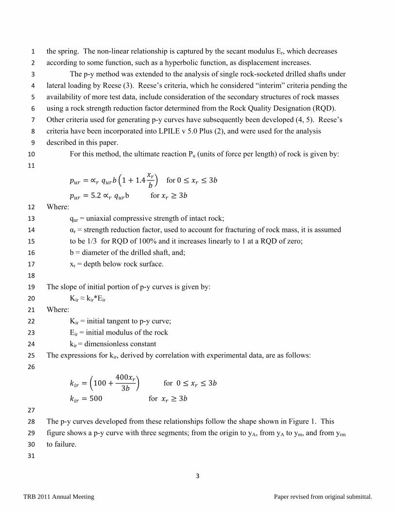
For this method, the ultimate reaction Pu (units of force per length) of rock is given by: 10

11

1 1.4 for 0 3

5.2 b for 3

Where: 12

qur = uniaxial compressive strength of intact rock; 13

αr = strength reduction factor, used to account for fracturing of rock mass, it is assumed 14

to be 1/3 for RQD of 100% and it increases linearly to 1 at a RQD of zero; 15

b = diameter of the drilled shaft, and; 16

xr = depth below rock surface. 17

18

The slope of initial portion of p-y curves is given by: 19

Kir ≈ kir*Eir 20

Where: 21

Kir = initial tangent to p-y curve; 22

Eir = initial modulus of the rock 23

kir = dimensionless constant 24

The expressions for kir, derived by correlation with experimental data, are as follows: 25

26

100400

3 for 0 3

500 for 3

27

The p-y curves developed from these relationships follow the shape shown in Figure 1. This 28

figure shows a p-y curve with three segments; from the origin to yA, from yA to ym, and from yrm 29

to failure. 30

31


4

1

2

3

4

5

6

7

8

9

10

11

12

13

14

Figure 1. Sketch of p-y curve for weak rock (adapted from Reese [3]) 15

16

The equations relating p and y for the curve in Figure 1 are as follows: 17

18

for y ≤ yA

2

.

for y > yA, p <pur

for y > 16yrm

19

and 20

= 21

22

where 23

24

krm = a constant between 0.0005 and 0.00005 that controls the overall stiffness of the p-y curves, 25

and; 26

27

2 .

.

28

29

30

Kirpur

yrm yA y


5

FIELD TESTING 1

2

Site Investigation 3

The shafts were constructed in the fall of 2007 in the northeast quadrant of the intersection of I-4

70 and I-435 in Wyandotte County, Kansas. The sockets were in the Plattsburg Limestone. Two 5

borings were made and cores were recovered at the site in the vicinity of the rock sockets. The 6

site geology consisted of minimal to no soil overburden, 1.5-2.5 feet of weathered to 7

unweathered sandstone over weak limestone. The overburden and sandstone were removed so 8

the sockets were entirely in limestone. More detailed information is available in Parsons et al. 9

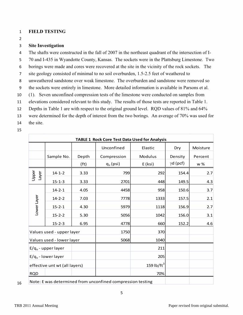
(1). Seven unconfined compression tests of the limestone were conducted on samples from 10

elevations considered relevant to this study. The results of those tests are reported in Table 1. 11

Depths in Table 1 are with respect to the original ground level. RQD values of 81% and 64% 12

were determined for the depth of interest from the two borings. An average of 70% was used for 13

the site. 14

15

Unconfined Elastic Dry Moisture

Sample No. Depth Compression Modulus Density Percent

(ft) qu (psi) E (ksi) d (pcf) w %

14‐1‐2 3.33 799 292 154.4 2.7

15‐1‐3 3.33 2701 448 149.5 4.3

14‐2‐1 4.05 4458 958 150.6 3.7

14‐2‐2 7.03 7778 1333 157.5 2.1

15‐2‐1 4.30 5979 1118 156.9 2.7

15‐2‐2 5.30 5056 1042 156.0 3.1

15‐2‐3 6.95 4778 660 152.2 4.6

Values used ‐ upper layer 1750 370

Values used ‐ lower layer 5068 1040

E/qu ‐ upper layer 211

E/qu ‐ lower layer 205

effective unt wt (all layers) 159 lb/ft3

RQD 70%

Note: E was determined from unconfined compression testing

Lower Layer

Upper

Layer

TABLE 1 Rock Core Test Data Used for Analysis

16


6

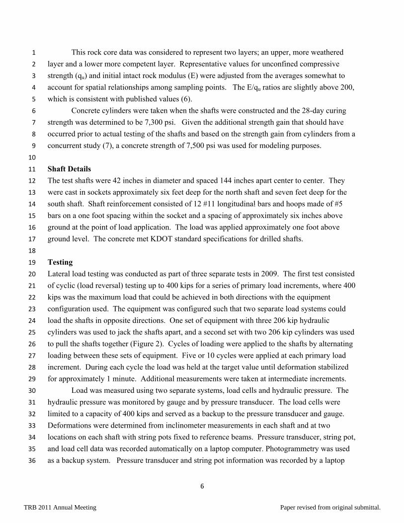
This rock core data was considered to represent two layers; an upper, more weathered 1

layer and a lower more competent layer. Representative values for unconfined compressive 2

strength (qu) and initial intact rock modulus (E) were adjusted from the averages somewhat to 3

account for spatial relationships among sampling points. The E/qu ratios are slightly above 200, 4

which is consistent with published values (6). 5

Concrete cylinders were taken when the shafts were constructed and the 28-day curing 6

strength was determined to be 7,300 psi. Given the additional strength gain that should have 7

occurred prior to actual testing of the shafts and based on the strength gain from cylinders from a 8

concurrent study (7), a concrete strength of 7,500 psi was used for modeling purposes. 9

10

Shaft Details 11

The test shafts were 42 inches in diameter and spaced 144 inches apart center to center. They 12

were cast in sockets approximately six feet deep for the north shaft and seven feet deep for the 13

south shaft. Shaft reinforcement consisted of 12 #11 longitudinal bars and hoops made of #5 14

bars on a one foot spacing within the socket and a spacing of approximately six inches above 15

ground at the point of load application. The load was applied approximately one foot above 16

ground level. The concrete met KDOT standard specifications for drilled shafts. 17

18

Testing 19

Lateral load testing was conducted as part of three separate tests in 2009. The first test consisted 20

of cyclic (load reversal) testing up to 400 kips for a series of primary load increments, where 400 21

kips was the maximum load that could be achieved in both directions with the equipment 22

configuration used. The equipment was configured such that two separate load systems could 23

load the shafts in opposite directions. One set of equipment with three 206 kip hydraulic 24

cylinders was used to jack the shafts apart, and a second set with two 206 kip cylinders was used 25

to pull the shafts together (Figure 2). Cycles of loading were applied to the shafts by alternating 26

loading between these sets of equipment. Five or 10 cycles were applied at each primary load 27

increment. During each cycle the load was held at the target value until deformation stabilized 28

for approximately 1 minute. Additional measurements were taken at intermediate increments. 29

Load was measured using two separate systems, load cells and hydraulic pressure. The 30

hydraulic pressure was monitored by gauge and by pressure transducer. The load cells were 31

limited to a capacity of 400 kips and served as a backup to the pressure transducer and gauge. 32

Deformations were determined from inclinometer measurements in each shaft and at two 33

locations on each shaft with string pots fixed to reference beams. Pressure transducer, string pot, 34

and load cell data was recorded automatically on a laptop computer. Photogrammetry was used 35

as a backup system. Pressure transducer and string pot information was recorded by a laptop 36


7

and data acquisition system. Inclinometer data was recorded by KDOT personnel with a data 1

logger prior to each test and after each set of load cycles. 2

3

Figure 2. Test 1 setup 4

5

For the second test the equipment was reconfigured so that all five cylinders could be 6

used together to load the shafts as shown in Figure 3. Repeated loads, which consisted of 7

loading to the target value and then reducing the load to zero, were applied at 610 and 820 kip 8

load levels with 10 cycles at each load step. As loading continued for Test 2 above 820 kips, one 9

of the loading beams began to yield, forcing the test to be stopped. 10

The yielding beam was reinforced and the test was restarted as Test 3. Loading 11

proceeded to failure at approximately 1,000 kips for both shafts. 12

13

Field Data 14

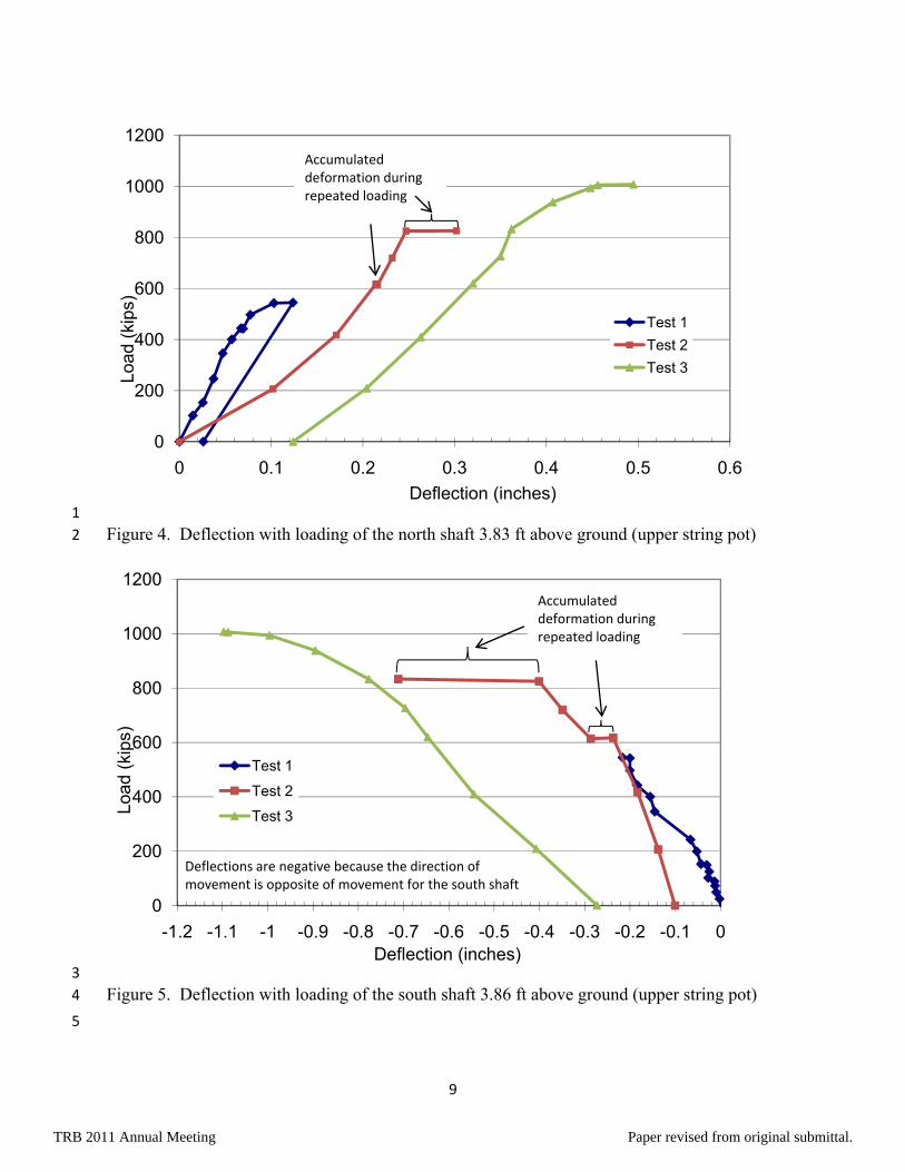
Figures 4 and 5 show the deformations that occurred during each test event as measured 15

by the top string pots, which were approximately 3.8 ft above ground level. Data for individual 16

cycles are not shown in these graphs. These figures show increasing rates of deflection with 17

increasing load to failure, which occurred at approximately 1,000 kips for both shafts. Data for 18

the lower string pots on each shaft were similar. 19

20

Inclinometer casing

reference beam

reference beam

string pots

string pots

load rods (4 on each side)

hemispherical ball

load cellscylinders push shafts together

cylinders push shafts apart


8

1

Figure 3. Loading configuration for Tests 2 and 3 2

3

These figures served as the primary physical test information used to calibrate the LPILE 4

models. The string pot deformation data was checked against inclinometer data, which was used 5

as an absolute reference when combining information from Tests 1, 2, and 3. The data plotted 6

for Tests 2 and 3 were offset based on the difference in inclinometer readings taken at the end of 7

the previous test and the beginning of the test for which the data was plotted. 8

Additional observations can be made in addition to the general trend of the data. Little 9

to no permanent accumulation of deformation was observed for cyclic loading of the shafts at 10

400 kips or lower. Accumulation of deformation was significantly greater at the 820 kip loading 11

increment than for the 610 kip loading increment. The south shaft deformed significantly more 12

than the north shaft under the same loading, reaching a deformation of nearly 0.7 inches after 13

cycling at 820 kips while the north shaft had a deformation of approximately 0.3 inches at the 14

same point. This was likely due to natural material variability; however there was a road cut that 15

was present approximately 20 feet behind the south shaft in the direction of loading which could 16

have made it possible for sliding along a weak plane to have occurred in that direction. 17

18


9

1

Figure 4. Deflection with loading of the north shaft 3.83 ft above ground (upper string pot) 2

3

Figure 5. Deflection with loading of the south shaft 3.86 ft above ground (upper string pot) 4

5

0

200

400

600

800

1000

1200

0 0.1 0.2 0.3 0.4 0.5 0.6

Load

(ki

ps)

Deflection (inches)

Test 1

Test 2

Test 3

Accumulated deformation during repeated loading

0

200

400

600

800

1000

1200

-1.2 -1.1 -1 -0.9 -0.8 -0.7 -0.6 -0.5 -0.4 -0.3 -0.2 -0.1 0

Load

(ki

ps)

Deflection (inches)

Test 1

Test 2

Test 3

Accumulated deformation during repeated loading

Deflections are negative because the direction of movement is opposite of movement for the south shaft


10

For the north shaft there was no permanent deformation between Tests 1 and 2, and there 1

may have been a small rebound between testing events. However, during Test 2 the shaft 2

behaved as if it had a lower modulus in the early stages than it had during Test 1, but then 3

stiffened when loading exceeded 600 kips. For the south shaft this behavior was reversed. The 4

shaft experienced a small permanent deformation as a result of Test 1 and had a higher modulus 5

during reloading up to 610 kips. The behavior of the south shaft is consistent with the loading of 6

many geomaterials, where it would be expected that some permanent deformation would be 7

made to the material during the initial loading, and during repeated loadings the geomaterial 8

would have elastic behavior with a higher modulus in that loading range. The mechanics behind 9

the behavior of the north shaft are not well understood, but it may have gradually rebounded to 10

its original position under small lateral earth pressures; then quickly moved past its maximum 11

deformation level from Test 1 (550 kips) under loading of only 300 kips in Test 2. 12

13

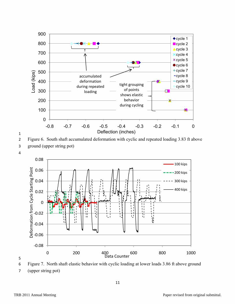
Behavior during Cycling 14

Cyclic loading (load reversal) was applied at loads of 100, 200 and 400 kips for five cycles each 15

during Test 1. Ten cycles were applied for a load of 300 kips. For Test 2 the load frame was 16

reconfigured for repeated loading where loads were applied and released in the same direction 17

for 10 cycles at loads of 610 and 820 kips. This data is presented for the top string pot on the 18

south shaft in Figure 6, except for two cycles at 200 kips which were not recorded. Similar 19

accumulating deformations for high loads were also observed for the north shaft. 20

Figure 7 shows more detail for the deformations for the cyclic loading of the north shaft. 21

For this figure the deformation was reset to zero at the beginning of each set of cycles. The 22

nearly constant amplitude for each set of cycles shows there was no significant increase in 23

movement of the shaft during cycling for loads up to 400 kips. 24

25

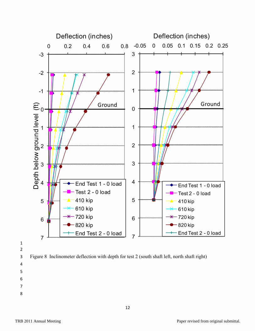
Deformations with Depth 26

Shaft deflections were monitored with depth using inclinometer measurements. The inclinometer 27

casings were installed inline with the loading direction and show that while the shafts were 28

relatively rigid for early loading, they experienced more significant bending at higher loads. The 29

inclinometer readings from Test 2 are shown in Figure 8. 30

31


11

1

Figure 6. South shaft accumulated deformation with cyclic and repeated loading 3.83 ft above 2

ground (upper string pot) 3

4

5

Figure 7. North shaft elastic behavior with cyclic loading at lower loads 3.86 ft above ground 6

(upper string pot) 7

0

100

200

300

400

500

600

700

800

900

-0.8 -0.7 -0.6 -0.5 -0.4 -0.3 -0.2 -0.1 0

Load

(ki

ps)

Deflection (inches)

cycle 1cycle 2cycle 3cycle 4cycle 5cycle 6cycle 7cycle 8cycle 9cycle 10

accumulateddeformation

during repeated loading

tight grouping of points

shows elasticbehavior

during cycling

‐0.08

‐0.06

‐0.04

‐0.02

0

0.02

0.04

0.06

0.08

0 200 400 600 800 1000

Deform

ation from Cycle Starting Po

int

Data Counter

100 kips

200 kips

300 kips

400 kips


12

-3

-2

-1

0

1

2

3

4

5

6

7

-0.05 0 0.05 0.1 0.15 0.2 0.25

Deflection (inches)

End Test 1 - 0 load

Test 2 - 0 load

410 kip

610 kip

720 kip

820 kip

End Test 2 - 0 load

Ground

1

2

Figure 8 Inclinometer deflection with depth for test 2 (south shaft left, north shaft right) 3

4

5

6

7

8

-3

-2

-1

0

1

2

3

4

5

6

7

0 0.2 0.4 0.6 0.8

De

pth

be

low

gro

un

d le

vel

(ft)

Deflection (inches)

End Test 1 - 0 load

Test 2 - 0 load

410 kip

610 kip

720 kip

820 kip

End Test 2 - 0 load

Ground


13

1

LPILE MODELING 2

3

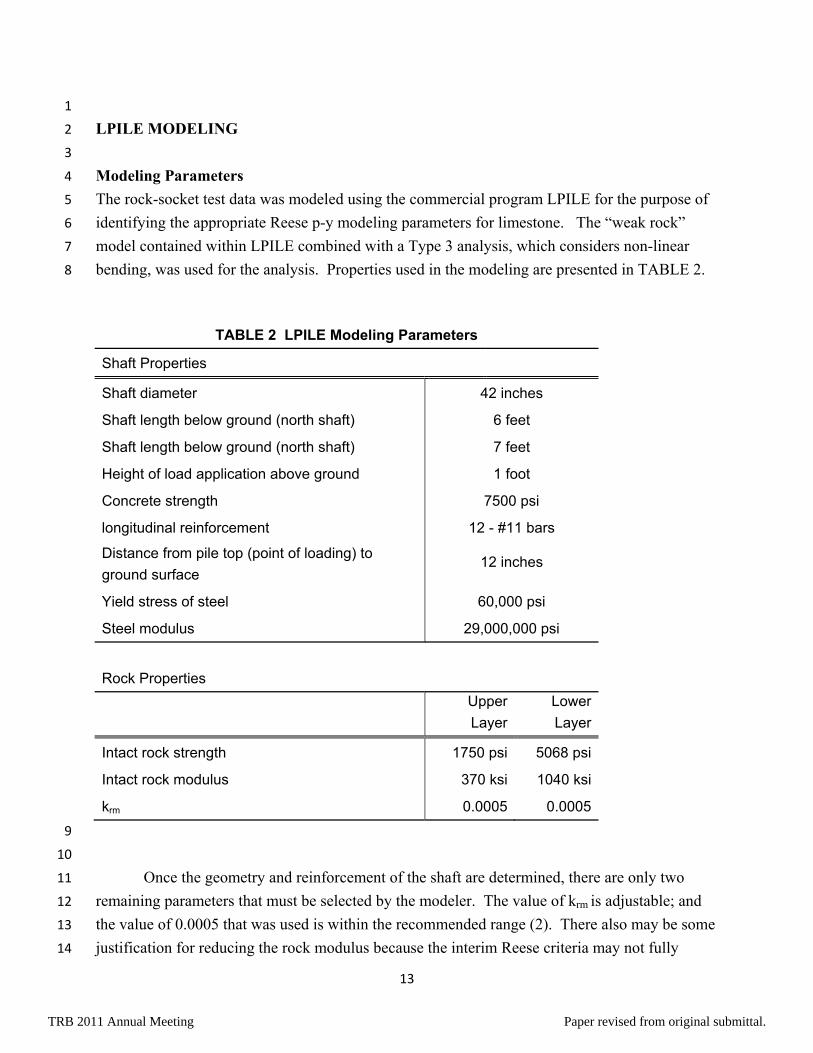
Modeling Parameters 4

The rock-socket test data was modeled using the commercial program LPILE for the purpose of 5

identifying the appropriate Reese p-y modeling parameters for limestone. The “weak rock” 6

model contained within LPILE combined with a Type 3 analysis, which considers non-linear 7

bending, was used for the analysis. Properties used in the modeling are presented in TABLE 2. 8

TABLE 2 LPILE Modeling Parameters

Shaft Properties

Shaft diameter 42 inches

Shaft length below ground (north shaft) 6 feet

Shaft length below ground (north shaft) 7 feet

Height of load application above ground 1 foot

Concrete strength 7500 psi

longitudinal reinforcement 12 - #11 bars

Distance from pile top (point of loading) to

ground surface 12 inches

Yield stress of steel 60,000 psi

Steel modulus 29,000,000 psi

Rock Properties

Upper

Layer

Lower

Layer

Intact rock strength 1750 psi 5068 psi

Intact rock modulus 370 ksi 1040 ksi

krm 0.0005 0.0005

9

10

Once the geometry and reinforcement of the shaft are determined, there are only two 11

remaining parameters that must be selected by the modeler. The value of krm is adjustable; and 12

the value of 0.0005 that was used is within the recommended range (2). There also may be some 13

justification for reducing the rock modulus because the interim Reese criteria may not fully 14


14

account for the lower modulus of the rock mass as compared with the modulus of the intact rock 1

samples as described in the next section. 2

3

Discussion of Modeling 4

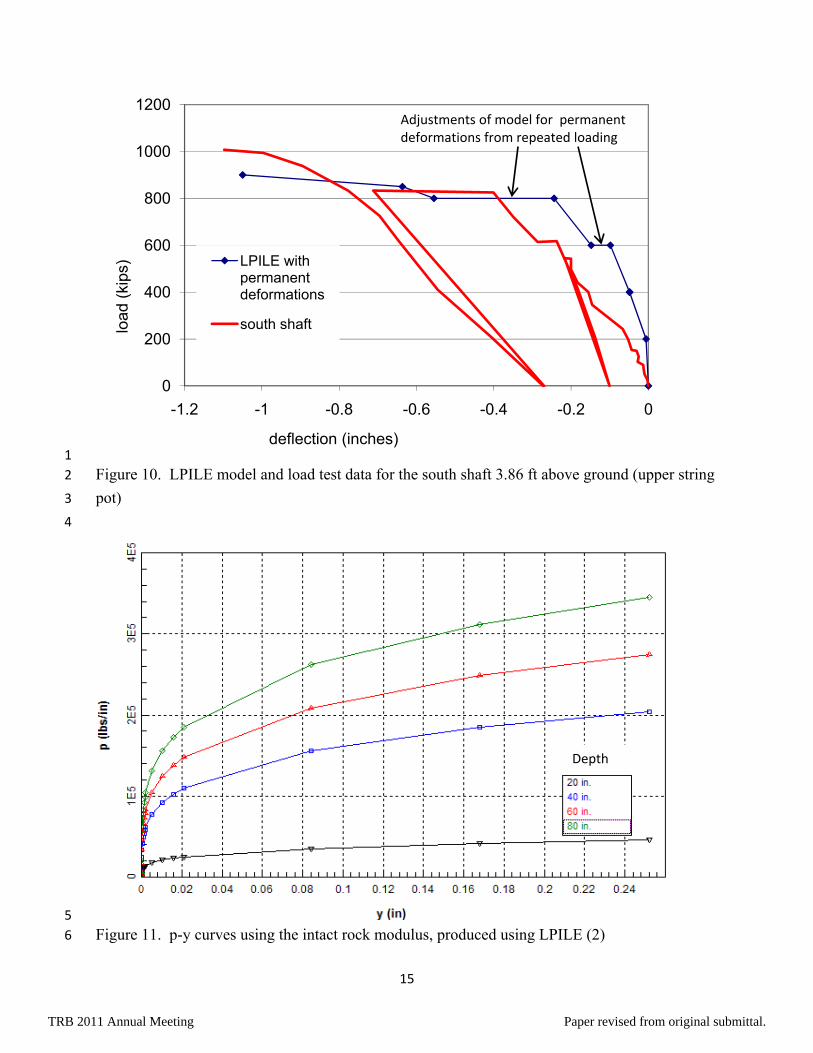
When fitting the load-deformation curves generated within LPILE to the load test data, an 5

adjustment was required to account for the accumulated deformation that occurred during 6

repeated loading. This was addressed by shifting the LPILE curves by the amount of the 7

accumulated deformation. These LPILE curves are plotted with the field test data in Figures 9 8

and 10. These figures show that a relatively good fit is obtained between the weak rock LPILE 9

model and the field test data with regard to the nominal resistance and ultimate pile head 10

deformations, with the nominal model resistance being within about 10% of the observed 11

ultimate load for both shafts. A selection of actual p-y curves generated within LPILE is 12

presented in Figure 11. These p-y curves apply to both shafts. The model results predict the 13

shafts reaching maximum moment and failing near 900 kips with nearly all bending above a 14

depth of three feet. Lengthening the shafts has minimal impact on model resistance or pile head 15

deflections. 16

17

Figure 9. LPILE model and load test data for the north shaft 3.83 ft above ground (upper string 18

pot) 19

0

200

400

600

800

1000

1200

0 0.2 0.4 0.6 0.8 1

load

(ki

ps)

deflection (inches)

LPILE with permanent deformations

north shaft

Adjustments of model for permanent deformations from repeated loading


15

1

Figure 10. LPILE model and load test data for the south shaft 3.86 ft above ground (upper string 2

pot) 3

4

5

Figure 11. p-y curves using the intact rock modulus, produced using LPILE (2) 6

0

200

400

600

800

1000

1200

-1.2 -1 -0.8 -0.6 -0.4 -0.2 0

load

(ki

ps)

deflection (inches)

LPILE with permanent deformations

south shaft

Adjustments of model for permanent deformations from repeated loading

Depth


16

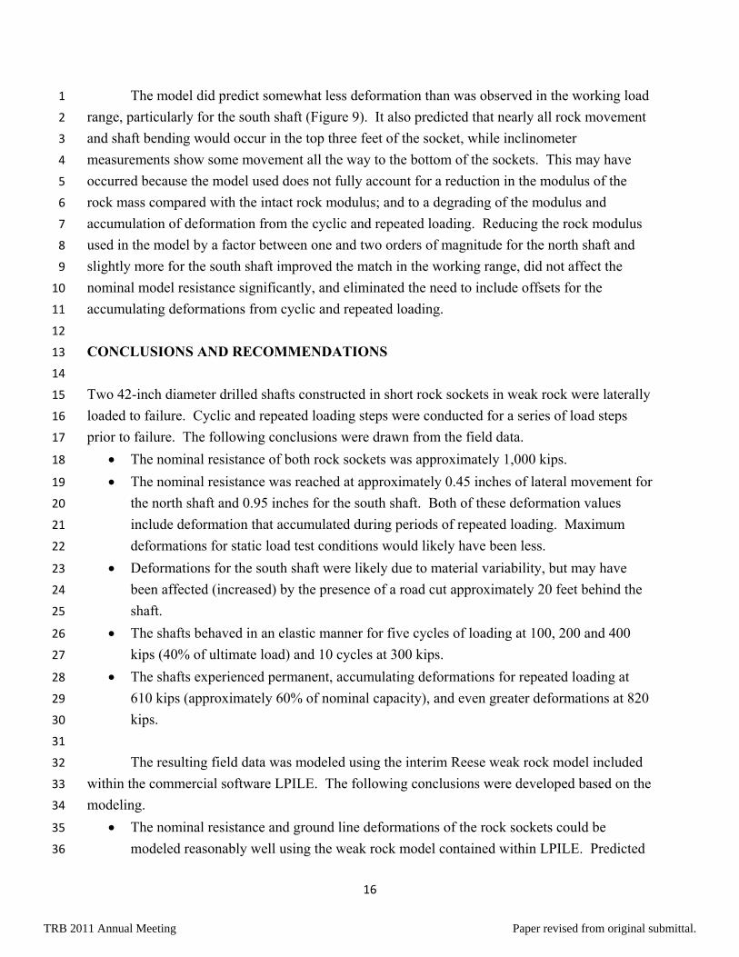
The model did predict somewhat less deformation than was observed in the working load 1

range, particularly for the south shaft (Figure 9). It also predicted that nearly all rock movement 2

and shaft bending would occur in the top three feet of the socket, while inclinometer 3

measurements show some movement all the way to the bottom of the sockets. This may have 4

occurred because the model used does not fully account for a reduction in the modulus of the 5

rock mass compared with the intact rock modulus; and to a degrading of the modulus and 6

accumulation of deformation from the cyclic and repeated loading. Reducing the rock modulus 7

used in the model by a factor between one and two orders of magnitude for the north shaft and 8

slightly more for the south shaft improved the match in the working range, did not affect the 9

nominal model resistance significantly, and eliminated the need to include offsets for the 10

accumulating deformations from cyclic and repeated loading. 11

12

CONCLUSIONS AND RECOMMENDATIONS 13

14

Two 42-inch diameter drilled shafts constructed in short rock sockets in weak rock were laterally 15

loaded to failure. Cyclic and repeated loading steps were conducted for a series of load steps 16

prior to failure. The following conclusions were drawn from the field data. 17

The nominal resistance of both rock sockets was approximately 1,000 kips. 18

The nominal resistance was reached at approximately 0.45 inches of lateral movement for 19

the north shaft and 0.95 inches for the south shaft. Both of these deformation values 20

include deformation that accumulated during periods of repeated loading. Maximum 21

deformations for static load test conditions would likely have been less. 22

Deformations for the south shaft were likely due to material variability, but may have 23

been affected (increased) by the presence of a road cut approximately 20 feet behind the 24

shaft. 25

The shafts behaved in an elastic manner for five cycles of loading at 100, 200 and 400 26

kips (40% of ultimate load) and 10 cycles at 300 kips. 27

The shafts experienced permanent, accumulating deformations for repeated loading at 28

610 kips (approximately 60% of nominal capacity), and even greater deformations at 820 29

kips. 30

31

The resulting field data was modeled using the interim Reese weak rock model included 32

within the commercial software LPILE. The following conclusions were developed based on the 33

modeling. 34

The nominal resistance and ground line deformations of the rock sockets could be 35

modeled reasonably well using the weak rock model contained within LPILE. Predicted 36


17

nominal resistance was within 10 percent of field measurements and the slope of the 1

load-deformation curve (modulus) was consistent with field data when accumulated 2

deformations were accounted for. 3

For this model, most of the data to be entered is driven by the material properties and 4

geometry, which makes construction of the model very straightforward. 5

The authors used a value of 0.0005 for krm, which is the upper end of the recommended 6

range. 7

8

Based on these conclusions, the following preliminary recommendations are made for 9

modeling of limestones. They are considered preliminary because they are based on a single test 10

program and should be updated as more data becomes available. 11

Use of the weak rock model included within LPILE for modeling short rock sockets is 12

supported by the observations from this research. 13

Within this model it is recommended that a value of 0.0005 be used for krm if no other 14

information is available. 15

It is also recommended that for cyclic or repeated loading design where the number of 16

cycles is expected to be relatively small (i.e. extreme events), the limestone can be 17

considered elastic for loads of less than 40% of the nominal resistance. 18

If the intact rock modulus is the basis for selecting the rock modulus value used in 19

LPILE, use of a reduced value may be warranted to more accurately model shaft bending 20

and deformations in the working range. 21

22

ACKNOWLEDGEMENTS 23

24

The authors wish to thank the people of the Kansas Department of Transportation for their 25

financial and logistical support that made this research possible. We particularly want to thank 26

the people of the KDOT Geotechnical Unit and KDOT Maintenance for their help in bringing 27

this project to fruition. We also wish to thank Mr. Jim Weaver of the University of Kansas (KU) 28

for his help in designing and fabricating the equipment and Mr. Justin Clay of KU for his help in 29

fabrication of the equipment for Test 1 and with some of the theoretical background presented in 30

this paper. We also wish to thank Mr. Paul Axtell and Dan Brown of Dan Brown and 31

Associates, who helped with the testing and interpretation of data. The help of all who 32

participated is greatly appreciated. 33

34

35

36


18

REFERENCES 1

2

1. Parsons, R.L., I. Willems, M.C. Pierson, and J. Han. (2010). Lateral Capacity of Rock 3

Sockets in Limestone under Cyclic and Repeated Loading. Kansas Department of 4

Transportation. 86p. 5

2. Reese, L.C., S.T. Wang, W.M. Isenhower, and J.A. Arrellaga (2004). LPILE Plus 5.0 for 6

Windows, A Program for the Analysis of Piles and Shafts Under Lateral Loads. 7

Technical Manual. Ensoft, Inc. Austin TX. 8

3. Reese, L.C. (1997). “Analysis of Laterally Loaded Piles in Weak Rock.” Journal of 9

Geotechnical and Geoenvironmental Engineering. ASCE. Reston, Virginia. v123 n11. 10

1010-1017. 11

4. Cho, K.H., S.C. Clark, B.D. Keany, M.A. Gabr, and R.H. Borden. (2001).“Laterally 12

Loaded Drilled Shafts Embedded in Soft Rock.” Soil Mechanics. Transportation 13

Research Record. Journal of the Transportation Research Board. n1772. Transportation 14

Research Board. Washington D.C. 3-11. 15

5. Gabr, M.A., R.H. Borden, K.H. Cho, S. Clark, and J.B. Nixon. (2002). P-y Curves for 16

Laterally Loaded Drilled Shafts Embedded in Weathered Rock. North Carolina 17

Department of Transportation. FHWA/NC/2002-008. 289p. 18

6. Goodman, R.E. (1989). Introduction to Rock Mechanics, 2nd ed. John Wiley and Sons. 19

New York. 562p. 20

7. Pierson, M.C., R.L. Parsons, J. Han, D. A. Brown, and W.R. Thompson. (2008). 21

Capacity of Laterally Loaded Shafts Constructed Behind the Face of a Mechanically 22

Stabilized Earth Block Wall. Kansas Department of Transportation. Report KU-07-6. 23

237p. 24

25

26


Documents

Lateral Capacity of Short Rock Sockets in Weak Rock: A ...docs.trb.org/prp/11-2791.pdf · 2 1 2 3 INTRODUCTION 4 This paper contains the results from a full-scale lateral load test