European Journal of Operational Research 204 (2010) 366–375

Contents lists available at ScienceDirect

European Journal of Operational Research

journal homepage: www.elsevier .com/locate /e jor

Interfaces with Other Disciplines

Launching new products through exclusive sales channels

Dimitrios A. Andritsos, Christopher S. Tang *

UCLA Anderson School, UCLA, 110 Westwood Plaza, Los Angeles, CA 90095, United States

a r t i c l e i n f o a b s t r a c t

Article history:Received 13 April 2009Accepted 4 November 2009

Keywords:Marketing/manufacturing interfacesRetail competitionChannel competition

0377-2217/$ - see front matter � 2009 Elsevier B.V. Adoi:10.1016/j.ejor.2009.11.002

* Corresponding author.E-mail addresses: dimitrios.andritsos.2011@anders

ctang@anderson.ucla.edu (C.S. Tang).

When launching a new product, a manufacturer usually sells it through competing retailers under non-exclusive arrangements. Recently, many new products (cellphones, electronics, toys, etc.) are soldthrough a single sales channel via an exclusive arrangement. In this paper we present two separate mod-els that examine these two arrangements. Each model is based on a Stackelberg game in which the man-ufacturer acts as the leader by setting the wholesale price and the retailers act as the followers bychoosing their retail prices. For each model, we solve the Stackelberg game by determining the manufac-turer’s optimal wholesale price and each retailer’s optimal retail price in equilibrium. Then we examinethe conditions under which the manufacturer should sell the new product through an exclusive retailer.In addition, we examine the impact of postponing the wholesale price decision and the impact of demanduncertainty on the manufacturer’s optimal profit under both arrangements.

� 2009 Elsevier B.V. All rights reserved.

1. Introduction

Launching new products is critical for manufacturers to stimu-late growth in a competitive market. Manufacturers usually devel-op new products and delegate the selling aspects to the retailerswho control the sales channels. Typically, new products are intro-duced through multiple, competing sales channels. These non-exclusive arrangements enable manufacturers to expose theirnew products to consumers through the extended reach of differ-ent channels, and provide the convenience for consumers to makepurchases through alternative channels.

Under the non-exclusive arrangements, a manufacturer sets thewholesale price and the competing retailers set their retail prices.As a result of retail price competition, consumers usually enjoy alower retail price. Hence, the non-exclusive arrangements are pre-ferred by the manufacturer and the consumers. However, theretailers are faced with the following dilemma: if they carry thenew product, their profit margins will be low due to retail compe-tition. If they do not carry the new product, they may lose storetraffic.

As a mechanism to reduce retail competition, some retailers aretrying to establish exclusive sales arrangements of new productswith manufacturers (or designers). At the same time, more manu-facturers are launching new products through exclusive saleschannels. Among the smartphone manufacturers, Apple introduced

ll rights reserved.

on.ucla.edu (D.A. Andritsos),

the iPhone via an exclusive partnership with AT&T in the UnitedStates. Similarly, Research in Motion, the manufacturer of theBlackBerry, launched its new model, BlackBerry Storm via anexclusive partnership with Verizon. In the Original Design Manu-facturers’ market, exclusive deals between manufacturers such asHTC and network carriers are also prevalent (c.f., Duryee, 2006).In this paper, we focus on this kind of channel partnerships, wherethe manufacturer is the dominant channel partner. Implicitly, weassume that it is the uniqueness of the manufacturer’s productand its ability to generate store traffic and act as a differentiatorfrom the competition, which allows the manufacturer to act asthe leader.1

As an exclusive channel for selling a new product, the retailercan enjoy various benefits including: (a) higher retail price (be-cause the product is not available elsewhere) and (b) higher storetraffic (due to exclusive sales of the new product) that may gener-ate a spill-over effect for consumers to buy other regular productsin the store (c.f., Cheng, 2008). Yu et al. (2008) describe the manu-facturer’s perspective: an exclusive sales channel provides bettercontrol of the customer’s experience and interaction with thenew product. This is because new products may not receive thenecessary attention from the retailers when they are sold underthe non-exclusive arrangements. Moreover, an exclusive partner-ship can allow for more streamlined control of product service

1 There are other types of exclusive partnerships in which the retailer is thedominant channel partner. For example, in the toy industry, major retailers such asWalMart and Toys R’ Us dominate the retail channel (Mattel, 2009). In this industry,these dominant retailers usually request exclusive products from the manufacturer.For instance, Mattel is selling certain Pixar toy cars exclusively through WalMart andwill be introducing its Hot Wheels MP3 players exclusively through Toys R’ Us.

D.A. Andritsos, C.S. Tang / European Journal of Operational Research 204 (2010) 366–375 367

and potential returns. However, exclusive partnerships carry aninherent risk to the manufacturer that he might only be able toobtain access to a smaller fraction of the market than would bepossible under a non-exclusive product launch.

In this paper, we consider a supply chain consisting of one man-ufacturer M and two retailers, i ¼ 1;2, who face price-dependent,downward-sloping linear demand. We develop two stylized mod-els for examining the non-exclusive and exclusive sales mecha-nisms. First, both models are based on a Stackelberg game inwhich the manufacturer acts as the leader and the retailers actas the followers. Specifically, the manufacturer sets the wholesaleprice first, and the retailers set their retail prices accordingly. Byanticipating the retailer’s best response (i.e., retail price), the man-ufacturer sets the wholesale price that maximizes his expectedprofit. Second, in the model that examines the exclusive arrange-ment, we assume that the manufacturer first selects the retailerto whom he awards the exclusive rights. Under both arrangements,we assume that the market share of each retailer is given exoge-nously, but the underlying market size is a random variable. Underthe exclusive arrangement, we assume that the exclusive retailerobtains an additional fraction of the other retailer’s market shareso that her ‘‘effective market share” is the sum of her original mar-ket share and this addition.

Due to long lead-time, the manufacturer needs to set the whole-sale price before the actual demand of the new product is realized.However, there is a new movement that advocates lead-timereduction that would enable the manufacturer to ‘‘postpone” thewholesale price decision until after observing some market signalabout the demand. Biller et al. (2006) describe how price postpone-ment can be beneficial for auto manufacturers in that it can allowthem to increase their profitability and use it as a mechanism tomatch supply and demand. To examine the impact of postponingthe wholesale price decision on the manufacturer’s profitability,we analyze two separate settings for the case when the manufac-turer sets the wholesale price before and after the market size isknown.

Our analysis enables us to investigate the following questions:Under what conditions will the exclusive arrangement yield ahigher expected profit for the manufacturer? How would theseconditions depend on whether the wholesale price can be post-poned? Moreover, is it beneficial for the manufacturer to postponehis wholesale price decision and if so, does the selected exclusivityarrangement affect his decision?

Based on our analysis, we quantify the impact of the exclusivearrangement on the manufacturer’s profit. Specifically, we showthat the manufacturer will charge a higher wholesale price andearn a higher profit under the exclusive arrangement when theexclusive retailer’s ‘‘effective market share” exceeds a certainthreshold. This result is true regardless of whether the wholesaleprice decision is postponed. Moreover, we find that the manufac-turer’s ex-ante expected profit is higher when the wholesale pricedecision is postponed regardless of the exclusivity arrangement. Fi-nally, we examine the impact of demand uncertainty on the man-ufacturer’s and the retailers’ profitability, and the retail prices thatthe end customers observe.

This paper is organized as follows. We provide a brief review ofrelevant literature in Section 2. In Section 3, we present two basemodels for analyzing the non-exclusive and exclusive arrange-ments when the wholesale price decision cannot (can) be post-poned. In Section 4, we compare our results associated withdifferent settings analytically and conduct numerical analysis. InSection 5, we examine the impact of demand uncertainty. In Sec-tion 6, we describe potential future research and draw our conclu-sions. In order to enhance the presentation, all proofs are given inthe online supplement of this paper.

2. Literature review

Exclusive partnerships between manufacturers and retailershave been examined in several streams of literature includingthe marketing, economics and legal literatures. The primary focushas been on different forms of ‘‘exclusive dealing” and its implica-tions. Bernheim and Whinston (1998) define exclusive dealing asthe situation in which a manufacturer prohibits a partnering retai-ler (or distributor) from carrying the products of the manufac-turer’s competitors. Chang (1992) considers exclusive dealing ina more general sense and differentiates between ‘downward’ and‘upward’ exclusive dealing. The former case refers to the definitionprovided in Bernheim and Whinston (1998). The latter case occurswhen the upstream manufacturer is restricted from distributinghis products through any of the downstream retailer’s direct com-petitors. In our model, under the exclusive arrangement, we con-sider the case in which the manufacturer does not prevent theretailer from carrying competitors’ products. Despite the signifi-cant amount of theoretical work in the area of exclusive dealing,Sass (2005) comments that the empirical support for the theoryis limited.

According to Matouschek and Ramezzana (2007), the econom-ics literature has provided three broad explanations for the occur-rence of exclusive contracts. The first is that an exclusive contractwill motivate the channel members to make investments specificto their relationship and will result in increased effectiveness. Forexample, Marr (2006) describes that under the exclusive arrange-ment, the exclusive Mattel’s Pixar toy cars are promoted withinWalMart stores. The second explanation, which applies primarilyto the case of exclusive dealing (as defined in Bernheim andWhinston (1998)), is that an exclusive contract can prevent moreefficient competitors from entering the market. The third explana-tion, is that an exclusive contract can allow channel members toextract monopoly rents from the market. Moreover, Frazier(1999) provides a fourth explanation and argues that in choosingbetween fewer or more channels, a manufacturer essentially tradesoff market coverage with investment in the partnership made bythe downstream retailer. Due to substitutability of the manufactur-ers’ products and the degree of informational asymmetry betweenthe manufacturers and the retailers, Martimort (1996) argues thatboth exclusive dealing as well as common agency (i.e., when sev-eral manufacturers choose a common retailer) can emerge as theequilibrium outcome.

An issue critical for our work, is that of ‘‘channel power”. Withinthe context of consumer products, which is our primary focus,Kadiyali et al. (2000) define a channel member’s ‘‘power” as thepercentage of channel profits that the member earns. As men-tioned above, our focus is on channels where the manufacturer isthe more powerful member. However, citing intense competitionamong the manufacturers, increased concentration at the retail le-vel, the introduction of high-quality private labels and the lack ofsufficient shelf space for the large number of new products beingintroduced, Kadiyali et al. (2000) argue that power seems to beshifting from the manufacturers to the retailers. They empiricallytest this statement by analyzing data from commodity-productcategories.

Choi (1991) employs a duopoly model of manufacturers whosell their products through a common, independent retailer, todemonstrate how alternative channel structures can affect the dis-tribution of profits and ‘‘power” across channel members. Theauthor considers three possible interactions between the manufac-turers and the retailer. In the first the manufacturers act as theprice leaders, in the second the interaction is vertical Nash and inthe third the retailer acts as the price leader. The results demon-strate that the assumed interaction plays a significant role in the

368 D.A. Andritsos, C.S. Tang / European Journal of Operational Research 204 (2010) 366–375

model’s results. Our model deals with a different setup in which acommon manufacturer sells his new products through two com-peting retailers.

Other forms of exclusive partnerships have also been consid-ered in the literature. In the marketing literature, a central issuein designing the channel structure has been that of vertical integra-tion; i.e., what the relationship between an upstream manufac-turer and a downstream retailer should be, and whether themanufacturer should ‘‘integrate forward” with the marketing func-tion (i.e., the retailer) (c.f., Coughlan, 1985). In our paper we do notconsider the possibility of a manufacturer introducing his productthrough privately-owned outlets or exclusive dealerships. Instead,assuming that a manufacturer will introduce the product through aretailer who is not prevented from carrying competing products,our central question is when would exclusive product introductionbe profitable for the manufacturer.

We are motivated to consider the issue of wholesale price post-ponement from the work of van Mieghem and Dada (1999). In thecontext of a manufacturing firm faced with capacity, productionand pricing decisions, they demonstrate that the ability to post-pone the pricing decision reduces the need for postponing the pro-duction decision. Consistent with this result is the work of Billeret al. (2006) that shows how price postponement can be a veryeffective tool for the case when capacity decisions need to be madewell in advance of the realized demand (e.g., the auto industry).They investigate how the ability to postpone the pricing decisionaffects the decision of how much to invest in flexible and dedicatedcapacity. They find that price postponement leads to lower overallinvestment costs in capacity and reduces the need for investmentin flexible capacity.

Table 1The two dimensions of analysis.

Wholesale price decision

No postponement Postponement

Exclusivity of product launchNon-exclusive 3.1.1 3.2Exclusive 3.1.2 3.2

3. The model

Our model is based on the following assumptions. First, we as-sume that there is one manufacturer selling a single productthrough two competing retailers. Second, we assume that the totalmarket size B, has a two-point discrete distribution that can be de-scribed as follows. There is a probability a 2 ð0;1Þ that the marketcondition j is considered to be ‘high’ so that B ¼ bh. Similarly, B ¼ bl

with probability 1� a when the market condition j is ‘low’, wherebh > bl > 0. Third, for any given market condition j ¼ h; l, we as-sume each retailer i ¼ 1;2 has her own market share mi, wheremi is given exogenously. Without loss of generality, we let m1 ¼m; m2 ¼ 1�m, where m P 0:5. Hence, m1 P m2.

In this paper, we consider two basic exclusivity arrangements.First, under the non-exclusive (NE) arrangement, the manufacturersells the new product through both retailers. The demand for a re-tailer is a deterministic linear function of his own price and hiscompetitor’s price. Second, under the Exclusive (E) arrangement,the manufacturer sells the new product through exactly one se-lected retailer. Due to the exclusive arrangement, some customersat the competing store may decide to shop at the exclusive retailerinstead. To model this store-choice behavior, we assume that theexclusive retailer gains an additional market share that is givenexogenously. Under both arrangements, the manufacturer andthe retailer(s) enter a Stackelberg game in which the manufactureracts as the leader by setting the wholesale price and the retailer(s)serves as follower(s) by determining the retail price.

Due to the fact that the retailer can adjust the price quickly, weshall consider the case in which each retailer sets her retail price‘after’ the market condition j is realized. This assumption is fairlycommon in the economics literature and is also used in van Mieg-hem and Dada (1999). In this paper, we examine two differentwholesale price setting mechanisms. In the no-postponement case,the manufacturer needs to set his wholesale price ‘before’ the mar-

ket condition j is realized. The no-postponement case is commonlyobserved in practice, mainly because of the long replenishmentlead-time (c.f., Hammond and Raman, 1994). However, in the spiritof quick response, there is a new movement that calls for lead-timereduction. In the event when the lead-time is short enough, it ispossible for the manufacturer to ‘postpone’ his wholesale pricingdecision until the market condition is realized.

By considering two exclusivity arrangements and two whole-sale price setting mechanisms, we examine four cases as depictedin Table 1. For ease of reference, we provide the section number ofeach case in Table 1. For each case, we solve the Stackelberg gameby using backward induction as follows. First, for any given whole-sale price, we determine the optimal retail prices that the retailerswill charge in equilibrium. By anticipating the retail prices in equi-librium for any given wholesale price, we determine the optimalwholesale price. Once the optimal wholesale price is determined,we can retrieve the optimal retail price, the retailer’s optimal ex-pected profit, and the manufacturer’s optimal expected profit.

3.1. No wholesale price postponement

Consider the case in which the manufacturer needs to specifyhis wholesale price w before the market condition j is realized.We consider the non-exclusive (NE) arrangement followed by theExclusive (E) arrangement.

3.1.1. The non-exclusive arrangementUnder the NE arrangement, the manufacturer sells the new

product at wholesale price w through both retailers. Because eachretailer sets her retail price after the market condition j is realized,let pij be the retail price of retailer i under condition j. To captureprice competition between these two retailers, we assume that re-tailer i’s demand under market condition j is denoted by Dij, where

Dijðpij;pkjÞ ¼ aij � bpij þ dðpkj � pijÞ i; k ¼ 1;2; k – i: ð3:1Þ

Note that aij represents the ‘‘effective” market size for retailer i un-der market condition j, where a1h ¼ mbh; a1l ¼ mbl; a2h ¼ ð1�mÞbh

and a2l ¼ ð1�mÞbl. Notice that the parameter b > 0 corresponds tothe price sensitivity and the parameter d > 0 captures the cross-price sensitivity. This type of linear demand function has commonlybeen used in the marketing and operations management literature(c.f., Raju et al., 1995; Tang and Yin (2007)).

For any given wholesale price w, market condition j, and retailerk’s retail price pkj, retailer i ¼ 1;2, can determine her best responsep�ijðpkj;wÞ by solving the following problem:

p�ijðpkj;wÞ ¼maxpij

ðpij �wÞDijðpij;pkjÞ i; k ¼ 1;2; k – i; ð3:2Þ

where the demand Dijðpij;pkjÞ is given in (3.1). By considering thefirst-order conditions associated with the best response functionsp�1jðp2j;wÞ and p�2jðp1j;wÞ, we can determine the retail price that eachretailer would charge in equilibrium.

In preparation, let K1j ¼2ðbþdÞa1jþda2j

ð2bþdÞð2bþ3dÞ ;K2j ¼2ðbþdÞa2jþda1j

ð2bþdÞð2bþ3dÞ and L ¼ bþd2bþd.

For notational convenience, we use the superscripts (NE) and (E) todenote the solution to the game associated with the NE and Earrangements, respectively.

2 We would like to thank one anonymous referee for making this suggestion.

D.A. Andritsos, C.S. Tang / European Journal of Operational Research 204 (2010) 366–375 369

Proposition 1. For any given w and market condition j, retailer i’sretail price in equilibrium pðNEÞ

ij ðwÞ satisfies

pðNEÞij ðwÞ ¼ Kij þ Lw: ð3:3Þ

Proof. All proofs are provided in the online supplement to thispaper. h

Because L > 0, the retail price in equilibrium pðNEÞij ðwÞ is increas-

ing in w. Before we describe the comparative statics of pðNEÞij ðwÞ

with respect to b and d, let A1j ¼ 2ð2ba1j þ dð2a1j þ a2jÞÞð4bþ3dÞ � ð2a1j þ a2jÞð2bþ dÞð2bþ 3dÞ and A2j ¼ 2ð2ba2j þ dð2a2jþa1jÞÞð4bþ 3dÞ � ð2a2j þ a1jÞð2bþ dÞð2bþ 3dÞ. By noting that A1j >

0, and that A2j > 0 if b <ffiffi3p

2 d, we have:

Corollary 1. For any given w and market condition j, the retailer’sprice in equilibrium pðNEÞ

ij ðwÞ is decreasing in b. Also, pðNEÞ1j ðwÞ is

decreasing in d if and only if w <A1j

bð2bþ3dÞ2. Moreover, if b <

ffiffi3p

2 d, then

pðNEÞ2j ðwÞ is decreasing in d if and only if w <

A2j

bð2bþ3dÞ2.

The above corollary implies that, when the wholesale price w issufficiently low, the retailers can afford to reduce their retail pricesas the level of price competition (i.e., d) increases. The opposite canbe said for the case when w is sufficiently high.

Given the retail price in equilibrium pðNEÞij ðwÞ, we can use (3.1) to

determine the ex-ante expected demand (i.e., the expected de-mand before the realization of the market condition) that the man-ufacturer faces, getting:

EðDMðwÞÞ ¼ aðD1hðpðNEÞ1h ðwÞ; p

ðNEÞ2h ðwÞÞ þ D2hðpðNEÞ

1h ðwÞ;pðNEÞ2h ðwÞÞÞ

þ ð1� aÞðD1lðpðNEÞ1l ðwÞ;p

ðNEÞ2l ðwÞÞ

þ D2lðpðNEÞ1l ðwÞ;p

ðNEÞ2l ðwÞÞÞ: ð3:4Þ

By anticipating the retail price in equilibrium pðNEÞij ðwÞ given in (3.3),

the manufacturer can determine his optimal wholesale price bysolving the following problem:

PðNEÞM ¼max

wðw� cÞ � EðDMðwÞÞ; ð3:5Þ

where c represents the manufacturer’s per unit production cost. Byconsidering the first-order condition and by letting b ¼ abhþð1� aÞbl be the expected market size, we have:

Proposition 2. The manufacturer’s wholesale price in equilibriumsatisfies:

wðNEÞ ¼ 14

bbþ 2c

� �: ð3:6Þ

By substituting wðNEÞ into (3.3), (3.2), (3.1), and (3.5), we get:

Corollary 2. The retail price in equilibrium satisfies:

pðNEÞij ¼ Kij þ LwðNEÞ for i ¼ 1;2; j ¼ h; l: ð3:7Þ

The retailer’s profit in equilibrium satisfies:

pðNEÞij ¼ Kij �

bþ 2bc4ð2bþ dÞ

� �DðNEÞ

ij for i ¼ 1;2; j ¼ h; l: ð3:8Þ

The demand by each retailer i under market condition j satisfies:

DðNEÞij ¼ aij � b Kij þ

Lðbþ 2bcÞ4b

� �þ d

akj � aij

2bþ 3dfor i; k

¼ 1;2; k – i; j ¼ h; l: ð3:9Þ

Finally, the manufacturer’s expected profit in equilibrium satisfies:

PðNEÞM ¼ bþ d

8bð2bþ dÞ ðb� 2bcÞ2: ð3:10Þ

It is easy to check from (3.10) that PðNEÞM is increasing in the ex-

pected market size b, decreasing in price sensitivity b, and increas-ing in cross-price sensitivity d. Hence, the manufacturer can obtaina higher expected profit when price competition becomes fierce(i.e., when d increases).

Notice that our model can be easily extended to the case whenthe manufacturer imposes a two-part tariff contract ðT;wÞ, where Tis the fixed payment and w is the unit wholesale price. From (3.2),retailer i’s profit-maximization problem would become:

p�ijðpkj;w; TÞ ¼maxpij

ðpij �wÞDijðpij; pkjÞ � T i; k ¼ 1;2; k – i;

whereas, from (3.5), the manufacturer’s profit-maximization prob-lem would become:

PðNEÞM ¼max

wðw� cÞ � EðDMðwÞÞ þ 2T;

s:t: E½p�ijðw; TÞ�P 0 8i:

In this case it is easy to show that the manufacturer can select T soas to extract the entire expected profit from one of the retailers.Consequently, under a two-part tariff contract, one retailer earnsa positive expected profit while the other retailer earns nothing.Overall, the manufacturer will earn higher expected profit. To sim-plify our exposition, we shall focus our analysis on the unit whole-sale price contract w only.

3.1.2. The exclusive arrangementUnder the Exclusive (E) arrangement, the manufacturer first se-

lects the exclusive retailer i and then sets the wholesale price forthe selected retailer before the market condition j is realized. How-ever, the exclusive retailer i sets her retail price after the marketcondition j is realized. (We obtain a similar result for the case whenthe manufacturer sets the wholesale price before selecting theexclusive retailer. To avoid repetition, the analysis of this settingis omitted.)

The exclusivity arrangement can provide two benefits to theexclusive retailer i mainly because retailer i is the only retailerwho carries the new product. First, retailer i is likely to attractmore store traffic by capturing additional market share from retai-ler k (who is not carrying the new product). We capture this ben-efit, by modeling the ‘‘effective market size” for the exclusiveretailer i under market condition j as: a0ij ¼ ðmi þ cð1�miÞÞbj,where c 2 ½0;1Þ represents the additional proportion of marketshare captured by the exclusive retailer i. Second, as described inStarr and Rubinson (1978) and Baker and Hart (2007), consumersare unable to compare retail prices across stores, which can reduceprice sensitivity (this is the so-called reference price effect). Let b0

be the price sensitivity under the exclusive arrangement. To modelthe extent to which consumers are ‘‘less price sensitive” under theexclusive arrangement, we now model the relative relationship be-tween b0 and b to the market population as follows.2

In preparation, consider the case when p1 ¼ p2 ¼ p. Under thenon-exclusive arrangement, observe from (3.1) that the expecteddemand relative to the customer population associated with retai-ler 1 is EðD1Þ

mb¼ 1� b

mb� p, that the expected demand relative to the

customer population associated with retailer 2 is EðD2Þð1�mÞb

¼ 1�b

ð1�mÞb� p, and that the total expected demand relative to the ‘‘com-

bined” customer population for both retailers can be expressed asEðD1þD2Þ

b¼ 1� 2b

b� p, where the expected market size b ¼ abhþ

ð1� aÞbl. Here, the ratios bmb; bð1�mÞb

; and 2bb

correspond to the pricesensitivity ‘‘relative” to the customer populations for retailer 1, re-tailer 2, and both retailers. Next, by considering the case when re-

370 D.A. Andritsos, C.S. Tang / European Journal of Operational Research 204 (2010) 366–375

tailer 1 is the exclusive retailer under the exclusive arrangement,the expected demand for the exclusive retailer is given asEðD0Þ ¼ ½mþ cð1�mÞ� � b� � b0 � p.3 In this case, the price sensitivityof the expected demand EðD0Þ relative to the ‘‘mixed” customer pop-ulation (associated with the exclusive retailer 1 and the non-partic-ipating retailer 2) is given by EðD0 Þ

½mþcð1�mÞ��b¼ 1� b0

½mþcð1�mÞ��b� p. In this

setting, consumers are less price sensitive under the exclusive

arrangement when the following conditions hold: b0

½mþcð1�mÞ��b6

bmb

,b0

½mþcð1�mÞ��b6

bð1�mÞb

, and b0

½mþcð1�mÞ��b6

2bb

. These three conditions capture

the notion that, regardless of the population that customers belongto originally, they are less price sensitive under the exclusivearrangement.4 Essentially, these three conditions hold when

b0

½mþcð1�mÞ��b6

bb

for any value m P 0:5. By letting a ¼ b ¼abh þ ð1� aÞbl and a0 ¼ yb, where y ¼ mþ cð1�mÞ 6 1, we shall fo-cus our analysis for the case when b0

a0 6ba throughout this paper.5

To facilitate our backward induction step, consider the casewhen the manufacturer offers a wholesale price wi to the exclusiveretailer i. Associated with the realized market condition j, let pij bethe retail price that exclusive retailer i is going to charge. Combin-ing the aforementioned benefits associated with exclusivity, thedemand function for the exclusive retailer i under market condi-tion j satisfies:

DijðpijÞ ¼ a0ij � b0pij for i ¼ 1;2; j ¼ h; l: ð3:11Þ

Given wi and the demand function DijðpijÞ, retailer i sets her optimalretail price by solving the following problem:

p�ijðwiÞ ¼maxpij

ðpij �wiÞða0ij � b0pijÞ: ð3:12Þ

The first-order condition yields:

p�ijðwiÞ ¼12

a0ijb0þwi

� �: ð3:13Þ

It follows from (3.13) and (3.11) that the optimal demand associ-ated with any given wholesale price wi satisfies:

Dijðp�ijðwiÞÞ ¼12ða0ij � b0wiÞ: ð3:14Þ

By noting that the ex-ante expected demand is equal toaDihðp�ihðwiÞÞ þ ð1� aÞDilðp�ilðwiÞÞ, we can obtain the manufacturer’soptimal wholesale price by solving the following problem:

PðEÞM ðiÞ ¼maxwi

ðwi � cÞ � ½aDihðp�ihðwiÞÞ þ ð1� aÞDilðp�ilðwiÞÞ�: ð3:15Þ

By considering the first-order condition associated with (3.15), weobtain the optimal wholesale price wðEÞi . Given wðEÞi , we can apply(3.15), (3.12), and (3.13) to retrieve the optimal solution of the Stac-kelberg game between the manufacturer and the exclusive retaileri. To simplify our expressions, let a0i ¼ aa0ih þ ð1� aÞa0il be the ex-pected market size for the exclusive retailer i.

Proposition 3. Suppose the manufacturer offers the exclusive rightsto retailer i. Then the optimal wholesale price in equilibrium satisfies:

3 Regardless of the relative relationship between b0 and b, we shall show that it isindeed optimal for the manufacturer to reward the exclusive rights to retailer 1 inProposition 3.

4 In the event that price sensitivity depends on the original population so that notall three conditions hold, one can use the same approach as presented in this paperand obtain similar structural results. We omit the details.

5 Notice that it is possible though, that b0

a0 >ba, especially if customers are unfamiliar

with the exclusive retailer. For this reason, we do not impose any restriction on b0

implicitly. In general, we obtain the following results: (a) when b0 P 2b, the non-exclusive arrangement dominates the exclusive arrangement, and (b) when b0 < 2bthe dominance of one exclusivity arrangement over the other depends on certainconditions.

wðEÞi ¼1

2b0ða0i þ b0cÞ: ð3:16Þ

The manufacturer’s optimal expected profit in equilibrium satisfies:

PðEÞM ðiÞ ¼1

8b0ða0i � b0cÞ2: ð3:17Þ

The optimal retail price in equilibrium satisfies:

pðEÞij ¼1

4b0ð2a0ij þ a0i þ b0cÞ: ð3:18Þ

Associated with market condition j, retailer i’s optimal profit in equilib-rium satisfies:

pðEÞij ¼1

16b0ð2a0ij � a0i � b0cÞ2: ð3:19Þ

An examination of our results above reveals that wðEÞi and PðEÞM ðiÞare both increasing in the market size a0i and decreasing in the pricesensitivity b0. Also, by using the fact that retailer 1’s market sharem1 ¼ m > 0:5, it is easy to check that PðEÞM ð1Þ > PðEÞM ð2Þ. Therefore,it is always optimal for the manufacturer to award the exclusiverights to retailer 1. Finally, because bþd

2bþd >12 and

a01 ¼ ðmþ cð1�mÞÞb < b, (3.10) and (3.17) suggest that ifb0 P 2b, PðNEÞ

M ¼ bþd8bð2bþdÞ ðb� 2bcÞ2 > 1

16b ðb� 2bcÞ2 > 18b0ða01 � b0cÞ2

¼ PðEÞM ð1Þ always. Hence, when b0 P 2b, the non-exclusive arrange-ment always dominates the exclusive arrangement. Therefore, it issufficient for us to focus our analysis to the case when b0 < 2b inthe remainder of this paper.

3.2. With wholesale price postponement

We now consider the case in which the manufacturer can post-pone his wholesale price decision until the market condition j isrealized. For any wj associated with the realized market conditionj, we shall use the same approach as presented in Section 3.1 tosolve the Stackelberg game associated with the NE and the Earrangements.

Consider first the non-exclusive arrangement. For any givenwholesale price wj under market condition j and retailer k’s retailprice pkj, retailer i will determine her best response by solvingthe problem as defined in (3.2). As such, Proposition 1 continuesto hold except we replace w by wj. Hence, it follows from (3.3) thatretailer i’s retail price in equilibrium under the postponement set-ting can be expressed as: ~pðNEÞ

ij ðwjÞ ¼ Kij þ Lwj. (We use � for thesolution of the Stackelberg game under the postponement setting.)

Given ~pðNEÞij ðwjÞ, we can use (3.1) to determine Dij ~pðNEÞ

ij ðwjÞ;�

~pðNEÞkj ðwjÞÞ for each retailer i. By noting that the total demand gener-

ated from both retailers is equal to DjðwjÞ ¼ D1j ~pðNEÞ1j ðwjÞ;

�~pðNEÞ

2j ðwjÞÞ þ D2j ~pðNEÞ1j ðwjÞ; ~pðNEÞ

2j ðwjÞ� �

, it can be shown that DjðwjÞ

¼ bþd2bþd bj � 2bðbþdÞ

2bþd wj. In this case, the manufacturer can determinehis optimal wholesale price by solving the following problem:~PðNEÞ

Mj ¼maxwjðwj � cÞDjðwjÞ. By considering the first-order condi-

tion we obtain the optimal wholesale price ~wðNEÞj under the post-

ponement setting. Then by substituting ~wðNEÞj into (3.3), (3.2),

(3.1), and (3.5) we obtain the results presented in Table 2. Notethat our results resemble the results stated in Proposition 1 andCorollary 2 when we replace b by bj.

Next, we consider the exclusive arrangement. Under the post-ponement setting, the manufacturer sets his wholesale price forthe exclusive retailer i after the market condition j is realized.Hence, the market size of the exclusive retailer i; i.e., a0ij ¼ ðmiþcð1�miÞÞbj, is known to the manufacturer when he sets his whole-sale price. Therefore, instead of setting the wholesale price based

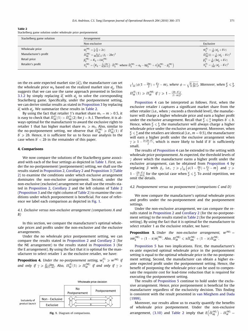
Table 2Stackelberg game solution under wholesale price postponement.

Stackelberg game solution Arrangement

Non-exclusive Exclusive

Wholesale price ~wðNEÞj ¼ 1

4 ðbj

b þ 2cÞ ~wðEÞij ¼ 12b0ða0ij þ b0cÞ

Manufacturer’s profit ~PðNEÞMj ¼

bþd8bð2bþdÞ ðbj � 2bcÞ2 ~PðEÞMj ðiÞ ¼

18b0ða0ij � b0cÞ2

Retail price ~pðNEÞij ¼ Kij þ L ~wðNEÞ

j~pðEÞij ¼

14b0ð3a0ij þ b0cÞ

Retailer’s profit ~pðNEÞij ¼ Kij �

bjþ2bc4ð2bþdÞ

� �� eDðNEÞ

ij where eDðNEÞij ¼ aij � b~pðNEÞ

ij þ d ~pðNEÞkj � ~pðNEÞ

ij

� �~pðEÞij ¼

116b0ða0ij � b0cÞ2

D.A. Andritsos, C.S. Tang / European Journal of Operational Research 204 (2010) 366–375 371

on the ex-ante expected market size (a0i), the manufacturer can setthe wholesale price wij based on the realized market size a0ij. Thissuggests that we can use the same approach presented in Section3.1.2 by simply replacing a0i with a0ij to solve the correspondingStackelberg game. Specifically, under the postponement setting,we can derive similar results as stated in Proposition 3 by replacinga0i with a0ij. We summarize these results in Table 2.

By using the fact that retailer 1’s market share m1 ¼ m > 0:5, itis easy to check that ~PðEÞMj ð1Þ > ~PðEÞMj ð2Þ for j ¼ h; l. Therefore, it is al-ways optimal for the manufacturer to award the exclusive rights toretailer 1 that has higher market share m1 P m2. Also, similar tothe no-postponement setting, we observe that ~PðNEÞ

Mj P ~PðEÞMj ð1Þ ifb0 P 2b. Hence, it is sufficient for us to focus our analysis to thecase when b0 < 2b in the remainder of this paper.

4. Comparisons

We now compare the solutions of the Stackelberg game associ-ated with each of the four settings as depicted in Table 1. First, un-der the no-postponement (postponement) setting, we shall use theresults stated in Proposition 2, Corollary 2 and Proposition 3 (Table2) to examine the conditions under which exclusive arrangementdominates the non-exclusive arrangement. Second, under thenon-exclusive (exclusive) arrangement we shall use the results sta-ted in Proposition 2, Corollary 2 and the left column of Table 2(Proposition 3 and the right column of Table 2) to examine the con-ditions under which postponement is beneficial. For ease of refer-ence we label each comparison as depicted in Fig. 1.

4.1. Exclusive versus non-exclusive arrangement (comparisons A andB)

In this section, we compare the manufacturer’s optimal whole-sale prices and profits under the non-exclusive and the exclusivearrangements.

Under the no wholesale price postponement setting, we cancompare the results stated in Proposition 2 and Corollary 2 (forthe NE arrangement) to the results stated in Proposition 3 (forthe E arrangement). By using the fact that it is optimal for the man-ufacturer to select retailer 1 as the exclusive retailer, we have:

Proposition 4. Under the no-postponement setting, wðEÞ1 P wðNEÞ if

and only if c P b0�2bm2bð1�mÞ. Also, PðEÞM ð1ÞP PðNEÞ

M if and only if c P

Fig. 1. Diagram of comparisons.

11�m ð/ð1� 2bc

bÞ þ b0c

b�mÞ, where / ¼

ffiffiffiffiffiffiffiffiffiffiffiffib0

bbþd

2bþd

q. Moreover, when b0

a0 6ba,

PðEÞM ð1ÞP PðNEÞM if c P 1� ð2b�b0Þc

ð1�mÞb.

Proposition 4 can be interpreted as follows. First, when theexclusive retailer i captures a significant market share from theother retailer (i.e., when c exceeds a threshold level), the manufac-turer will charge a higher wholesale price and earn a higher profitunder the exclusive arrangement. Recall that b0

a0 6ba implies b0 6 b.

Hence, when b0

a0 6ba, the manufacturer will always charge a higher

wholesale price under the exclusive arrangement. Moreover, whenb0

a0 6ba and the retailers are identical (i.e., m ¼ 0:5), the manufacturer

will earn a higher profit under the exclusive arrangement whenc P 1� 2cð2b�b0 Þ

b, which is more likely to hold if b0 is sufficiently

small.The results of Proposition 4 can be extended to the setting with

wholesale price postponement. As expected, the threshold levels ofc above which the manufacturer earns a higher profit under theexclusive arrangement, can be obtained from Proposition 4 byreplacing b with bj, i.e., c P 1

1�m /ð1� 2bcbjÞ þ b0c

bj�m

� �and c P

1� ð2b�b0 Þcð1�mÞbj

for the special case when b0

a0 6ba. To avoid repetition, we

omit the details.

4.2. Postponement versus no postponement (comparisons C and D)

We now compare the manufacturer’s optimal wholesale pricesand profits under the no-postponement and the postponementsettings.

Under the non-exclusive arrangement, we can compare the re-sults stated in Proposition 2 and Corollary 2 (for the no-postpone-ment setting) to the results stated in Table 2 (for the postponementsetting). By using the fact that it is optimal for the manufacturer toselect retailer 1 as the exclusive retailer, we have:

Proposition 5. Under the non-exclusive arrangement, wðNEÞ ¼a~wðNEÞ

h þ ð1� aÞ~wðNEÞl . Also, PðNEÞ

M 6 a ~PðNEÞMh þ ð1� aÞ ~PðNEÞ

Ml .

Proposition 5 has two implications. First, the manufacturer’sex-ante expected optimal wholesale price in the postponementsetting is equal to the optimal wholesale price in the no-postpone-ment setting. Second, the manufacturer can obtain a higher ex-ante expected profit under the postponement setting. Hence, thebenefit of postponing the wholesale price can be used to compen-sate the requisite cost for lead-time reduction that is required forexecuting the postponement setting.

The results of Proposition 5 continue to hold under the exclu-sive arrangement. Hence, price postponement is beneficial for themanufacturer regardless of the exclusivity decision. This findingis consistent with the result presented in van Mieghem and Dada(1999).

Moreover, our results allow us to exactly quantify the benefitsof wholesale price postponement. Under the non-exclusive

arrangement, (3.10) and Table 2 imply that E ~PðNEÞMj

� ��PðNEÞ

M ¼

372 D.A. Andritsos, C.S. Tang / European Journal of Operational Research 204 (2010) 366–375

bþd8bð2bþdÞ ðaðbh � 2bcÞ2 þ ð1�aÞðbl � 2bcÞ2 � ðabh þð1� aÞbl �2bcÞ2Þ ¼

bþd8bð2bþdÞVarðB� 2bcÞ ¼ bþd

8bð2bþdÞVarðBÞ, where Eð�Þ denotes expectation

and Varð�Þ denotes variance. Similarly, under the exclusive arrange-

ment, (3.17) and Table 2 imply that E ~PðEÞMj ð1Þ� �

�PðEÞM ð1Þ ¼ðmþcð1�mÞÞ2

8b0VarðBÞ. Therefore, the benefit of price postponement in-

creases in the variance of the market size, i.e., VarðBÞ. Hence, asthe market condition is more uncertain, the manufacturer shouldconsider postponing his wholesale price decision.

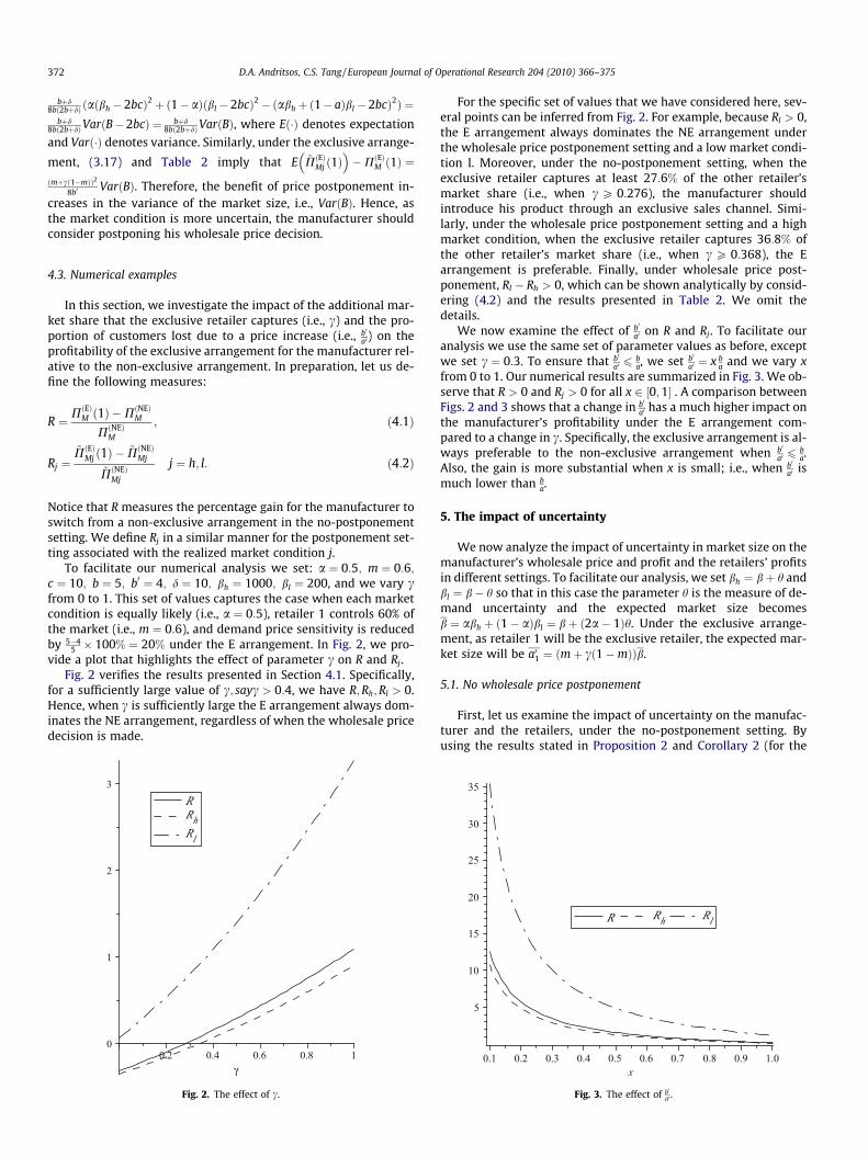
4.3. Numerical examples

In this section, we investigate the impact of the additional mar-ket share that the exclusive retailer captures (i.e., c) and the pro-portion of customers lost due to a price increase (i.e., b0

a0) on theprofitability of the exclusive arrangement for the manufacturer rel-ative to the non-exclusive arrangement. In preparation, let us de-fine the following measures:

R ¼ PðEÞM ð1Þ �PðNEÞM

PðNEÞM

; ð4:1Þ

Rj ¼~PðEÞMj ð1Þ � ~PðNEÞ

Mj

~PðNEÞMj

j ¼ h; l: ð4:2Þ

Notice that R measures the percentage gain for the manufacturer toswitch from a non-exclusive arrangement in the no-postponementsetting. We define Rj in a similar manner for the postponement set-ting associated with the realized market condition j.

To facilitate our numerical analysis we set: a ¼ 0:5; m ¼ 0:6;c ¼ 10; b ¼ 5; b0 ¼ 4; d ¼ 10; bh ¼ 1000; bl ¼ 200, and we vary cfrom 0 to 1. This set of values captures the case when each marketcondition is equally likely (i.e., a ¼ 0:5), retailer 1 controls 60% ofthe market (i.e., m ¼ 0:6), and demand price sensitivity is reducedby 5�4

5 � 100% ¼ 20% under the E arrangement. In Fig. 2, we pro-vide a plot that highlights the effect of parameter c on R and Rj.

Fig. 2 verifies the results presented in Section 4.1. Specifically,for a sufficiently large value of c; sayc > 0:4, we have R;Rh;Rl > 0.Hence, when c is sufficiently large the E arrangement always dom-inates the NE arrangement, regardless of when the wholesale pricedecision is made.

Fig. 2. The effect of c.

For the specific set of values that we have considered here, sev-eral points can be inferred from Fig. 2. For example, because Rl > 0,the E arrangement always dominates the NE arrangement underthe wholesale price postponement setting and a low market condi-tion l. Moreover, under the no-postponement setting, when theexclusive retailer captures at least 27:6% of the other retailer’smarket share (i.e., when c P 0:276), the manufacturer shouldintroduce his product through an exclusive sales channel. Simi-larly, under the wholesale price postponement setting and a highmarket condition, when the exclusive retailer captures 36:8% ofthe other retailer’s market share (i.e., when c P 0:368), the Earrangement is preferable. Finally, under wholesale price post-ponement, Rl � Rh > 0, which can be shown analytically by consid-ering (4.2) and the results presented in Table 2. We omit thedetails.

We now examine the effect of b0

a0 on R and Rj. To facilitate ouranalysis we use the same set of parameter values as before, exceptwe set c ¼ 0:3. To ensure that b0

a0 6ba, we set b0

a0 ¼ x ba and we vary x

from 0 to 1. Our numerical results are summarized in Fig. 3. We ob-serve that R > 0 and Rj > 0 for all x 2 ½0;1� . A comparison betweenFigs. 2 and 3 shows that a change in b0

a0 has a much higher impact onthe manufacturer’s profitability under the E arrangement com-pared to a change in c. Specifically, the exclusive arrangement is al-ways preferable to the non-exclusive arrangement when b0

a0 6ba.

Also, the gain is more substantial when x is small; i.e., when b0

a0 ismuch lower than b

a.

5. The impact of uncertainty

We now analyze the impact of uncertainty in market size on themanufacturer’s wholesale price and profit and the retailers’ profitsin different settings. To facilitate our analysis, we set bh ¼ bþ h andbl ¼ b� h so that in this case the parameter h is the measure of de-mand uncertainty and the expected market size becomesb ¼ abh þ ð1� aÞbl ¼ bþ ð2a� 1Þh. Under the exclusive arrange-ment, as retailer 1 will be the exclusive retailer, the expected mar-ket size will be a01 ¼ ðmþ cð1�mÞÞb.

5.1. No wholesale price postponement

First, let us examine the impact of uncertainty on the manufac-turer and the retailers, under the no-postponement setting. Byusing the results stated in Proposition 2 and Corollary 2 (for the

Fig. 3. The effect of b0

a0 .

Fig. 4. The effect of a.

D.A. Andritsos, C.S. Tang / European Journal of Operational Research 204 (2010) 366–375 373

NE arrangement), the results stated in Proposition 3 (for the Earrangement), and the fact that retailer 1 is awarded the exclusiverights under the E arrangement, we have:

Proposition 6. For any fixed value of h, the manufacturer’s optimalwholesale prices wðNEÞ and wðEÞ1 and the manufacturer’s optimal profitsPðNEÞ

M and PðEÞM ð1Þ under the NE and E arrangements are increasing ina. For any fixed value of a, the manufacturer’s optimal wholesale pricewðNEÞ and wðEÞ1 and the manufacturer’s optimal profit PðNEÞ

M andPðEÞM ð1Þ are decreasing in h when a 2 ½0; 1

2Þ and are increasing in hwhen a 2 ð12 ;1�.

Proposition 6 suggests that, as the probability of having a high’market condition increases (i.e., as a increases), it is optimal for themanufacturer to charge a higher wholesale price and achieve ahigher profit regardless of the exclusivity arrangement. Next, asthe probability of having a ‘high’ market condition a > 0:5, the con-ditional expected market size is higher under condition h(i.e.,abh > ð1� aÞblÞ and the expected market size b ¼ abh þ ð1�aÞbl ¼ bþ ð2a� 1Þh is increasing in the market uncertaintyh. Therefore, the manufacturer can obtain a higher profit as themarket uncertainty h increases under both the NE and E arrange-ments when a > 0:5. Similar reasoning leads to our result whena < 0:5.

By using the results stated in Proposition 2 and Corollary 2 (forthe NE arrangement), the results stated in Proposition 3 (for the Earrangement) and the fact that retailer 1 is awarded the exclusiverights under the E arrangement, we analyze the impact of uncer-tainty on the retailer(s) under the no-postponement setting andget:

Proposition 7. For any fixed value of h, the retail prices pðNEÞij ; i

¼ 1;2, and pðEÞ1j are increasing in a, while the optimal profits pðNEÞij ; i

¼ 1;2, and pðEÞ1j are decreasing in a. Under the exclusive arrangement,

the optimal retail price pðEÞ1h and the optimal profit pðEÞ1h are increasing

in h, while pðEÞ1l and pðEÞ1l are decreasing in h.

By examining the results stated in Propositions 6 and 7, a hasthe same effects on the retailer’s retail price and the manufac-turer’s wholesale price; however, it has the opposite effect on theretailer’s profit and the manufacturer’s profit. This result can be ex-plained as follows: Observe from Propositions 1 and 2 that, under

the NE arrangement, dwðNEÞ

da ¼bh�bl

4b anddpðNEÞ

ij

da ¼ L bh�bl4b . Since

L < 1;dpðNEÞ

ij

da < dwðNEÞ

da . Similarly, it can also be checked thatdpðEÞ

ij

da < dwðEÞ

da . Intuitively, these results imply that as the high marketcondition becomes more likely (i.e., as a increases), the wholesaleprice increases at a faster rate than the retail price. Hence, the re-tailer’s profit reduces as a increases. As such, the manufacturer en-joys a higher profit while the retailer suffers from a lower profit asa increases.

5.2. With wholesale price postponement

In this section, we examine the impact of uncertainty on themanufacturer and the retailers under the postponement setting.From Table 2 we see that no equilibrium quantity depends on asince all decisions are made after the realization of the market con-dition. Therefore, in this section we only consider the effect of h, orequivalently the effect of changes on the realized market size forboth possible market conditions. Using the fact that retailer 1 willbe awarded the exclusive rights under the E arrangement, we sum-marize our results in the following proposition:

Proposition 8. Under the NE and E arrangements, the manufacturer’s

optimal wholesale prices ~wðNEÞj ; ~wðEÞ1j and profits ~PðNEÞ

Mj ; ~PðEÞMj ð1Þ and

the optimal retail prices ~pðNEÞij ; i ¼ 1;2, and ~pðEÞ1j are increasing in h for

j ¼ h and decreasing in h for j ¼ l. Under the E arrangement, retailer

1’s optimal profits ~pðEÞ1j are increasing in h for j ¼ h and decreasing in h

for j ¼ l. Under the NE arrangement, ~pðNEÞ1j is always increasing in h for

j ¼ h and decreasing in h for j ¼ l. When m2 ¼ 1�m P 0:25, ~pðNEÞ2j is

increasing in h for j ¼ h and decreasing in h for j ¼ l.

Note that an increase in h implies an increase in bh and a de-crease in bl. Hence, the above results imply that under the highmarket condition, j ¼ h: as the realized market size bh increases,the manufacturer’s wholesale price and profits and the retailersprices also increase. Retailer 1’s profit exhibits the same behaviorand so does retailer 2’s profit assuming that his market share isabove 0.25. When considering the low market condition the behav-ior of the equilibrium quantities is reversed.

5.3. Numerical examples

In the current section, we investigate the impact of a and h on Rand Rj defined in (4.1) and (4.2), respectively. To examine the effectof a, let us observe from Table 2 that Rj is independent of a. Hence,it suffices to consider R. In our example, we set b ¼ 600; h ¼200; m ¼ 0:6; c ¼ 10; b ¼ 5; b0 ¼ 4; d ¼ 10. These values implythat bh ¼ 800 and bl ¼ 400. In Fig. 4 we plot R as a function ofa 2 ½0;1�. Our plot indicates that as the high market condition be-comes more likely (i.e., as a increases), the benefit of an exclusivearrangement for the manufacturer is reduced. This result can beverified analytically for the case when b0

a0 6ba (which implies

b0 6 b) by observing that dRda ¼ �

2ncðyb�b0cÞðbh�blÞð2yb�b0 Þðb�2bcÞ3

< 0 where

n ¼ bð2bþdÞb0 ðbþdÞ and y ¼ mþ cð1�mÞ. However, if 2yb� b0 < 0 then

dRda > 0 and as the high market condition becomes more likely, thebenefit of an exclusive arrangement increases.

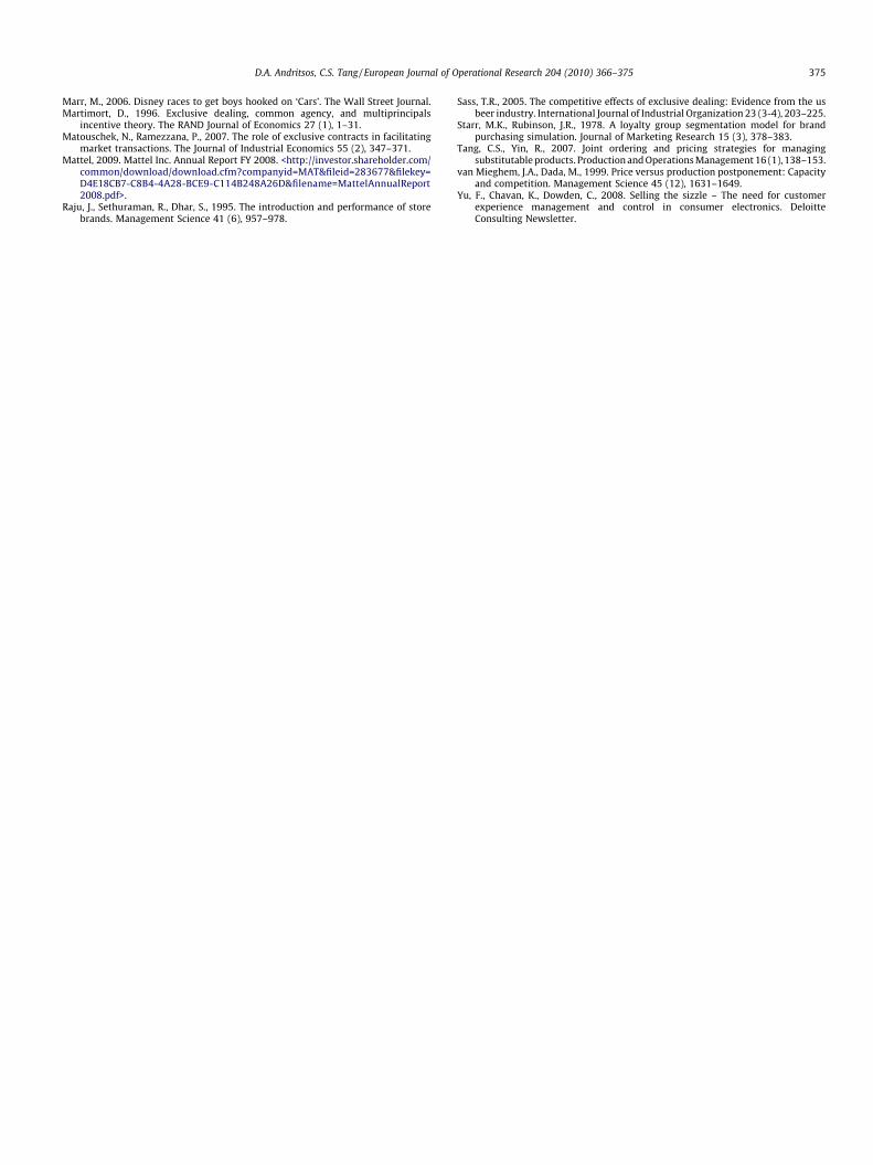
We now turn our attention to examining the effect of h. By usingthe same set of values as above and by considering the case wheneach market condition is equally likely (i.e., a ¼ 0:5), we obtain theplots as depicted in Fig. 5. A change in h has the same impact onboth bh and bl and since a ¼ 0:5, the expected market size b ¼abh þ ð1� aÞbl ¼ b is independent of h and the same is true for

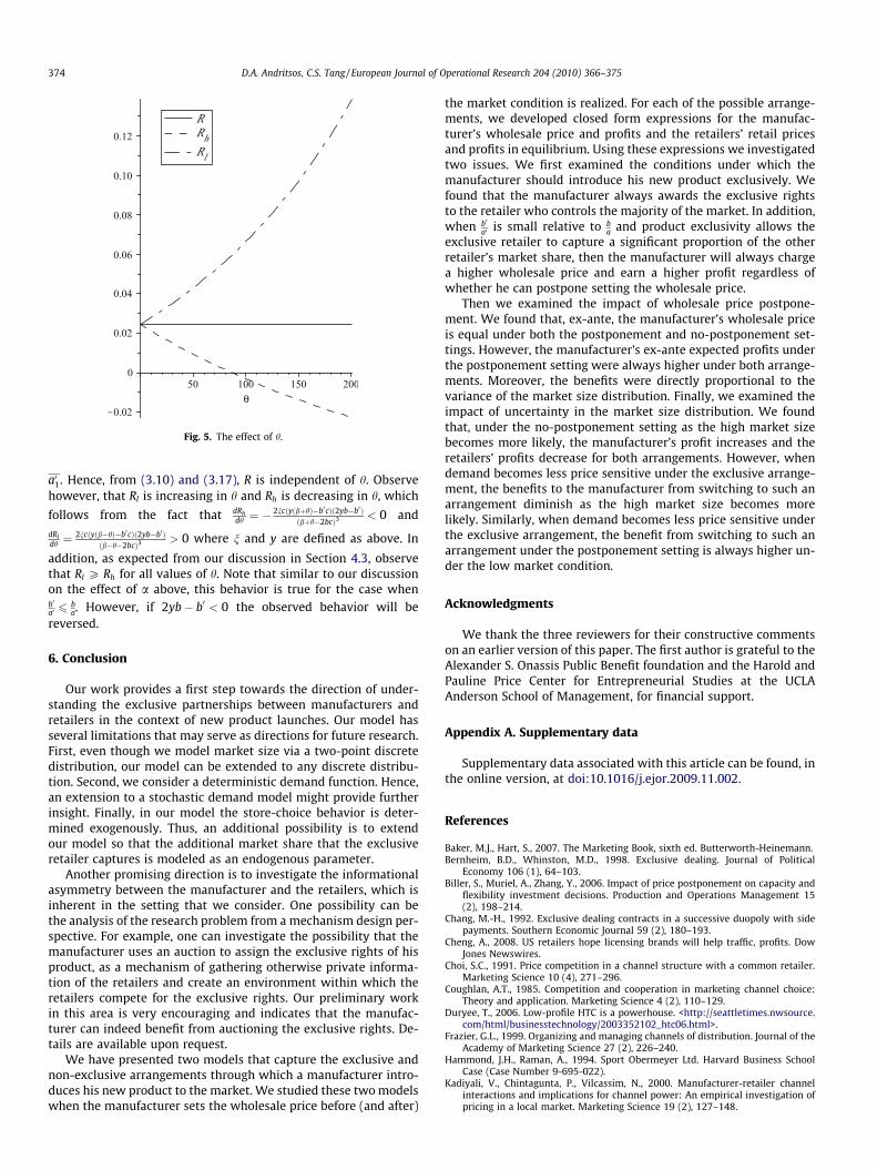
Fig. 5. The effect of h.

374 D.A. Andritsos, C.S. Tang / European Journal of Operational Research 204 (2010) 366–375

a01. Hence, from (3.10) and (3.17), R is independent of h. Observehowever, that Rl is increasing in h and Rh is decreasing in h, which

follows from the fact that dRhdh ¼ �

2ncðyðbþhÞ�b0cÞð2yb�b0 Þðbþh�2bcÞ3

< 0 anddRldh ¼

2ncðyðb�hÞ�b0cÞð2yb�b0 Þðb�h�2bcÞ3

> 0 where n and y are defined as above. In

addition, as expected from our discussion in Section 4.3, observethat Rl P Rh for all values of h. Note that similar to our discussionon the effect of a above, this behavior is true for the case whenb0

a0 6ba. However, if 2yb� b0 < 0 the observed behavior will be

reversed.

6. Conclusion

Our work provides a first step towards the direction of under-standing the exclusive partnerships between manufacturers andretailers in the context of new product launches. Our model hasseveral limitations that may serve as directions for future research.First, even though we model market size via a two-point discretedistribution, our model can be extended to any discrete distribu-tion. Second, we consider a deterministic demand function. Hence,an extension to a stochastic demand model might provide furtherinsight. Finally, in our model the store-choice behavior is deter-mined exogenously. Thus, an additional possibility is to extendour model so that the additional market share that the exclusiveretailer captures is modeled as an endogenous parameter.

Another promising direction is to investigate the informationalasymmetry between the manufacturer and the retailers, which isinherent in the setting that we consider. One possibility can bethe analysis of the research problem from a mechanism design per-spective. For example, one can investigate the possibility that themanufacturer uses an auction to assign the exclusive rights of hisproduct, as a mechanism of gathering otherwise private informa-tion of the retailers and create an environment within which theretailers compete for the exclusive rights. Our preliminary workin this area is very encouraging and indicates that the manufac-turer can indeed benefit from auctioning the exclusive rights. De-tails are available upon request.

We have presented two models that capture the exclusive andnon-exclusive arrangements through which a manufacturer intro-duces his new product to the market. We studied these two modelswhen the manufacturer sets the wholesale price before (and after)

the market condition is realized. For each of the possible arrange-ments, we developed closed form expressions for the manufac-turer’s wholesale price and profits and the retailers’ retail pricesand profits in equilibrium. Using these expressions we investigatedtwo issues. We first examined the conditions under which themanufacturer should introduce his new product exclusively. Wefound that the manufacturer always awards the exclusive rightsto the retailer who controls the majority of the market. In addition,when b0

a0 is small relative to ba and product exclusivity allows the

exclusive retailer to capture a significant proportion of the otherretailer’s market share, then the manufacturer will always chargea higher wholesale price and earn a higher profit regardless ofwhether he can postpone setting the wholesale price.

Then we examined the impact of wholesale price postpone-ment. We found that, ex-ante, the manufacturer’s wholesale priceis equal under both the postponement and no-postponement set-tings. However, the manufacturer’s ex-ante expected profits underthe postponement setting were always higher under both arrange-ments. Moreover, the benefits were directly proportional to thevariance of the market size distribution. Finally, we examined theimpact of uncertainty in the market size distribution. We foundthat, under the no-postponement setting as the high market sizebecomes more likely, the manufacturer’s profit increases and theretailers’ profits decrease for both arrangements. However, whendemand becomes less price sensitive under the exclusive arrange-ment, the benefits to the manufacturer from switching to such anarrangement diminish as the high market size becomes morelikely. Similarly, when demand becomes less price sensitive underthe exclusive arrangement, the benefit from switching to such anarrangement under the postponement setting is always higher un-der the low market condition.

Acknowledgments

We thank the three reviewers for their constructive commentson an earlier version of this paper. The first author is grateful to theAlexander S. Onassis Public Benefit foundation and the Harold andPauline Price Center for Entrepreneurial Studies at the UCLAAnderson School of Management, for financial support.

Appendix A. Supplementary data

Supplementary data associated with this article can be found, inthe online version, at doi:10.1016/j.ejor.2009.11.002.

References

Baker, M.J., Hart, S., 2007. The Marketing Book, sixth ed. Butterworth-Heinemann.Bernheim, B.D., Whinston, M.D., 1998. Exclusive dealing. Journal of Political

Economy 106 (1), 64–103.Biller, S., Muriel, A., Zhang, Y., 2006. Impact of price postponement on capacity and

flexibility investment decisions. Production and Operations Management 15(2), 198–214.

Chang, M.-H., 1992. Exclusive dealing contracts in a successive duopoly with sidepayments. Southern Economic Journal 59 (2), 180–193.

Cheng, A., 2008. US retailers hope licensing brands will help traffic, profits. DowJones Newswires.

Choi, S.C., 1991. Price competition in a channel structure with a common retailer.Marketing Science 10 (4), 271–296.

Coughlan, A.T., 1985. Competition and cooperation in marketing channel choice:Theory and application. Marketing Science 4 (2), 110–129.

Duryee, T., 2006. Low-profile HTC is a powerhouse. <http://seattletimes.nwsource.com/html/businesstechnology/2003352102_htc06.html>.

Frazier, G.L., 1999. Organizing and managing channels of distribution. Journal of theAcademy of Marketing Science 27 (2), 226–240.

Hammond, J.H., Raman, A., 1994. Sport Obermeyer Ltd. Harvard Business SchoolCase (Case Number 9-695-022).

Kadiyali, V., Chintagunta, P., Vilcassim, N., 2000. Manufacturer-retailer channelinteractions and implications for channel power: An empirical investigation ofpricing in a local market. Marketing Science 19 (2), 127–148.

D.A. Andritsos, C.S. Tang / European Journal of Operational Research 204 (2010) 366–375 375

Marr, M., 2006. Disney races to get boys hooked on ‘Cars’. The Wall Street Journal.Martimort, D., 1996. Exclusive dealing, common agency, and multiprincipals

incentive theory. The RAND Journal of Economics 27 (1), 1–31.Matouschek, N., Ramezzana, P., 2007. The role of exclusive contracts in facilitating

market transactions. The Journal of Industrial Economics 55 (2), 347–371.Mattel, 2009. Mattel Inc. Annual Report FY 2008. <http://investor.shareholder.com/

common/download/download.cfm?companyid=MAT&fileid=283677&filekey=D4E18CB7-C8B4-4A28-BCE9-C114B248A26D&filename=MattelAnnualReport2008.pdf>.

Raju, J., Sethuraman, R., Dhar, S., 1995. The introduction and performance of storebrands. Management Science 41 (6), 957–978.

Sass, T.R., 2005. The competitive effects of exclusive dealing: Evidence from the usbeer industry. International Journal of Industrial Organization 23 (3-4), 203–225.

Starr, M.K., Rubinson, J.R., 1978. A loyalty group segmentation model for brandpurchasing simulation. Journal of Marketing Research 15 (3), 378–383.

Tang, C.S., Yin, R., 2007. Joint ordering and pricing strategies for managingsubstitutable products. Production and Operations Management 16 (1), 138–153.

van Mieghem, J.A., Dada, M., 1999. Price versus production postponement: Capacityand competition. Management Science 45 (12), 1631–1649.

Yu, F., Chavan, K., Dowden, C., 2008. Selling the sizzle – The need for customerexperience management and control in consumer electronics. DeloitteConsulting Newsletter.