Embed Size (px)
Citation preview

Bull Math Biol (2011) 73:2013–2044DOI 10.1007/s11538-010-9597-1
O R I G I NA L A RT I C L E
Law of the Minimum Paradoxes
Alexander N. Gorban · Lyudmila I. Pokidysheva ·Elena V. Smirnova · Tatiana A. Tyukina
Received: 10 July 2009 / Accepted: 18 October 2010 / Published online: 19 November 2010© Society for Mathematical Biology 2010
Abstract The “Law of the Minimum” states that growth is controlled by the scarcestresource (limiting factor). This concept was originally applied to plant or crop growth(Justus von Liebig, 1840, Salisbury, Plant physiology, 4th edn., Wadsworth, Bel-mont, 1992) and quantitatively supported by many experiments. Some generaliza-tions based on more complicated “dose-response” curves were proposed. Violationsof this law in natural and experimental ecosystems were also reported. We studymodels of adaptation in ensembles of similar organisms under load of environmentalfactors and prove that violation of Liebig’s law follows from adaptation effects. If thefitness of an organism in a fixed environment satisfies the Law of the Minimum thenadaptation equalizes the pressure of essential factors and, therefore, acts against theLiebig’s law. This is the the Law of the Minimum paradox: if for a randomly cho-sen pair “organism–environment” the Law of the Minimum typically holds, then in awell-adapted system, we have to expect violations of this law.
For the opposite interaction of factors (a synergistic system of factors which am-plify each other), adaptation leads from factor equivalence to limitations by a smallernumber of factors.
For analysis of adaptation, we develop a system of models based on Selye’s ideaof the universal adaptation resource (adaptation energy). These models predict thatunder the load of an environmental factor a population separates into two groups(phases): a less correlated, well adapted group and a highly correlated group witha larger variance of attributes, which experiences problems with adaptation. Some
A.N. Gorban (�) · T.A. TyukinaCentre for Mathematical Modelling, University of Leicester, Leicester, LE1 7RH, UKe-mail: [email protected]
T.A. Tyukinae-mail: [email protected]
L.I. Pokidysheva · E.V. SmirnovaSiberian Federal University, Krasnoyarsk, 660041, Russia

2014 A.N. Gorban et al.
empirical data are presented and evidences of interdisciplinary applications to econo-metrics are discussed.
Keywords Liebig’s Law · Adaptation · Fitness · Stress
1 Introduction
1.1 The Law of the Minimum
The “Law of the Minimum” states that growth is controlled by the scarcest resource(limiting factor) (Salisbury 1992). This law is usually believed to be the result ofJustus von Liebig’s research (1840) but the agronomist and chemist Carl Sprengelpublished in 1828 an article that contained in essence the Law of the Minimum andthis law can be called the Sprengel–Liebig Law of the Minimum (van der Ploeg et al.1999).
This concept is illustrated in Fig. 1.This concept was originally applied to plant or crop growth. Many times it was
criticized, rejected, and then returned to and demonstrated quantitative agreementwith experiments (Salisbury 1992; Paris 1992; Cade et al. 1999).
The Law of the Minimum was extended to a more general conception of factors,rather than for the elementary physical description of available chemical substancesand energy. Any environmental factor essential for life that is below the critical min-imum, or that exceeds the maximum tolerable level could be considered as a limitingone.
There were several attempts to create a general theory of factors and limitation inecology, physiology, and evolutionary biology. Tilman (1980) proposed an equilib-rium theory of resource competition based on classification of interaction in pairs ofresources. They may be: (1) essential, (2) hemi-essential, (3) complementary, (4) per-fectly substitutable, (5) antagonistic, or (6) switching. This interaction depends onspatial heterogeneity of resource distributions. For various resource types, the gen-eral criterion for stable coexistence of species was developed.
Fig. 1 The Law of the Minimum. Coordinates c1, c2 are normalized values of factors. For a given states = (c1(s), c2(s)), the bold solid line min{c1, c2} = min{c1(s), c2(s)} separates the states with better con-ditions (higher productivity) from the states with worse conditions. On this line, the conditions do notdiffer significantly from s because of the same value of the limiting factor. The dot dash line shows theborder of survival. On the dashed line, the factors are equally important (c1 = c2)

Law of the Minimum Paradoxes 2015
Bloom et al. (1985), Chapin (1990) elaborated the economical metaphor of eco-logical concurrency. This analogy allowed them to merge the optimality and the lim-iting approach and to formulate four “theorems.” In particular, Theorem 3 states thata plant should adjust allocation so that, for a given expenditure in acquiring eachresource, it achieves the same growth response: growth is equally limited by all re-sources. This is a result of adjustment: adaptation makes the limiting factors equallyimportant. They also studied the possibility for resources to substitute for one another(Theorem 4) and introduced the concept of “exchange rate.”
For human physiology, the observation that adaptation makes the limiting factorsequally important was supported by many data of human adaptation to the Far Northconditions (or which is the same, disadaptation causes inequality of factors and leadsto appearance of single limiting factor) (Gorban et al. 1987). The theory of factors—resource interaction was developed and supported by experimental data. The resultsare used for monitoring of human populations in Far North (Sedov et al. 1988).
In their perspectives paper, Sih and Gleeson (1995) considered three inter-relatedissues which form the core of evolutionary ecology: (1) key environmental factors;(2) organismal traits that are responses to the key factors; (3) the evolution of thesekey traits. They suggested to focus on “limiting traits” rather than optimal traits.Adaptation leads to optimality and equality of traits as well as of factors but undervariations some traits should be more limiting than others. From the Sih and Gleesonpoint of view, there is a growing awareness of the potential value of the limiting traitsapproach as a guide for studies in both basic and applied ecology.
The critics of the Law of the Minimum is usually based on the “colimitation” phe-nomenon: limitation of growth and survival by a group of equally important factorsand traits. For example, analysis of species-specific growth and mortality of juveniletrees at several contrasting sites suggests that light and other resources can be simul-taneously limiting, and challenges the application of the Law of the Minimum to treesapling growth (Kobe 1996).
The concept of multiple limitation was proposed for unicellular organisms basedon the idea of the nutritional status of an organism expressed in terms of state vari-ables (van den Berg 1998). The property of being limiting was defined in terms of thereserve surplus variables. This approach was illustrated by numerical experiments.
In the world oceans, there are high nutrient-low chlorophyll regions where chloro-phyll concentrations are lower than expected concentrations given the ambient phos-phate and nitrate levels. In these regions, limitations of phytoplankton growth byother nutrients like silicate or iron have been hypothesized and supported by experi-ments. This colimitation was studied using a nine-component ecosystem model em-bedded in the HAMOCC5 model of the oceanic carbon cycle (Aumont et al. 2003).
The double-nutrient-limited growth appears also as a transition regime betweentwo regimes with single limiting factor. For bacteria and yeasts at a constant dilutionrate in the chemostat, three distinct growth regimes were recognized: (1) a clearlycarbon-limited regime with the nitrogen source in excess, (2) a double-nutrient-limited growth regime where both the carbon and the nitrogen source were belowthe detection limit, and (3) a clearly nitrogen-limited growth regime with the carbonsource in excess. The position of the double-nutrient-limited zone is very narrow athigh growth rates and becomes broader during slow growth (Egli and Zinn 2003;Zinn et al. 2004).

2016 A.N. Gorban et al.
Decomposition of soil organic matter is limited by both the available substrate andthe active decomposer community. The colimitation effects strongly affect the feed-backs of soil carbon to global warming and its consequences (Wutzler and Reichstein2008).
Dynamics of communities lead to colimitation on community level even if or-ganisms and populations remain limited by single factors. Communities are likely toadjust their stoichiometry by competitive exclusion and coexistence mechanisms. Itguarantees simultaneous limitation by many resources and optimal use of them at thecommunity scale. This conclusion was supported by a simple resource ratio modeland an experimental test carried out in microcosms with bacteria (Danger et al. 2008).
In spite of the long previous discussion of colimitation, in 2008, Saito andGoepfert stressed that this notion is “an important yet often misunderstood concept”(Saito and Goepfert 2008). They describe the potential nutrient colimitation pairs inthe marine environment and define three types of colimitation:
I. Independent nutrient colimitation concerns two elements that are generally bio-chemically mutually exclusive, but are also both found in such low concentra-tions as to be potentially limiting. Example: nitrogen-phosphorus colimitation.
II. Biochemical substitution colimitation involves two elements that can substitutefor the same biochemical role within the organism. Example: zinc–cobalt colim-itation.
III. Biochemically dependent colimitation refers to the limitation of one element thatmanifests itself in an inability to acquire another element. Example: zinc–carboncolimitation.
The experimental colimitation examples of the first type do not refute the Law ofthe Minimum completely but rather support the following statement: the ecologicalsystems of various levels, from an organism to a community, may avoid the mono-limitation regime either by the natural adjustment of their consumption structure(Bloom et al. 1985; Semevsky and Semenov 1982) or just by living in the transi-tion zone between the monolimitation regimes. From the general point of view (Sihand Gleeson 1995), such a transition zone is expected to be quite narrow (as a vicin-ity of a surface where factors are equal) but in some specific situations it may bebroad, for example, for slow growth regimes in the chemostat (Egli and Zinn 2003;Zinn et al. 2004).
The type II and type III colimitations should be carefully separated from the usualdiscussion of the Law of the Minimum limitation. For these types of colimitation, two(or more) nutrients limit growth rates simultaneously, either through the effect of bio-chemical substitution (type II) or by depressing the ability for the uptake of anothernutrient (type III) (Saito and Goepfert 2008). The type II and type III colimitationsgive us examples of the “non-Liebig” organization of the system of factors.
The Law of the Minimum is one of the most important tools for mathematicalmodeling of ecological systems. It gives a clue for constructing the first model formulticomponent and multifactor systems. This clue sounds rather simple: First of all,we have to take into account the most important factors which are probably limitingfactors. Everything else should be excluded and allowed back only in a case when a“sufficient reason” is proved (following the famous “Principle of Sufficient Reason”by Leibnitz, one of the four recognized laws of thought).

Law of the Minimum Paradoxes 2017
It is suggested to consider the Liebig production function as the “archetype” forecological modeling (Nijland et al. 2008). The generalizations of the Law of the Min-imum were supported by the biochemical idea of limiting reaction steps (see, for ex-ample, (Brown and Cooper 1993), or recent review, (Gorban and Radulescu 2008)).Three classical production functions, the Liebig, Mitscherlich, and Liebscher rela-tions between nutrient supply and crop production, are limiting cases of an integratedmodel based on the Michaelis–Menten kinetic equation (Nijland et al. 2008).
Applications of the Law of the Minimum to the ecological modeling are verybroad. The quantitative theories of the bottom–up control of the phytoplanktondynamics is based on the influence of limiting nutrients on growth and repro-duction. The most used is the Droop model and its generalizations (Droop 1973;Legovic and Cruzado 1997; Ballantyne et al. 2008).
The Law of the Minimum was combined with the evolutionary dynamics to ana-lyze the “Paradox of the plankton” (Shoresh et al. 2008) formulated by Hutchinson in1961: “How it is possible for a number of species to coexist in a relatively isotropic orunstructured environment all competing for the same sorts of materials. . . Accordingto the principle of competitive exclusion. . . we should expect that one species alonewould out compete all of the others.” It was shown that evolution exacerbates theparadox and it is now very far from the resolution.
The theory of evolution from monolimitation toward colimitation was developedthat takes into account the viruses attacks on the phytoplankton receptors (Mengeand Weitz 2009). In the classic theory (Tilman 1982), evolution toward colimitationdecreases equilibrium resource concentrations and increases equilibrium populationdensity. In contrary, under influence of viruses, evolution toward colimitation mayhave no effect on equilibrium resource concentrations and may decrease the equilib-rium population density (Menge and Weitz 2009).
The Law of the Minimum was used for modeling of microcolonial fungi growth onrock surfaces (Chertov et al. 2004). The analysis demonstrated that a continued lackof organic nutrition is a dominating environmental factor limiting growth on stonemonuments and other exposed rock surfaces in European temperate and Mediter-ranean climate.
McGill (2005) developed a model of coevolution of mutualisms where one re-source is traded for another resource. The mechanism is based on the Law of theMinimum in combination with Tilman’s approach to resource competition (Tilman1980, 1982). It was shown that resource limitations cause mutualisms to have stablepopulation dynamics.
The Law of the Minimum produces the piecewise linear growth functions whichare nonsmooth and very far from being linear. This nonlinearity transforms normalor uniform distributions of resource availabilities into skewed crop yield distributionand no natural satisfactory motivation exists in favor of any simple crop yield distri-bution (Hennessy 2009). With independent, identical, uniform resource availabilitydistributions the yield skew is positive, and it is negative for normal distributions.
The standard linear tools of statistics such as generalized linear models do notwork satisfactory for systems with limiting factors. Conventional correlation analysisconflicts with the concept of limiting factors. This was demonstrated in a study ofthe spatial distribution of Glacier lily in relation to soil properties and gopher distur-bance (Thomson et al. 1996). For systems with limiting factors, quantile regression
2018 A.N. Gorban et al.
performs much better with strong theoretical justification in Law of the Minimum(Austin 2007).
Some of the generalizations of the Law of the Minimum went quite far from agri-culture and ecology. The Law of the Minimum was applied to economics (Daly 1991)and to education, for example, Ozden (2004).
Recently, a strong mathematical background was created for the Law of the Min-imum. Now the limiting factors theory together with static and dynamic limitationin chemical kinetics (Gorban and Radulescu 2008; Gorban et al. 2010) are consid-ered as the realization of the Maslov dequantization (Kolokoltsov and Maslov 1997;Litvinov and Maslov 2005; Litvinov 2007) and idempotent analysis. Roughly speak-ing, the limiting factor formalism means that we should handle any two quantitiesc1, c2 either as equal numbers or as numbers connected by the relation �: eitherc1 � c2 or c1 � c2. Such a hard nonlinearity can arise in the smooth dynamic mod-els because of the time-scale separation (van den Berg 1998).
Dequantization of the traditional mathematics leads to a mathematics over tropicalalgebras like the max-plus algebra. Since the classical work of Kleene (1956), thesealgebras are intensively used in mathematics and computer science, and the con-cept of dequantization and idempotent analysis opened new applications in physicsand other natural sciences (see the comprehensive introduction in Litvinov 2007).Liebig’s and anti-Liebig’s (see Definition 1 below) systems of factors may be consid-ered as realizations of max-plus or min-plus asymptotics correspondingly.
1.2 Fitness Convexity, Concavity and Various Interactions Between Factors
There exist an opposite type of organization of the system of factors, which from afirst glance, seems to be symmetric to Liebig’s type of interaction between them. InLiebig’s systems, the factor with the worst value determines the growth and surviving.The completely opposite situation is: the factor with the best value determines every-thing. We call such a system “anti-Liebig’s” one. Of course, it seems improbable thatall the possible factors interact following the Law of the Minimum or the fully op-posite anti-Liebig’s rule. Interactions between factors in real systems are much morecomplicated (Saito and Goepfert 2008). Nevertheless, we can state a question abouthierarchical decomposition of the system of factors in elementary groups with simpleinteractions inside, then these elementary groups can be clustered into superfactorswith simple interactions between them, and so on.
Let us introduce some notions and notations. We consider organisms that areunder the influence of several factors F1, . . . ,Fq . Each factor has its intensity fi
(i = 1, . . . , q). For convenience, we consider all these factors as negative or harmful.This is just a convention about the choice of axes directions: a wholesome factor isjust a “minus harmful” factor.
At this stage, we do not specify the nature of these factors. Formally, they are justinputs in the adaptation dynamics, the arguments of the fitness functions.
The fitness function is the central notion of the evolutionary and ecological dy-namics. This is a function that maps the environmental factors and traits of theorganism into the reproduction coefficient, that is, its contribution, in offspring toits population. Fisher proposed to construct fitness as a combination of indepen-dent individual contribution of various traits (Fisher 1930). Haldane (1932) criticized

Law of the Minimum Paradoxes 2019
the approach based on independent actions of traits. Modern definitions of fitnessfunction are based on adaptation dynamics. For the structured populations, the fit-ness should be defined through the dominant Lyapunov exponents (Gorban 1984;Metz et al. 1992). In the evolutionary game theory (Maynard-Smith 1982), payoffrepresents Darwinian fitness and describes how the use of the strategy improves ananimal’s prospects for survival and reproduction. Recently, the Fisher and Haldaneapproaches are combined (Waxman and Welch 2005): Haldane’s concern is incor-porated into Fisher’s model by allowing the intensity of selection to vary betweentraits.
It is a nontrivial task to measure the fitness functions and action of selection innature, but now it has been done for many populations and phenotypical traits (King-solver and Pfennig 2007). Special statistical methods for life-history analysis for in-ference of fitness and population growth are developed and tested (Shaw et al. 2008).
In our further analysis, we do not need exact values of fitness but rather its exis-tence and some qualitative features.
First of all, let us consider an oversimplified situation with identical organ-isms. Given phenotypical treats, fitness W is a function of factor loads: W =W(f1, . . . , fq). This assumption does not take into account physiological adaptationthat works as a protection system and modifies the factor loads. This modification isin the focus of our analysis in the follow-up section, but for now we neglect adapta-tion. The convention about axes direction means that all the partial derivatives of W
are nonpositive ∂W/∂fi ≤ 0.By definition, for a Liebig’s system of factors W is a function of the worst (max-
imal) factor intensity: W = W(max{f1, . . . , fq}) (Fig. 2a) and for anti-Liebig’s sys-tem it is the function of the best (minimal) factor intensity W = W(min{f1, . . . , fq})(Fig. 2c). Such representations as well as the usual formulation of the Law of theMinimum require special normalization of factor intensities to compare the loads ofdifferent factors.
Fig. 2 Various types oforganization of the system offactors. For a given state s, thebold solid line is given by theequation W(f1, f2) = W(s).This line separates the area withhigher fitness (“betterconditions”) from the line withlower fitness (“worseconditions”). In Liebig’s (a) andgeneralized Liebig’s systems (b)the area of better conditions isconvex, in “anti-Liebig’s”systems (c) and the generalsynergistic systems (d) the areaof worse conditions is convex.The dot dash line shows theborder of survival. On thedashed line, the factors areequally important (f1 = f2)

2020 A.N. Gorban et al.
Fig. 3 Conditional optimization for various systems of factors. Because of convexity conditions, fitnessachieves its maximum on an interval L for Liebig’s system (a) on the diagonal (the factors are equallyimportant), for generalized Liebig’s systems (b) near the diagonal, for anti-Liebig’s system (c) and for thegeneral synergistic system (d) this maximum is one of the ends of the interval L
For Liebig’s systems of factors, the superlevel sets of W given by inequalitiesW ≥ w0 are convex for any level w0 in a convex domain (Fig. 2a). For anti-Liebig’ssystems of factors, the sublevel sets of W given by inequalities W ≤ w0 are convexfor any level w0 in a convex domain (Fig. 2c).
These convexity properties are essential for optimization problems which arisein the modeling of adaptation and evolution. Let us take them as definitions of thegeneralized Liebig and anti-Liebig systems of factors.
Definition 1
1. A system of factors is the generalized Liebig system in a convex domain U , if forany level w0 the superlevel set {f ∈ U | W(f ) ≥ w0} is convex (Fig. 2b).
2. A system of factors is the generalized anti-Liebig system in a convex domain U ,if for any level w0 the sublevel set {f ∈ U | W(f ) ≤ w0} is convex (Fig. 2d).
We call the generalized anti-Liebig systems of factors the synergistic systems be-cause this formalizes the idea of synergy: in the synergistic systems harmful factorssuperlinear amplify each other.
Conditional maximization of fitness destroys the symmetry between Liebig’s andanti-Liebig’s systems as well as between generalized Liebig’s systems and syner-gistic ones. Following the geometric approach of Tilman (1980, 1982), we illustratethis optimization on Fig. 3. The picture may be quite different from the conditionalmaximization of a convex function near its minima point (compare, for example,Figs. 3c, 3d to Fig. from Sih and Gleeson 1995).

Law of the Minimum Paradoxes 2021
Individual adaptation changes the picture. In the next subsection, we discuss pos-sible mechanism of these changes.
1.3 Adaptation Energy and Factor–Resource Models
The reaction of an organism to the load of a single factor may have plateaus (intervalsof tolerance considered in Shelford’s “law of tolerance,” Odum 1971, Chap. 5). Thedose-response curves may be nonmonotonic (Colborn et al. 1996) or even oscillating.Nevertheless, we start from a very simple abstract model that is close to the usualfactor analysis.
We consider organisms that are under the influence of several harmful factorsF1, . . . ,Fq with intensities fi (i = 1, . . . , q). Each organism has its adaptation sys-tems, a “shield” that can decrease the influence of external factors. In the simplestcase, it means that each system has an available adaptation resource, R, which canbe distributed for the neutralization of factors: instead of factor intensities fi the sys-tem is under pressure from factor values fi − airi (where ai > 0 is the coefficientof efficiency of factor Fi neutralization by the adaptation system and ri is the shareof the adaptation resource assigned for the neutralization of factor Fi ,
∑i ri ≤ R).
The zero value fi − airi = 0 is optimal (the fully compensated factor), and furthercompensation is impossible and senseless.
For unambiguity of terminology, we use the term “factor” for all factors includingany deficit of available external resource or even some illnesses. We keep the term“resource” for internal resources, mostly for the hypothetical Selye’s “adaptation en-ergy.”
It should be specially stressed that the adaptation energy is neither physical energynor a substance. This idealization describes the experimental results: in many exper-iments it was demonstrated that organisms under load of various factors behave as ifthey spend a resource, which is the same for different factors. This resource may beexhausted and then the organism dies.
We represent the organisms, which are adapting to stress, as the systems whichoptimize distribution of available amount of a special adaptation resource for neutral-ization of different aggressive factors (we consider the deficit of anything necessaryas a negative factor, also). These factor–resource models with optimization are veryconvenient for the modeling of adaptation. We use a class of models many factors—one resource.
Interaction of each system with a factor Fi is described by two quantities: thefactor Fi pressure ψi = fi − airi and the resource ri assigned to the factor Fi neu-tralization. The first quantity characterizes how big the uncompensated harm is fromthat factor, the second quantity measures, how intensive is the adaptation answer tothe factor (or how far the system was modified to answer the factor Fi pressure).
Already one factor-one resource models of adaptation produce the tolerance law.We demonstrate below that it predicts the separation of groups of organism intotwo subgroups: the less correlated well-adapted organisms and highly correlatedorganisms with a deficit of the adaptation resource. The variance is also higherin the highly correlated group of organisms with a deficit of the adaptation re-source.

2022 A.N. Gorban et al.
This result has a clear geometric interpretation. Let us represent each organism asa data point in an n-dimensional vector space. Assume that they fall roughly withinan ellipsoid. The well-adapted organisms are not highly correlated and after normal-ization of scales to unit variance the corresponding cloud of points looks roughly as asphere. The organisms with a deficit of the adaptation resource are highly correlated,hence in the same coordinates their cloud looks like an ellipsoid with remarkableeccentricity. Moreover, the largest diameter of this ellipsoid is larger than for thewell-adapted organisms and the variance increases together with the correlations.
This increase of variance together with correlations may seem counterintuitive be-cause it has no formal backgrounds in definitions of the correlation coefficients andvariance. This is an empirical finding that under stress correlations and variance in-crease together, supported by many observations both for physiological and financialsystems. The factor–resource models give a plausible explanation of this phenomena.
The crucial question is: what is the resource of adaptation? This question arosefor the first time when Selye published the concept of adaptation energy and ex-perimental evidence supporting this idea (Selye 1938a, 1938b). Selye found that theorganisms (rats) which demonstrate no differences in normal environment may differsignificantly in adaptation to an increasing load of environmental factors. Moreover,when he repeated the experiments, he found that adaptation ability decreases afterstress. All the observations could be explained by existence of an universal adapta-tion resource that is being spent during all adaptation processes.
Selye’s ideas allow the following interpretation: the aggressive influence of theenvironment on the organism may be represented as an action of independent fac-tors. The system of adaptation consists of subsystems, which protect the organismfrom different factors. These subsystems consume the same resource, the adaptationenergy. The distribution of this resource between the subsystems depends on envi-ronmental conditions.
Later the concept of adaptation energy was significantly improved (Goldstone1952), plenty of indirect evidence supporting this concept were found, but this elu-sive adaptation energy is still a theoretical concept, and in the modern “Encyclopediaof Stress” we read: “As for adaptation energy, Selye was never able to measure it. . .”(McCarty and Pasak 2000). Nevertheless, the notion of adaptation energy is very use-ful in the analysis of adaptation and is now in wide use (see, for example, Breznitz1983; Schkade and Schultz 2003).
The idea of exchange can help in the understanding of adaptation energy: thereare many resources, but any resource can be exchanged for another one. To studysuch an exchange, an analogy with the currency exchange is useful. Following thisanalogy, we have to specify, what is the exchange rate, how fast this exchangecould be done (what is the exchange time), what is the margin, and how the mar-gin depends on the exchange time. There may appear various limitations of theamount of the exchangeable resource, and so on. The economic metaphor for eco-logical concurrency and adaptation was elaborated in 1985 (Bloom et al. 1985;Chapin 1990) but much earlier, in 1952, it was developed for physiological adap-tation (Goldstone 1952).
Market economics seems closer to the idea of resource universalization than biol-ogy is, but for biology this exchange idea also seems useful. Of course, there exist

Law of the Minimum Paradoxes 2023
some limits on the possible exchanges of different resources. It is possible to includethe exchange processes into models, but many questions arise about unknown coef-ficients. Nevertheless, we can follow Selye’s arguments and postulate the adaptationenergy as a universal adaptation resource.
The adaptation energy is neither physical energy nor a substance. This is a the-oretical construction, which may be considered as a pool of various exchangeableresources. When an organism achieves the limits of resource exchangeability, theuniversal nonspecific stress and adaptation syndrome transforms (disintegrates) intospecific diseases. Near this limit, we have to expect the critical retardation (Gorban2004) of exchange processes.
Adaptation optimizes the state of the system for given available amounts of theadaptation resource. This idea seems very natural, but it may be a difficult task tofind the objective function that is hidden behind the adaptation process. Nevertheless,even an assumption about the existence of an objective function and about its generalproperties helps in analysis of adaptation process.
Assume that adaptation should maximize a fitness function W which depends onthe compensated values of factors, ψi = fi − airi for the given amount of availableresource:
⎧⎨
⎩
W(f1 − a1r1, f2 − a2r2, . . . , fq − aqrq) → max;ri ≥ 0, fi − airi ≥ 0,
∑q
i=1 ri ≤ R.(1)
The only question is: How can we be sure that adaptation follows any optimalityprinciple? Existence of optimality is proven for microevolution processes and eco-logical succession. The mathematical backgrounds for the notion of “natural selec-tion” in these situations are well-established after work by Haldane (1932) and Gause(1934). Now this direction with various concepts of fitness (or “generalized fitness”)optimization is elaborated in many details (see, for example, review papers, Bomze2002; Oechssler and Riedel 2002; Gorban 2007).
The foundation of optimization is not so clear for such processes as modificationsof a phenotype, and for adaptation in various time scales. The idea of genocopy-phenocopy interchangeability was formulated long ago by biologists to explain manyexperimental effects: the phenotype modifications simulate the optimal genotype(West-Eberhard 2003, p. 117). The idea of convergence of genetic and environmentaleffects was supported by an analysis of genome regulation (Zuckerkandl and Villet1988) (the principle of concentration–affinity equivalence). The phenotype modifica-tions produce the same change, as evolution of the genotype does, but faster and ina smaller range of conditions (the proper evolution can go further, but slower). It isnatural to assume that adaptation in different time scales also follows the same direc-tion, as evolution and phenotype modifications, but faster and for smaller changes.This hypothesis could be supported by many biological data and plausible reasoning.(See, for example, the case studies of relation between evolution of physiologicaladaptation, Hoffman 1978; Greene 1999, a book about various mechanisms of plantsresponses to environmental stresses, Lerner 1999, a precise quantitative study of therelationship between evolutionary and physiological variation in hemoglobin, Miloet al. 2007, and a modern review with case studies, Fusco and Minelli 2010.)

2024 A.N. Gorban et al.
It may be a difficult task to find an explicit form of the fitness function W , but forour qualitative analysis we need only a qualitative assumption about general proper-ties of W . First, we assume monotonicity with respect to each coordinate:
∂W(ψ1, . . . ,ψq)
∂ψi
≤ 0. (2)
A system of factors is Liebig’s system, if
W = W(
max1≤i≤q
{fi − airi}). (3)
This means that fitness depends on the worst factor pressure.A system of factors is generalized Liebig’s system (Definition 1.1), if for any two
different vectors of factor pressures ψ = (ψ1, . . . ,ψq) and φ = (φ1, . . . , φq) (ψ �= φ)the value of fitness at the average point (ψ + φ)/2 is greater, than at the worst ofpoints ψ , φ:
W
(ψ + φ
2
)
> min{W(ψ),W(φ)
}. (4)
Any Liebig’s system is, at the same time, generalized Liebig’s system because forsuch a system the fitness W is a decreasing function of the maximal factor pressure,the minimum of W corresponds to the maximal value of the limiting factor and
max
{ψ1 + φ1
2, . . . ,
ψq + φq
2
}
≤ max{max{ψ1, . . . ,ψq},max{φ1, . . . , φq}}.
The opposite principle of factor organization is synergy: the superlinear mu-tual amplification of factors. The system of factors is a synergistic one (Defini-tion 1.2), if for any two different vectors of factor pressures ψ = (ψ1, . . . ,ψq) andφ = (φ1, . . . , φq) (ψ �= φ) the value of fitness at the average point (ψ + φ)/2 is less,than at the best of points ψ , φ:
W
(ψ + φ
2
)
< max{W(ψ),W(φ)
}. (5)
A system of factors is anti-Liebig’s system, if
W = W(
min1≤i≤q
{fi − airi}). (6)
This means that fitness depends on the best factor pressure. Any anti-Liebig systemis, at the same time a synergistic one because for such a system the fitness W is adecreasing function of the minimal factor pressure, the maximum of W correspondsto the minimal value of the factor with minimal pressure and
min
{ψ1 + φ1
2, . . . ,
ψq + φq
2
}
≥ min{min{ψ1, . . . ,ψq},min{φ1, . . . , φq}}.
We prove that adaptation of an organism to Liebig’s system of factors, or to anysynergistic system, leads to two paradoxes of adaptation:

Law of the Minimum Paradoxes 2025
• Law of the Minimum paradox (Sect. 3): If for a randomly selected pair (“State ofenvironment—State of organism”), the Law of the Minimum is valid (everythingis limited by the factor with the worst value) then, after adaptation, many factors(the maximally possible amount of them) are equally important.
• Law of the Minimum inverse paradox (Sect. 4): If for a randomly selected pair(“State of environment—State of organism”), many factors are equally importantand superlinearly amplify each other then, after adaptation, a smaller amount offactors is important (everything is limited by the factors with the worst noncom-pensated values, the system approaches the Law of the Minimum).
In this paper, we discuss the individual adaptation. Other types of adaptations, suchas changes of the ecosystem structure, ecological succession, or microevolution leadto the same paradoxes if the factor–resource models are applicable to these processes.
2 One-Factor Models, the Law of Tolerance, and the Order–DisorderTransition
The question about interaction of various factors is very important, but first of all,let us study the one-factor models. Each organism is characterized by measurableattributes x1, . . . , xm and the value of adaptation resource, R.
2.1 Tension–Driven Models
In these models, observable properties of interest xk (k = 1, . . . ,m) can be modeledas functions of the pressure factor ψ plus some noise εk .
Let us consider one-factor systems and linear functions (the simplest case). For thetension-driven model the attributes xk are linear functions of tension ψ plus noise:
xk = μk + lkψ + εk, (7)
where μk is the expectation of xk for fully compensated factor, lk is a coefficient,ψ = f − arf ≥ 0, and rf ≤ R is amount of available resource assigned for the fac-tor neutralization. The values of μk could be considered as “normal” (in the senseopposite to “pathology”), and noise εk reflects variability of norm.
If systems compensate as much of factor value, as it is possible, then rf =min{R,f/a}, and we can write:
ψ ={
f − aR, if f > aR;0, else.
(8)
Individual systems may be different by the value of factor intensity (the local in-tensity variability), by amount of available resource R and, of course, by the ran-dom values of εk . If all systems have enough resource for the factor neutralization(aR > f ), then all the difference between them is in the noise variables εk . No changewill be observed under increase of the factor intensity, until violation of inequalityF < r occurs.

2026 A.N. Gorban et al.
Let us define the dose–response curve as
Mk(f ) = E(xk|f ).
Due to (7)
Mk(f ) = μk + lkP(aR < f )(f − aE(R|aR < f )
), (9)
where P(aR < f ) is the probability of organism to have insufficient amount of re-source for neutralization of the factor load and E(R|aR < f ) is the conditional ex-pectation of the amount of resource if it is insufficient.
The slope dMk(f )/df of the dose–response curve (9) for big values of f tendsto lk , and for small f it could be much smaller. This plateau at the beginning of thedose-response curve corresponds to the law of tolerance (V.E. Shelford, 1913, Odum1971, Chap. 5).
If the factor value increases, and for some of the systems the factor intensity f
exceeds the available compensation aR then for these systems ψ > 0 and the termlkψ in (7) becomes important. If the noise of the norm εk is independent of ψ, thenthe correlation between different xk increases monotonically with f .
With increase of the factor intensity f the dominant eigenvector of the correlationmatrix between xk becomes more uniform in the coordinates, which tend asymptoti-cally to ± 1√
m.
For a given value of the factor intensity f, there are two groups of organisms: thewell-adapted group with R ≥ f and ψ = 0, and the group of organisms with deficitof adaptation energy and ψ > 0. If the fluctuations of norm εk are independent fordifferent k (or just have small correlation coefficients), then in the group with deficitof adaptation energy the correlation between attributes is much higher than in thewell-adapted group. If we use a metaphor from physics, we can call these two groupstwo phases: the highly correlated phase with deficit of adaptation energy and the lesscorrelated phase of well-adapted organisms.
In this simple model (7), we just formalize Selye’s observations and theoreticalargumentation. One can call it Selye’s model. There are two other clear possibilitiesfor one factor-one resource models.
2.2 Response-Driven Models
What is more important for values of the observable quantities xk : the current pres-sure of the factors, or the adaptation to this factor which modified some of parame-ters? Perhaps, both but let us introduce now the second simplest model.
In the response-driven model of adaptation, the quantities xk are modeled as linearfunctions of adaptive response arf (with coefficients qk) plus some noise εk :
xk = μk + qkarf + εk. (10)
When f increases then, after threshold f = aR, the term qkarf transforms into qkaR
and does not change further. The observable quantities xk are not sensitive to changesin the factor intensity f when f is sufficiently large. This is the significant differencefrom the behavior of the tension-driven model (7), which is not sensitive to changeof f when f is sufficiently small.

Law of the Minimum Paradoxes 2027
2.3 Tension-and-Response Driven 2D One-Factor Models
This model is just a linear combination of (7) and (10)
xk = μk + lkψ + qkarf + εk. (11)
For small f (comfort zone) ψ = 0, the term lkψ vanishes, arf = f and the model hasthe form xk = μk + qkf + εk . For intermediate level of f , if systems with both signsof inequality f � aR are present, the model imitates 2D (two-factor) behavior. Afterthe threshold f ≥ aR is passed for all systems, the model demonstrates 1D behavioragain: xk = μk + lkf + (qk − lk)aR + εk . For small f the motion under change of f
goes along direction qk , for large f it goes along direction lk .Already the first model of adaptation (7) gives us the law of tolerance and prac-
tically important effect of order–disorder transition under stress. Now, we have noarguments for decision which of these models is better, but the second model (10)has no tolerance plateau for small factor values, and the third model has almost twotimes more fitting parameters. Perhaps, the first choice should be the first model (7),with generalization to (11), if the described two-dimensional behavior is observed.
3 Law of the Minimum Paradox
Liebig used the image of a barrel—now called Liebig’s barrel—to explain his law.Just as the capacity of a barrel with staves of unequal length is limited by the shorteststave, so a plant’s growth is limited by the nutrient in shortest supply.
Adaptation system acts as a cooper and repairs the shortest stave to improve thebarrel capacity. Indeed, in well-adapted systems the limiting factor should be com-pensated as far as this is possible. It seems obvious because of the very natural ideaof optimality, but arguments of this type in biology should be considered with care.
Assume that adaptation should maximize a objective function W (1), which satis-fies the Law of the Minimum (3) and the monotonicity requirement (2) under condi-tions ri ≥ 0, fi − airi ≥ 0,
∑q
i=1 ri ≤ R. (Let us remind that fi ≥ 0 for all i.)Description of the maximizers of W gives the following theorem.
Theorem 1 For any objective function W that satisfies conditions (3), the optimizersri are defined by the following algorithm.
1. Order intensities of factors: fi1 ≥ fi1 ≥ · · · ≥ fiq .2. Calculate differences Δj = fij − fij+1 (take formally Δ0 = Δq+1 = 0).3. Find such k (0 ≤ k ≤ q) that
k∑
j=1
(j∑
p=1
1
aip
)
Δj ≤ R ≤k+1∑
j=1
(j∑
p=1
1
aip
)
Δj .
For R < Δ1, we put k = 0 and if R >∑q
j=1(∑j
p=11
aip)Δj then we take k = q .

2028 A.N. Gorban et al.
4. If k < q, then the optimal amount of resource rij is: for j = 1, . . . , k + 1
rij = fij − ψ
aij
, where ψ =(
k+1∑
p=1
1
aip
)−1(k+1∑
p=1
fip
aip
− R
)
(12)
and rij = 0 for j > k + 1. If k = q, then ri = fi/ai for all i.
Proof This optimization is illustrated in Fig. 4. If R ≥ ∑i fij /aij , then the pressure
of all the factors could be compensated and we can take ri = fi/ai . Now, let usassume that R <
∑i fij /aij . In this case, the pressure of some of the factors is not
fully compensated. The adaptation resource is spent for partial compensation of thek + 1 worst factors and the remained pressure of them is higher (or equal) then thepressure of the (k + 2)nd worst factor Fik+2 :
fi1 − ai1ri1 = · · · = fik+1 − aik+1rik+1 = ψ ≥ fik+2,
k+1∑
j=1
rij = R, and
k+1∑
i=1
Δi − ai1ri1 = · · · = Δk+1 − aik+1rik+1 = ψ − fik+2 = θk+1 ≥ 0.
(13)
Therefore, for j = 1, . . . , k + 1 in the optimal distribution of the resource,
rij = 1
aij
(k+1∑
i=j
Δi − θk+1
)
, R =k+1∑
j=1
rij , θk+1 ≥ 0. (14)
This gives us the first step in the Theorem 1, the definition of k. Formula (12) for rijfollows also from (13). �
Fig. 4 Optimal distribution of resource for neutralization of factors under the Law of the Minimum.(a) Histogram of factors intensity (the compensated parts of factors are highlighted, k = 3), (b) distributionof tensions ψi after adaptation becomes more uniform, (c) the sum of distributed resources. For simplicityof the picture, we take here all ai = 1
Law of the Minimum Paradoxes 2029
Hence, if the system satisfies the Law of the Minimum, then the adaptation processmakes the tension produced by different factors more uniform (Fig. 4). Thus, adapta-tion decreases the effect from the limiting factor and hides manifestations of the Lawof the Minimum.
Under the assumption of optimality (1), the Law of the Minimum paradox be-comes a theorem: if the Law of the Minimum is true then microevolution, ecologicalsuccession, phenotype modifications, and adaptation decrease the role of the limitingfactors and bring the tension produced by different factors together.
The cooper starts to repair Liebig’s barrel from the shortest stave and after repa-ration the staves are more uniform than they were before. This cooper may be mi-croevolution, ecological succession, phenotype modifications, or adaptation. For theecological succession, this effect (the Law of the Minimum leads to its violation bysuccession) was described in Semevsky and Semenov (1982). For adaptation (and ingeneral settings, also), it was demonstrated in Gorban et al. (1987).
4 Law of the Minimum Inverse Paradox
The simplest formal example of “anti-Liebig’s” organization of interaction betweenfactors gives us the following dependence of fitness from two factors: W = −f1f2:each of factors is neutral in the absence of another factor, but together they are harm-ful. This is an example of synergy: the whole is greater than the sum of its parts. (Forour selection of axes direction, “greater” means “more harm.”)
In according to Definition 1, the system of factors F1, . . . ,Fq is synergistic, in aconvex domain U of the admissible vectors of factor pressure if for any level w0 thesublevel set {ψ ∈ U | W(ψ) ≤ w0} is convex. Another definition gives us the syn-ergy inequality (5). These definitions are equivalent. This proposition follows fromthe definition of convexity and standard facts about convex sets (see, for example,Rockafellar 1997).
Proposition 1 The synergy inequality (5) holds if and only if all the sublevel sets{f | W(f) ≤ α} are strictly convex.
(The fitness itself may be a nonconvex function.)This proposition immediately implies that the synergy inequality is invariant with
respect to increasing monotonic transformations of W . This invariance with respectto nonlinear change of scale is very important, because usually we don’t know thevalues of function W .
Proposition 2 If the synergy inequality (5) holds for a function W , then it holds fora function Wθ = θ(W), where θ(x) is an arbitrary strictly monotonic function of onevariable.
Already this property allows us to study the problem about optimal distribution ofthe adaptation resource without further knowledge about the fitness function.
Assume that adaptation should maximize an objective function W(f1 − r1, . . . ,
fq − rq) (1) which satisfies the synergy inequality (5) under conditions ri ≥ 0,
2030 A.N. Gorban et al.
fi −airi ≥ 0,∑q
i=1 ri ≤ R. (Let us remind that fi ≥ 0 for all i.) Following our previ-ous convention about axes directions, all factors are harmful and W is monotonicallydecreasing function (2). We need also a technical assumption that W is defined on aconvex set in R
q+ and if it is defined for a nonnegative point f, then it is also defined at
any nonnegative point g ≤ f (this inequality means that gi ≤ fi for all i = 1, . . . , q).The set of possible maximizers is finite. For every group of j + 1 factors (1 ≤
j + 1 < q), Fi1, . . . ,Fij+1 , with the property
j∑
k=1
fik
aik
< R ≤j+1∑
k=1
fik
aik
(15)
we find a distribution of resource r{i1,...,ij+1} = (ri1, . . . , rij+1):
rik = fik
aik
(k = 1, . . . , j), rij+1 = R−j∑
k=1
fik
aik
, ri = 0 for i /∈ {i1, . . . , ij+1}.(16)
This distribution (15) means that the pressure of j factors are completely compen-sated and one factor is partially compensated. For j = 0, (15) gives 0 < R ≤ fi1 andthere exists only one nonzero component in the distribution (16), ri1 = R. For j = q
all ri = fi/ai ,∑
i ri < R and all factors are fully compensated.We get the following theorem as an application of standard results about extreme
points of convex sets (Rockafellar 1997) to the strictly monotonic function W (2)with strictly convex sublevel sets.
Theorem 2 Any maximizer for W(f1 − a1r1, . . . , fq − aqrq) under given conditionshas the form r{i1,...,ij+1} (16).
To find the optimal distribution we have to analyze which distribution of the form(15) gives the highest fitness.
If the initial distribution of factors intensities, f = (f1, . . . , fq), is almost uniformand all factors are significant then, after adaptation, the distribution of effective ten-sions, ψ = (ψ1, . . . ,ψq) (ψi = fi − airi ), is less uniform. Following Theorem 2,some of factors may be completely neutralized and one additional factor may beneutralized partially. This situation is opposite to adaptation to Liebig’s system offactors, where amount of significant factors increases and the distribution of tensionsbecomes more uniform because of adaptation. For Liebig’s system, adaptation trans-forms the low dimensional picture (one limiting factor) into a high dimensional one,and we expect the well-adapted systems have less correlations than in stress. Forsynergistic systems, adaptation transforms the high dimensional picture into a lowdimensional one (less factors), and our expectations are inverse: we expect the well-adapted systems have more correlations than in stress (this situation is illustrated inFig. 5; compare to Fig. 4). We call this property of adaptation to synergistic systemof factors the Law of the Minimum inverse paradox.
The fitness by itself is a theoretical construction based on the average reproductioncoefficient (instant fitness). It is impossible to measure this quantity in time intervals

Law of the Minimum Paradoxes 2031
Fig. 5 Typical optimal distribution of resource for neutralization of synergistic factors. (a) Factors in-tensity (the compensated parts of factors are highlighted, j = 2), (b) distribution of tensions ψi afteradaptation becomes less uniform (compare to Fig. 4), (c) the sum of distributed resources. For simplicityof the picture, we take here all ai = 1
that are much shorter than the life length and even for the lifelong analysis it is anontrivial problem (Shaw et al. 2008).
In order to understand which system of factors we deal with, Liebig’s or syner-gistic one, we have to compare theoretical consequences of their properties and com-pare them to empirical data. First of all, we can measure results of adaptation, anduse for analysis properties of optimal adaptation in ensembles of systems for analysis(Figs. 4, 5).
5 Empirical Data
In many areas of practice, from physiology to economics, psychology, and engineer-ing, we have to analyze the behavior of groups of many similar systems, which areadapting to the same or similar environment. Groups of humans in hard living con-ditions (Far North city, polar expedition, or a hospital, for example), trees under in-fluence of anthropogenic air pollution, rats under poisoning, banks in financial crisis,enterprizes in recession, and many other situations of that type provide us with plentyof important problems, problems of diagnostics and prediction.
For many such situations, it was found that the correlations between individualsystems are better indicators than the value of attributes. More specifically, in thou-sands of experiments, it was shown that in crisis, typically, even before obvious symp-toms of crisis appear, the correlations increase, and at the same time, the variance in-creases, also. After the crisis achieves its bottom, it can develop into two directions:recovering (both the correlations and the variance decrease) or fatal catastrophe (thecorrelations decrease, but the variance continue to increase).
In this section, we review several sets of empirical results which demon-strate this effect. Now, after 21 years of studying this effect (Gorban et al. 1987;Sedov et al. 1988), we maintain that this property is universal for groups of similarsystems that are sustaining a stress and have an adaptation ability. On the other hand,
2032 A.N. Gorban et al.
situations with inverse behavior were predicted theoretically and found experimen-tally (Mansurov et al. 1994). This makes the problem more intriguing.
Below, to collect information about strong correlations between many attributes inone indicator, we evaluate the nondiagonal part of the correlation matrix and deleteterms with values below a threshold α from the sum:
G =∑
j>k,|rjk |>α
|rjk|. (17)
This quantity G is a weight of the correlation graph. The vertices of this graph cor-respond to variables, and these vertices are connected by edges, if the absolute valueof the correspondent sample correlation coefficient exceeds α: |rjk| > α. Usually, wetake α = 0.5 (a half of the maximum) if there is no reason to select another value.
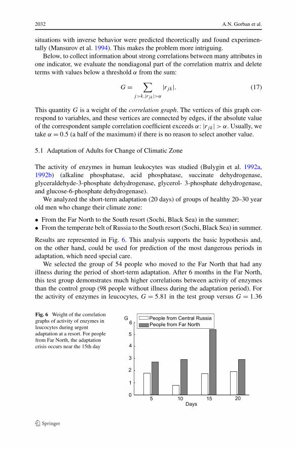
5.1 Adaptation of Adults for Change of Climatic Zone
The activity of enzymes in human leukocytes was studied (Bulygin et al. 1992a,1992b) (alkaline phosphatase, acid phosphatase, succinate dehydrogenase,glyceraldehyde-3-phosphate dehydrogenase, glycerol- 3-phosphate dehydrogenase,and glucose-6-phosphate dehydrogenase).
We analyzed the short-term adaptation (20 days) of groups of healthy 20–30 yearold men who change their climate zone:
• From the Far North to the South resort (Sochi, Black Sea) in the summer;• From the temperate belt of Russia to the South resort (Sochi, Black Sea) in summer.
Results are represented in Fig. 6. This analysis supports the basic hypothesis and,on the other hand, could be used for prediction of the most dangerous periods inadaptation, which need special care.
We selected the group of 54 people who moved to the Far North that had anyillness during the period of short-term adaptation. After 6 months in the Far North,this test group demonstrates much higher correlations between activity of enzymesthan the control group (98 people without illness during the adaptation period). Forthe activity of enzymes in leucocytes, G = 5.81 in the test group versus G = 1.36
Fig. 6 Weight of the correlationgraphs of activity of enzymes inleucocytes during urgentadaptation at a resort. For peoplefrom Far North, the adaptationcrisis occurs near the 15th day

Law of the Minimum Paradoxes 2033
in the control group. To compare the dimensionless variance for these groups, wenormalize the activity of enzymes to unite sample means (it is senseless to use thetrace of the covariance matrix without normalization because normal activities ofenzymes differ in order of magnitude). For the test group, the sum of the enzymevariances is 1.204, and for the control group it is 0.388.
5.2 Collapse of Correlations “on the Other Side of Crisis”: Acute HemolyticAnemia in Mice
It is very important to understand where the system is going: (i) to the bottom of thecrisis with possibility to recover after that bottom, (ii) to the normal state, from thebottom, or (iii) to the “no return” point, after which it cannot recover.
This problem was studied in many situations with analysis of fatal outcomes in on-cological (Mansurov et al. 1995) and cardiological (Strygina et al. 2000) clinics, andalso in special experiments with acute hemolytic anemia caused by phenylhydrazinein mice (Ponomarenko and Smirnova 1998). The main result here is: when approach-ing the no-return point, correlations destroy (G decreases), and variance typicallydoes continue to increase.
There exist no formal criterion to recognize the situation “on the other side ofcrisis.” Nevertheless, it is necessary to select situations for testing our hypothesis.Here, the “general practitioner point of view” (Goldstone 1952) can be of help. Fromsuch a point of view based on practical experience, the situation described below ison the other side of crisis: the acute hemolytic anemia caused by phenylhydrazine inmice with lethal outcome.
This effect was demonstrated in special experiments (Ponomarenko and Smirnova1998). Acute hemolytic anemia caused by phenylhydrazine was studied in CBAxlacmice. Dynamics of correlation between hematocrit, reticulocytes, erythrocytes,and leukocytes in blood is presented in Fig. 7. After phenylhydrazine injections(60 mg/kg, twice a day, with interval 12 hours) during first 5–6 days the amountof red cells decreased (Fig. 7), but at the 7th and 8th days this amount increasedbecause of spleen activity. After 8 days, most of the mice died. Weight of the correla-tion graph increase preceded the active adaptation response, but G decreased to zerobefore death (Fig. 7), while amount of red cells increased also at the last day.
5.3 Grassy Plants Under Trampling Load
The effect exists for plants, also. The grassy plants in oak tree-plants are studied(Karmanova et al. 1996). For analysis, the fragments of forests are selected, where the
Fig. 7 Adaptation anddisadaptation dynamics for miceafter phenylhydrazine injection
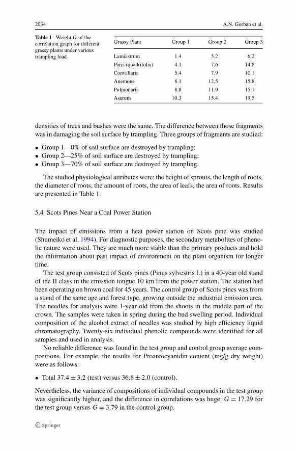
2034 A.N. Gorban et al.
Table 1 Weight G of thecorrelation graph for differentgrassy plants under varioustrampling load
Grassy Plant Group 1 Group 2 Group 3
Lamiastrum 1.4 5.2 6.2
Paris (quadrifolia) 4.1 7.6 14.8
Convallaria 5.4 7.9 10.1
Anemone 8.1 12.5 15.8
Pulmonaria 8.8 11.9 15.1
Asarum 10.3 15.4 19.5
densities of trees and bushes were the same. The difference between those fragmentswas in damaging the soil surface by trampling. Three groups of fragments are studied:
• Group 1—0% of soil surface are destroyed by trampling;• Group 2—25% of soil surface are destroyed by trampling;• Group 3—70% of soil surface are destroyed by trampling.
The studied physiological attributes were: the height of sprouts, the length of roots,the diameter of roots, the amount of roots, the area of leafs, the area of roots. Resultsare presented in Table 1.
5.4 Scots Pines Near a Coal Power Station
The impact of emissions from a heat power station on Scots pine was studied(Shumeiko et al. 1994). For diagnostic purposes, the secondary metabolites of pheno-lic nature were used. They are much more stable than the primary products and holdthe information about past impact of environment on the plant organism for longertime.
The test group consisted of Scots pines (Pinus sylvestris L) in a 40-year old standof the II class in the emission tongue 10 km from the power station. The station hadbeen operating on brown coal for 45 years. The control group of Scots pines was froma stand of the same age and forest type, growing outside the industrial emission area.The needles for analysis were 1-year old from the shoots in the middle part of thecrown. The samples were taken in spring during the bud swelling period. Individualcomposition of the alcohol extract of needles was studied by high efficiency liquidchromatography. Twenty-six individual phenolic compounds were identified for allsamples and used in analysis.
No reliable difference was found in the test group and control group average com-positions. For example, the results for Proantocyanidin content (mg/g dry weight)were as follows:
• Total 37.4 ± 3.2 (test) versus 36.8 ± 2.0 (control).
Nevertheless, the variance of compositions of individual compounds in the test groupwas significantly higher, and the difference in correlations was huge: G = 17.29 forthe test group versus G = 3.79 in the control group.

Law of the Minimum Paradoxes 2035
5.5 Choice of Coordinates and the Problem of Invariance
All indicators of the level of correlations are noninvariant with respect to transforma-tions of coordinates. For example, rotation to the principal axis annuls all the correla-tions. Dynamics of variance also depends on nonlinear transformations of scales. Di-mensionless variance of logarithms (or “relative variance”) often demonstrates morestable behavior especially when changes of mean values are large. The observed ef-fect depends on the choice of attributes. Nevertheless, many researchers observed itwithout a special choice of coordinate system. What does it mean? We can propose ahypothesis: the effect may be so strong that it is almost improbable to select a coor-dinate system where it vanishes. For example, if one accepts the Selye model (7), (8)then observability of the effect means that for typical nonzero values of ψ in crisis
l2kψ
2 > var(εk) (18)
for more than one value of k, where var stands for variance of the noise component(this is sufficient for increase of the correlations). If
ψ2∑
k
l2k �
∑
k
var(εk)
and the set of allowable transformations of coordinates is bounded (together withthe set of inverse transformations), then the probability to select randomly a coordi-nate system which violates condition (18) is small (for reasonable definitions of thisprobability and of the relation �).
6 Comparison to Econometrics
The simplest Selye’s model (7) seems very similar to the classical one-factor econo-metrics models (Campbell et al. 1997) which assume that the returns of stocks (ρi )are controlled by one factor, the “market” return M(t). In this model, for any stock
ρi(t) = ai + biM(t) + εi(t) (19)
where ρi(t) is the return of the ith stock at time t , ai and bi are real parameters, andεi(t) is a zero mean noise. In our models, the pressure of factor characterizes the timewindow and is slower variable than the return.
The main difference between models (7) and (19) could be found in the nonlinearcoupling (8) between the environmental property (the factor value f ) and the propertyof individuals (the resource amount R). Exactly this coupling causes separation ofa population into two groups: the well-adapted less correlated group and the highlycorrelated group with larger variances of individual properties and amount of resourcewhich is not sufficient for compensation of the factor load. Let us check whether sucha separation is valid for financial data.

2036 A.N. Gorban et al.
6.1 Data Description
For the analysis of correlations in financial systems, we used the daily closing val-ues for companies that are registered in the FTSE 100 index (Financial Times StockExchange Index). The FTSE 100 is a market-capitalization weighted index repre-senting the performance of the 100 largest UK-domiciled blue chip companies whichpass screening for size and liquidity. The index represents approximately 88.03% ofthe UK’s market capitalization. FTSE 100 constituents are all traded on the LondonStock Exchange’s SETS trading system. We selected 30 companies that had the high-est value of the capital (on the 1st of January 2007) and stand for different types ofbusiness as well. The list of the companies and business types is displayed in Table 2.
Data for these companies are available form the Yahoo!Finance web-site. For datacleaning, we use also information for the selected period available at the LondonStock Exchange web site. Let xi(t) denote the closing stock price for the ith com-pany at the moment t , where i = 1,30, t is the discrete time (the number of thetrading day). We analyze the correlations of logarithmic returns: xl
i (t) = ln xi (t)xi (t−1)
, insliding time windows of length p = 20, this corresponds approximately to 4 weeks of5 trading days. The correlation coefficients rij (t) for time moment t are calculated inthe time window [t −p, t −1], which strongly precedes t . Here, we calculate correla-tions between individuals (stocks), and for biological data we calculated correlationsbetween attributes. This corresponds to transposed data matrix.
6.2 Who Belongs to the Highly Correlated Group in Crisis
For analysis, we selected the time interval 10/04/2006–21/07/2006 that representsthe FTSE index decrease and restoration in spring and summer 2006 (more data areanalyzed in our e-print, Gorban et al. 2009). In Fig. 8, the correlation graphs arepresented for three time moments during the crisis development and three momentsof the restoration. The vertices of this graph correspond to stocks. These verticesare connected by solid lines is the correspondent correlation coefficient |rjk| ≥
√0.5
(√
0.5 = cos(π/4) ≈ 0.707), and by dashed lines if√
0.5 > |rjk| > 0.5.The correlation graphs from Fig. 8 show that in the development of this crisis
(10/04/2006–21/07/2006) the correlated group was formed mostly by two clusters:a financial cluster (banks and insurance companies) and an energy (oil/gas), mining,aerospace/defense, and travel cluster. At the bottom of the crisis, the correlated phaseincluded almost all stocks. The recovery followed a significantly different trajectory:the correlated phase in the recovery seems absolutely different from that phase in thecrisis development: There appeared the strong correlation between financial sectorand industry. This is a sign that after the crisis bottomed, the simplest Selye’s modelis not valid for a financial market. Perhaps, interaction between enterprises and redis-tribution of resources between them should be taken into account. We need additionalequations for dynamics of the available amounts of resource Ri for ith stock. Never-theless, appearance of the highly correlated phase in the development of the crisis inthe financial world followed the predictions of Selye’s model, at least, qualitatively.
Asymmetry between the drawups and the drawdowns of the financial market wasnoticed also in the analysis of the financial empirical correlation matrix of the 30companies which compose the Deutsche Aktienindex (DAX) (Drozdz et al. 2000).

Law of the Minimum Paradoxes 2037
Table 2 Thirty largest companies for analysis from the FTSE 100 index
Number Business type Company Abbreviation
1 Mining Anglo American plc AAL
2 BHP Billiton BHP
3 Energy (oil/gas) BG Group BG
4 BP BP
5 Royal Dutch Shell RDSB
6 Energy (distribution) Centrica CNA
7 National Grid NG
8 Finance (bank) Barclays plc BARC
9 HBOS HBOS
10 HSBC HLDG HSBC
11 Lloyds LLOY
12 Finance (insurance) Admiral ADM
13 Aviva AV
14 LandSecurities LAND
15 Prudential PRU
16 Standard Chartered STAN
17 Food production Unilever ULVR
18 Consumer Diageo DGE
19 goods/food/drinks SABMiller SAB
20 TESCO TSCO
21 Tobacco British American Tobacco BATS
22 Imperial Tobacco IMT
23 Pharmaceuticals AstraZeneca AZN
24 (inc. research) GlaxoSmithKline GSK
25 Telecommunications BT Group BTA
26 Vodafone VOD
27 Travel/leisure Compass Group CPG
28 Media (broadcasting) British Sky Broadcasting BSY
29 Aerospace/ BAE System BA
30 defence Rolls-Royce RR
The market mode was studied by principal component analysis (Plerou et al.2002). During periods of high market volatility, values of the largest eigenvalue ofthe correlation matrix are large. This fact was commented as a strong collective be-

2038 A.N. Gorban et al.
Fig. 8 Correlation graphs for six positions of sliding time window on interval 10/04/2006–21/07/2006.(a) Dynamics of FTSE100 (dashed line) and of G (solid line) over the interval, vertical lines correspondto the points that were used for the correlation graphs. (b) Thirty companies for analysis and their distri-butions over various sectors of economics. (c) The correlation graphs for the first three points, FTSE100decreases, the correlation graph becomes more connective. (d) The correlation graphs for the last threepoints, FTSE100 increases, the correlation graph becomes less connective
havior in regimes of high volatility. For this largest eigenvalue, the distribution ofcoordinates of the correspondent eigenvector has very remarkable properties:
• It is much more uniform than the prediction of the random matrix theory (Plerouet al. 2002 described this vector as “approximately uniform,” suggesting that allstocks participate in this “market mode”).
• Almost all components of that eigenvector have the same sign.• A large degree of cross correlations between stocks can be attributed to the influ-
ence of the largest eigenvalue and its corresponding eigenvector.
Two interpretations of this eigenvector were proposed (Plerou et al. 2002): It cor-responds either to the common strong factor that affects all stocks, or it represents

Law of the Minimum Paradoxes 2039
the “collective response” of the entire market to stimuli. Our observation supportsthis conclusion at the bottom of the crisis. At the beginning of the crisis, the corre-lated group includes stocks which are sensitive to the factor load, and other stocksare tolerant and form the less correlated group with the smaller variance. FollowingSelye’s model, we can conclude that the effect is the result of nonlinear coupling ofthe environmental factor load and the individual adaptation response.
7 Functional Decomposition and Integration of Subsystems
In the simple factor–resource Selye models, the adaptation response has no struc-ture: the organism just distributes the adaptation resource to neutralization of variousharmful factors. It is possible to make this model more realistic by decomposition.The resource is assigned not directly “against factors” but is used for activation andintensification of some subsystems.
We need to define the hierarchical structure of the organism to link the behaviorin across multiple scales. In integrative and computational physiology, it is necessaryto go both bottom-up and top-down approaches. The bottom-up approach goes fromproteins to cells, tissues, organs and organ systems, and finally to a whole organism(Crampin et al. 2004).
The top-down approach starts from a bird’s eye view of the behavior of thesystem—from the top or the whole and aims to discover and characterize biologicalmechanisms closer to the bottom—that is, the parts and their interactions (Crampinet al. 2004).
There is a long history of discussion of functional structure of the organism, andmany approaches are developed: from the Anokhin theory of functional systems (Su-dakov 2004) to the inspired by the General Systems approach theory of “FormalBiological Systems” (Chauvet 1999).
The notion of functional systems represents a special type of integration of physio-logical functions. Individual organs and tissue elements are selectively combined intoself-regulating systems organizations to achieve the necessary adaptive results impor-tant for the whole organism. The self-organization process is ruled by the adaptationneeds.
For decomposition of the models of physiological systems, the concept of princi-pal dynamic modes was developed (Marmarelis 1997, 2004).
In this section, we demonstrate how to decompose the factor-resource models ofthe adaptation of the organism to subsystems.
In general, the analysis of interaction of factors is decomposed to interaction offactors and subsystems. Compensation of the harm from each factor Fi requires ac-tivity of various systems. For every system Sj , a variable, activation level Ij is de-fined. Level 0 corresponds to a fully disabled subsystem (and for most of essentiallyimportant subsystems it implies death). For each factor Fi and every subsystem Sj , a“standard level” of activity ςij is defined. Roughly speaking, this level of activationof the subsystem Sj is necessary for neutralization of the unit value of the pressure ofthe factor Fi . If ςij = 0, then the subsystem Sj is not involved in the neutralizationof the factor Fi .

2040 A.N. Gorban et al.
Instead of ψ = f − arf (see (8)), we have to use
ωi = fi − minj, ςij �=0
{Ij
ςij
}
,
and the compensated value of the factor pressure Fi is
ψi ={
ωi, if ωi > 0;0, else.
(20)
In this model, resources are assigned not to neutralization of factors but for ac-tivation of subsystems. The activation intensity of the subsystem Sj depends on theadaptation resource rj , assigned to this subsystem:
Ij = αj rj and ωi = fi − minj,ςij �=0
{αj
ςij
rj
}
. (21)
For any given organization of the system of factors, optimization of fitness to-gether with definitions (20) and (21) lead to a clearly stated optimization problem.For example, for Liebig’s system of factors, we have to find distributions of rj thatgive solution to a problem:
maxi
ψi → min for rj ≥ 0,∑
j
rj ≤ R. (22)
If this minimum of maxima is positive (min(maxi ψi) > 0), then the optimal distrib-ution of resources is unique. If min(maxi ψi) = 0, then there exists a polyhedron ofoptimal distributions given by the system of inequalities:
αj
ςij
rj ≥ fi, rj ≥ 0 for all i, j,∑
j
rj ≤ R.
For the study of integration in the experiment, we use principal component analy-sis and find parameters of which systems give significant inputs in the first principalcomponents. Under the stress, the configuration of the subsystems, which are signif-icantly involved in the first principal components, changes (Svetlichnaia et al. 1997).
We analyzed interaction of cardiovascular and respiratory subsystems under ex-ercise tolerance tests at various levels of load. Typically, we observe the followingdynamics of the first factor composition. With increase of the load, coordinates boththe correlations of the subsystems attributes with the first factor increase up to somemaximal load which depend on the age and the health in the group of patients. Af-ter this maximum of integration, if the load continues to increase, then the level ofintegration decreases (Svetlichnaia et al. 1997).
Generalization of Selye’s models by decomposition creates a rich and flexible sys-tem of models for adaptation of hierarchically organized systems. Principal compo-nent analysis (Jolliffe 2002) with its various nonlinear generalizations (Gorban et al.2008; Gorban and Zinovyev 2009) gives a system of tools for extracting the informa-tion about integration of subsystems from the empirical data.

Law of the Minimum Paradoxes 2041
8 Conclusion
Due to the Law of the Minimum paradoxes, if we observe the Law of the Minimumin artificial systems, then under natural conditions adaptation will equalize the load ofdifferent factors and we can expect a violation of the Law of the Minimum. Inversely,if an artificial systems demonstrate significant violation of the law of the minimum,then we can expect that under natural conditions adaptation will compensate thisviolation.
This effect follows from the factor–resource models of adaptation and the idea ofoptimality applied to these models. We do not need an explicit form of generalizedfitness (which may be difficult to find), but use only the general properties that followfrom the Law of the Minimum (or, oppositely from the assumption of synergy).
Another consequence of the factor–resource models is the prediction of the ap-pearance of strongly correlated groups of individuals under an increase of the load ofenvironmental factors. Higher correlations in those groups do not mean that individ-uals become more similar, because the variance in those groups is also higher. Thiseffect is observed for financial market also and seems to be very general in ensemblesof systems which are adapting to environmental factors load.
Decomposition of the factor–resource models for the hierarchy of subsystems al-lows us to discuss integration of the subsystems in adaptation. For the explorativeanalysis of this integration in empirical data, the principal component analysis is thefirst choice: for the high level of integration different subsystems join in the mainfactors.
The most important shortcoming of the factor–resource models is the lack of dy-namics. In the present form, it describes adaptation as a single action, the distributionof the adaptation resource. We avoid any kinetic modeling. Nevertheless, adaptationis a process in time. We have to create a system of dynamical models.
References
Aumont, O., Maier-Reimer, E., Blain, S., & Monfray, P. (2003). An ecosystem model of the globalocean including Fe, Si, P colimitations. Glob. Biogeochem. Cycles, 17(2), 1060. doi:10.1029/2001GB001745.
Austin, M. (2007). Species distribution models and ecological theory: A critical assessment and somepossible new approaches. Ecol. Model., 200(1–2), 1–19.
Ballantyne, F. IV, Menge, D. N. L., Ostling, A., & Hosseini, P. (2008). Nutrient recycling affects autotrophand ecosystem stoichiometry. Am. Nat., 171(4), 511–523.
Bloom, A. J., Chapin, F. S. III, & Mooney, H. A. (1985). Resource limitation in plants—an economicanalogy. Annu. Rev. Ecol. Syst., 16, 363–392.
Bomze, I. M. (2002). Regularity vs. degeneracy in dynamics, games, and optimization: a unified approachto different aspects. SIAM Rev., 44, 394–414.
Breznitz, S. (Ed.) (1983). The denial of stress. New York: International Universities Press.Brown, G. C., & Cooper, C. E. (1993). Control analysis applied to a single enzymes: can an isolated
enzyme have a unique rate–limiting step? Biochem. J., 294, 87–94.Bulygin, G. V., Mansurov, A. S., Mansurova, T. P., & Smirnova, E. V. (1992a). Dynamics of parameters of
human metabolic system during the short-term adaptation. Institute of Biophysics, Russian Academyof Sciences, Preprint 180B, Krasnoyarsk.
Bulygin, G. V., Mansurov, A. S., Mansurova, T. P., Mashanov, A. A., & Smirnova, E. V. (1992b). Impactof health on the ecological stress dynamics. Institute of Biophysics, Russian Academy of Sciences,Preprint 185B, Krasnoyarsk.

2042 A.N. Gorban et al.
Cade, B. S., Terrell, J. W., & Schroeder, R. L. (1999). Estimating effects of limiting factors with regressionquantiles. Ecology, 80(1), 311–323.
Campbell, J. Y., Lo, A.-W., & MacKinlay, A. C. (1997). The econometrics of financial markets. Princeton:Princeton University Press.
Chapin, F. S. III, Schulze, E., & Mooney, H. A. (1990). The ecology and economics of storage in plants.Annu. Rev. Ecol. Syst., 21, 423–447.
Chauvet, G. A. (1999). S-propagators: a formalism for the hierarchical organization of physiological sys-tems. Application to the nervous and the respiratory systems. Int. J. Gen. Syst., 28(1), 53–96.
Chertov, O., Gorbushina, A., & Deventer, B. (2004). A model for microcolonial fungi growth on rocksurfaces. Ecol. Model., 177(3–4), 415–426.
Colborn, T., Dumanoski, D., & Meyers, J. P. (1996). Our stolen future: are we threatening our fertility,intelligence, and survival?—A scientific detective story. Dutton: Peguin Books.
Crampin, E. J., Halstead, M., Hunter, P., Nielsen, P., Noble, D., Smith, N., & Tawhai, M. (2004). Compu-tational physiology and the physiome project. Exp. Physiol., 89, 1–26.
Daly, H. E. (1991). Population and economics—a bioeconomic analysis. Popul. Environ., 12(3), 257–263.Danger, M., Daufresne, T., Lucas, F., Pissard, S., & Lacroix, G. (2008). Does Liebig’s law of the minimum
scale up from species to communities? Oikos, 117(11), 1741–1751.Droop, M. R. (1973). Some thoughts on nutrient limitation in algae. J. Phycol., 9, 264–272.Drozdz, S., Grümmer, F., Górski, A. Z., Ruf, F., & Speth, J. (2000). Dynamics of competition between
collectivity and noise in the stock market. Physica A, 287, 440–449.Egli, T., & Zinn, M. (2003). The concept of multiple-nutrient-limited growth of microorganisms and its
application in biotechnological processes. Biotechnol. Adv., 22(1–2), 35–43.Fisher, R. A. (1930). The genetical theory of natural selection. Oxford: Oxford University Press.Fusco, G., & Minelli, A. (2010). Phenotypic plasticity in development and evolution: facts and concepts.
Philos. Trans. R. Soc. B, 365(1540), 547–556.Gause, G. F. (1934). The struggle for existence. Baltimore: Williams and Wilkins. Online: http://www.
ggause.com/Contgau.htm.Goldstone, B. (1952). The general practitioner and the general adaptation syndrome. S. Afr. Med. J., 26,
88–92, 106–109. PMID: 14901129, 14913266.Gorban, A. N. (1984). Equilibrium encircling. Equations of chemical kinetics and their thermodynamic
analysis. Novosibirsk: Nauka.Gorban, A. N. (2004). Singularities of transition processes in dynamical systems: qualitative theory of
critical delays. Electron. J. Diff. Eqns. Monograph (Vol. 05). E-print: arXiv:chao-dyn/9703010.Gorban, A. N. (2007). Selection theorem for systems with inheritance. Math. Model. Nat. Phenom., 2(4),
1–45. E-print: arXiv:cond-mat/0405451 [cond-mat.stat-mech].Gorban, A. N., & Radulescu, O. (2008). Dynamic and static limitation in multiscale reaction networks,
revisited. Adv. Chem. Eng., 34, 103–173.Gorban, A. N., & Zinovyev, A. Y. (2009). Principal graphs and manifolds. In E. S. Olivas et al. (Eds.),
Handbook of research on machine learning applications and trends: algorithms, methods, and tech-niques (pp. 28–59). Hershey: IGI Global. E-print: arXiv:0809.0490 [cs.LG].
Gorban, A. N., Manchuk, V. T., & Petushkova (Smirnova), E. V. (1987). Dynamics of physiological para-methers correlations and the ecological-evolutionary principle of polyfactoriality. In Problemy Eko-logicheskogo Monitoringa i Modelirovaniya Ekosistem [The Problems of Ecological Monitoring andEcosystem Modelling] (pp. 187–198). Leningrad: Gidrometeoizdat.
Gorban, A. N., Kegl, B., Wunsch, D., & Zinovyev, A. (2008). Principal manifolds for data visualisationand dimension reduction. Lecture notes in computational science and engineering (Vol. 58). Berlin–Heidelberg–New York: Springer.
Gorban, A. N., Smirnova, E. V., & Tyukina, T. A. (2009). Correlations, risk and crisis: from physiology tofinance. E-print: arXiv:0905.0129 [physics.bio-ph].
Gorban, A. N., Radulescu, O., & Zinovyev, A. Y. (2010). Asymptotology of chemical reaction networks.Chem. Eng. Sci., 65, 2310–2324.
Greene, E. (1999). Phenotypic variation in larval development and evolution: polymorphism, polyphenism,and developmental reaction norms. In M. Wake & B. Hall (Eds.), The origin and evolution of larvalforms (pp. 379–410). San Diego: Academic Press.
Haldane, J. B. S. (1932). The causes of evolution. London: Longmans Green.Hennessy, D. A. (2009). Crop yield skewness under law of the minimum technology. Am. J. Agric. Econ.,
91(1), 197–208.Hoffman, R. J. (1978). Environmental uncertainty and evolution of physiological adaptation in colias but-
terflies. Am. Nat., 112(988), 999–1015.
Law of the Minimum Paradoxes 2043
Hutchinson, G. E. (1961). The paradox of the plankton. Am. Nat., 95, 137–145.Jolliffe, I. T. (2002). Principal component analysis, series. Springer series in statistics (Vol. 2). New York:
Springer.Karmanova, I. V., Razzhevaikin, V. N., & Shpitonkov, M. I. (1996). Application of correlation adaptometry
for estimating a response of herbaceous species to stress loadings. Dokl. Botanic. Sci., 346–348, 4–7.Translated from Dokl. Akad. Nauk SSSR, 346, 1996.
Kingsolver, J. G., & Pfennig, D. W. (2007). Patterns and power of phenotypic selection in nature. Bio-Science, 57(7), 561–572.
Kleene, S. C. (1956). Representation of events in nerve sets and finite automata. In J. McCarthy & C. Shan-non (Eds.), Automata studies (pp. 3–40). Princeton: Princeton University Press.
Kobe, R. K. (1996). Intraspecific variation in sapling mortality and growth predicts geographic variationin forest composition. Ecol. Monogr., 66(2), 181–201.
Kolokoltsov, V., & Maslov, V. (1997). Idempotent analysis and applications. Dordrecht: Kluwer Acad-emic.
Legovic, T., & Cruzado, A. (1997). A model of phytoplankton growth on multiple nutrients based on theMichaelis–Menten–Monod uptake, Droop’s growth and Liebig’s law. Ecol. Model., 99(1), 19–31.
Lerner, H. R. (Ed.) (1999). Plant responses to environmental stresses: from phytohormones to genomereorganization. New York: Dekker.
Litvinov, G. L. (2007). The Maslov dequantization idempotent and tropical mathematics: a brief introduc-tion. J. Math. Sci., 140(3), 426–444. arXiv:math/0507014 [math.GM].
Litvinov, G. L., & Maslov, V. P. (Eds.) (2005). Idempotent mathematics and mathematical physics. Con-temporary mathematics (Vol. 377). Providence: AMS.
Mansurov, A. S., Mansurova, T. P., Smirnova, E. V., Mikitin, L. S., & Pershin, A. V. (1994). How docorrelations between physiological parameters depend on the influence of different systems of stressfactors. In R. G. Khlebopros (Ed.), Global & regional ecological problems (pp. 499–516). Krasno-yarsk: Krasnoyarsk State Technical University Publ.
Mansurov, A. S., Mansurova, T. P., Smirnova, E. V., Mikitin, L. S., & Pershin, A. V. (1995). Human adapta-tion under influence of synergic system of factors (treatment of oncological patients after operation).Institute of Biophysics, Russian Academy of Sciences, Preprint 212B, Krasnoyarsk.
Marmarelis, V. Z. (1997). Modeling methodology for nonlinear physiological systems. Ann. Biomed. Eng.,25(2), 239–251.
Marmarelis, V. Z. (2004). Nonlinear dynamic modeling of physiological systems. New York: Wiley.Maynard-Smith, J. (1982). Evolution and the theory of games. Cambridge: Cambridge University Press.McCarty, R., & Pasak, K. (2000). Alarm phase and general adaptation syndrome. In G. Fink (Ed.), Ency-
clopedia of stress (Vol. 1, pp. 126–130). San Diego: Academic Press.McGill, B. (2005). A mechanistic model of a mutualism and its ecological and evolutionary dynamics.
Ecol. Model., 187(4), 413–425.Menge, D. N. L., & Weitz, J. S. (2009). Dangerous nutrients: Evolution of phytoplankton resource uptake
subject to virus attack. J. Theor. Biol., 257(1), 104–115.Metz, J. A. J., Nisbet, R. M., & Geritz, S. A. H. (1992). How should we define fitness for general ecological
scenarios. Trends Ecol. Evol., 7, 198–202.Milo, R., Hou, J. H., Springer, M., Brenner, M. P., & Kirschner, M. W. (2007). The relationship between
evolutionary and physiological variation in hemoglobin. PNAS USA, 104(43), 16998–17003.Nijland, G. O., Schouls, J., & Goudriaan, J. (2008). Integrating the production functions of Liebig
Michaelis-Menten, Mitscherlich and Liebscher into one system dynamics model. NJAS—WageningenJ. Life Sci., 55(2), 199–224.
Odum, E. P. (1971). Fundamentals of ecology (3rd ed.). Philadelphia–London–Toronto: Saunders.Oechssler, J., & Riedel, F. (2002). On the dynamic foundation of evolutionary stability in continuous
models. J. Econ. Theory, 107, 223–252.Ozden, M. Y. (2004). Law of the minimum in learning. Educ. Technol. Soc., 7(3), 5–8.Paris, Q. (1992). The return of von Liebig’s “Law of the Minimum”. Agron. J., 84, 1040–1046.Plerou, V., Gopikrishnan, P., Rosenow, B., Amaral, L. A. N., Guhr, T., & Stanley, H. E. (2002). Random
matrix approach to cross correlations in financial data. Phys. Rev. E, 65, 066126.Ponomarenko, L. D., & Smirnova, E. V. (1998). Dynamical characteristics of blood system in mice with
phenilhydrazin anemiya. In Proceeding of 9th international symposium “Reconstruction of home-ostasis” (Vol. 1, pp. 42–45), March 15–20, Krasnoyarsk, Russia.
Rockafellar, R. T. (1997). Convex analysis. Princeton: Princeton University Press.Saito, M. A., & Goepfert, T. J. (2008). Some thoughts on the concept of colimitation: Three definitions
and the importance of bioavailability. Limnol. Oceanogr., 53(1), 276–290.
2044 A.N. Gorban et al.
Salisbury, F. (1992). Plant physiology (4th ed.). Belmont: Wadsworth.Schkade, J. K., & Schultz, S. (2003). Occupational adaptation in perspectives. In P. Kramer, J. Hinojosa
& C. B. Royeen (Eds.), Perspectives in human occupation participation in life (pp. 181–221). Balti-more: Lippincott Williams & Wilkins. Chap. 7.
Sedov, K. R., Gorban’, A. N., Petushkova (Smirnova), E. V., Manchuk, V. T., & Shalamova, E. N., (1988).Correlation adaptometry as a method of screening of the population. Vestn. Akad. Med. Nauk SSSR,10, 69–75. PMID: 3223045.
Selye, H. (1938a). Adaptation energy. Nature, 141(3577), 926.Selye, H. (1938b). Experimental evidence supporting the conception of “adaptation energy”. Am. J. Phys-
iol., 123, 758–765.Semevsky, F. N., & Semenov, S. M. (1982). Mathematical modeling of ecological processes. Leningrad:
Gidrometeoizdat.Shaw, R. G., Geyer, C. J., Wagenius, S., Hangelbroek, H. H., & Etterson, J. R. (2008). Unifying life-history
analyses for inference of fitness and population growth. Am. Nat., 172, E35–E47.Shoresh, N., Hegreness, M., & Kishony, R. (2008). Evolution exacerbates the paradox of the plankton.
PNAS USA, 105(34), 12365–12369.Shumeiko, P. G., Osipov, V. I., & Kofman, G. B. (1994). Early detection of industrial emission impact
on Scots Pine needles by composition of phenolic compounds. In R. G. Khlebopros (Ed.), Global ®ional ecological problems (pp. 536–543). Krasnoyarsk: Krasnoyarsk State Technical UniversityPubl.
Sih, A., & Gleeson, S. K. (1995). A limits-oriented approach to evolutionary ecology. Trends Ecol. Evol.,10(9), 378–382.
Strygina, S. O., Dement’ev, S. N., Uskov, V. M., & Chernyshova, G. I. (2000). Dynamics of the system ofcorrelations between physiological parameters in patients after myocardial infarction. In Mathematicscomputer, education. Proceedings of conference (Vol. 7, pp. 685–689), Moscow.
Sudakov, K. V. (2004). Functional systems theory: a new approach to the question of the integration ofphysiological processes in the body. Neurosci. Behav. Physiol., 34(5), 495–500.
Svetlichnaia, G. N., Smirnova, E. V., & Pokidysheva, L. I. (1997). Correlational adaptometry as a methodfor evaluating cardiovascular and respiratory interaction. Fiziol. Chelov., 23(3), 58–62. PMID:9264951.
Thomson, J. D., Weiblen, G., Thomson, B. A., Alfaro, S., & Legendre, P. (1996). Untangling multiplefactors in spatial distributions: lilies, gophers and rocks. Ecology, 77, 1698–1715.
Tilman, D. (1980). Resources: a graphical-mechanistic approach to competition and predation. Am. Nat.,116(3), 362–393.
Tilman, D. (1982). Resource competition and community structure. Princeton: Princeton University Press.van den Berg, H. A. (1998). Multiple nutrient limitation in unicellulars: reconstructing Liebig’s law. Math.
Biosci., 149(1), 1–22.van der Ploeg, R. R., Böhm, W., & Kirkham, M. B. (1999). On the origin of the theory of mineral nutrition
of plants and the law of the minimum. Soil Sci. Soc. Am. J., 63, 1055–1062.Waxman, D., & Welch, J. J. (2005). Fisher’s microscope and Haldane’s ellipse. Am. Nat., 166, 447–457.West-Eberhard, M. J. (2003). Developmental plasticity and evolution. Oxford: Oxford University Press.Wutzler, T., & Reichstein, M. (2008). Colimitation of decomposition by substrate and decomposers—
a comparison of model formulations. Biogeosci. Discuss., 5, 163–190.Zinn, M., Witholt, B., & Egli, T. (2004). Dual nutrient limited growth: models experimental observations,
and applications. J. Biotechnol., 113(1–3), 263–279.Zuckerkandl, E., & Villet, R. (1988). Concentration-affinity equivalence in gene regulation: convergence
of genetic and environmental effects. PNAS USA, 85, 4784–4788.

![arXiv:quant-ph/0009009v5 8 Apr 2001[ML66b], [Sol77], [Cha87], [Cal94], [Vit97] satisfies the following intuitive condition: CONSTRAINT 3.1 ONTHENOTIONOFARANDOMSEQUENCE ONTHECOMMUTATIVEALPHABETΣ](https://img.pdfslide.net/doc/110x75/5fe6d8ac747c1e21f663f04d/arxivquant-ph0009009v5-8-apr-2001-ml66b-sol77-cha87-cal94-vit97.jpg)


![MINIMUM 6 76.[45] HYUNDAI/KIA MINIMUM](https://img.pdfslide.net/doc/110x75/61689563d394e9041f70d5f4/minimum-6-7645-hyundaikia-minimum.jpg)


