Marcos López de Prado

Lawrence Berkeley National LaboratoryComputational Research Division

ADVANCES IN QUANTITATIVE META-STRATEGIES

Key Points

2

• Quantitative Meta-Strategies (QMS) are quantitative strategies designed to manage investment strategies.

• As a field, QMS is the mathematical study of the decisions made by the supervisor of a team of investment managers, regardless of whether their investment style is systematic or discretionary.

• Some advantages that QMS offer are:

– Algorithmized investment processes can be tested and improved before being applied to a business.

– They provide objective and consistent oversight, and help prevent repeated mistakes.

– They are scalable and speed up quality improvement by limiting managerial frictions and biases.

SECTION IThe Art & Science of Investing

Investing is Not an Art

4

• Popular view: Investing is an Art because…

– It does not follow fixed rules (…unlike Art!)

– Like a sport or game, excellence cannot be taught, but it can only be learned through practice.

• Reality: Sports, Games, Arts increasingly rely on Math.

Any game can be studied mathematically. For decades it was thought that the sheer number of combinations involved in Chess would mean that computers would never beat top players. In 1996, IBM’s Deep Blue settled that question.

Today, some of the most successful hedge funds are math-oriented.

Investing is Not an Academic Endeavor

5

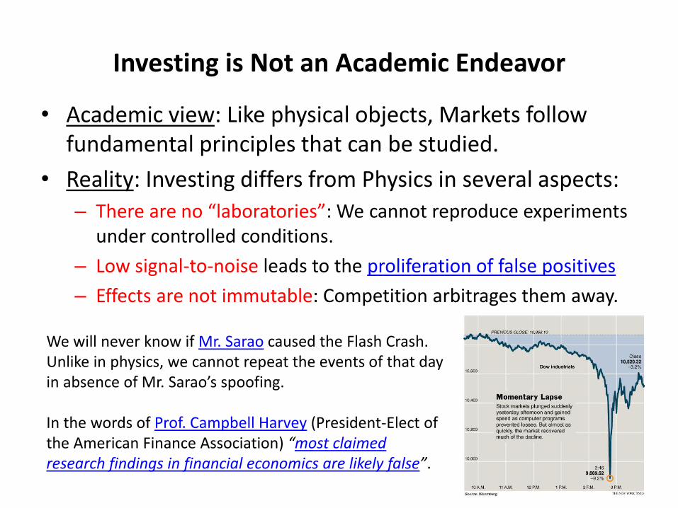
• Academic view: Like physical objects, Markets follow fundamental principles that can be studied.

• Reality: Investing differs from Physics in several aspects:

– There are no “laboratories”: We cannot reproduce experiments under controlled conditions.

– Low signal-to-noise leads to the proliferation of false positives

– Effects are not immutable: Competition arbitrages them away.

We will never know if Mr. Sarao caused the Flash Crash. Unlike in physics, we cannot repeat the events of that day in absence of Mr. Sarao’s spoofing.

In the words of Prof. Campbell Harvey (President-Elect of the American Finance Association) “most claimed research findings in financial economics are likely false”.

Investing is an Industrial Science

6

• In contrast with Academic Finance:

– Financial firms can conduct research in terms analogous to Scientific laboratories. E.g., deploy an execution algorithm and experiment with alternative configurations (market interaction).

– Financial firms can control for the increased probability of false positives that results from multiple testing, because they can take into account the results from all trials.

– Financial firms do not necessarily report their discoveries, thus discovered effects are more likely to persist.

• Conclusion #1: Empirical Finance discoveries are more likely to occur in the Industry than in Academia.

• QMS are investment processes geared towards taking advantage of those industrial discoveries.

SECTION IIStrategy Selection / PM Hiring

Strategy Selection Under Multiple Testing

8

• PROPOSITION #1: Suppose N independent trials following a Normal distribution, with mean

𝐸 𝑆𝑅𝑛 = 0 and variance 𝑉 𝑆𝑅𝑛 . Then, the

expected maximum Sharpe Ratio is

𝐸 𝑚𝑎𝑥 𝑆𝑅𝑛

≈ 𝑉 𝑆𝑅𝑛 1 − 𝛾 𝑍−1 1 −1

𝑁+ 𝛾𝑍−1 1 −

1

𝑁𝑒−1

where 𝜸 is the Euler-Mascheroni constant (approx. 0.5772), Z is the CDF of the Standard Normal and e is Euler’s number.

Backtest Overfitting

9

0

1

2

3

4

5

6

7

0 100 200 300 400 500 600 700 800 900 1000

Exp

ect

ed

Max

imu

m S

har

pe

Rat

io

Number of Trials (N)

Variance=1 Variance=4

Expected Maximum Sharpe Ratio as the number of independent trials N

grows, for 𝐸 𝑆𝑅𝑛 = 0

and 𝑉 𝑆𝑅𝑛 ∈ 1,4 .

Searching for empirical findings regardless of their theoretical basis is likely to magnify the

problem, as V 𝑆𝑅𝑛will increase when unrestrained by theory.

This is a consequence of pure random behavior. We will observe better candidates even

if there is no investment skill associated with this strategy class (𝐸 𝑆𝑅𝑛 = 0).

E max 𝑆𝑅𝑛 ≈ V 𝑆𝑅𝑛 1 − 𝛾 Z−1 1 −1

𝑁+ 𝛾Z−1 1 −

1

𝑁𝑒−1

The Backtest Overfitting Simulation Tool

10

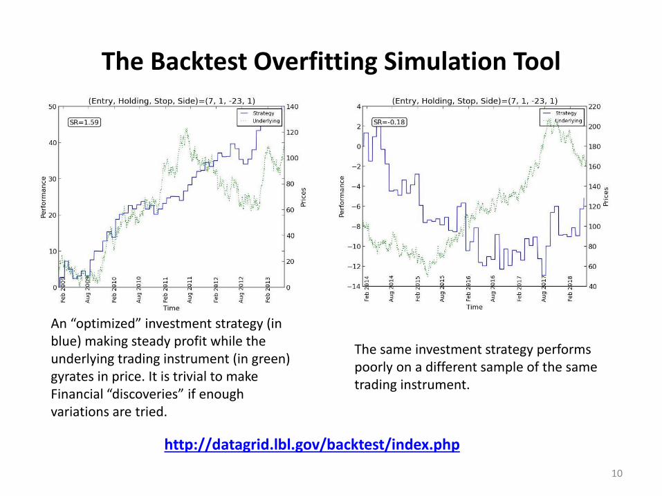
An “optimized” investment strategy (in blue) making steady profit while the underlying trading instrument (in green) gyrates in price. It is trivial to make Financial “discoveries” if enough variations are tried.

http://datagrid.lbl.gov/backtest/index.php

The same investment strategy performs poorly on a different sample of the same trading instrument.

The Deflated Sharpe Ratio (1/2)

11

• The Deflated Sharpe Ratio (DSR) corrects the inflationary effect of multiple trials, non-normal returns and shorter sample lengths:

𝐷𝑆𝑅 ≡ 𝑃𝑆𝑅 𝑆𝑅0 = 𝑍 𝑆𝑅 − 𝑆𝑅0 𝑇 − 1

1 − 𝛾3 𝑆𝑅 + 𝛾4 − 14

𝑆𝑅2

where

𝑆𝑅0 = 𝑉 𝑆𝑅𝑛 1 − 𝛾 𝑍−1 1 −1

𝑁+ 𝛾𝑍−1 1 −

1

𝑁𝑒−1

DSR is a Probabilistic Sharpe Ratio where the rejection threshold is adjusted to reflect the multiplicity of trials.

The Deflated Sharpe Ratio (2/2)

12

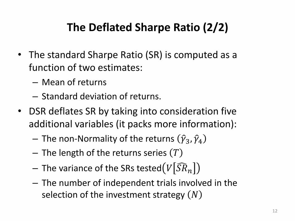
• The standard Sharpe Ratio (SR) is computed as a function of two estimates:

– Mean of returns

– Standard deviation of returns.

• DSR deflates SR by taking into consideration five additional variables (it packs more information):

– The non-Normality of the returns 𝛾3, 𝛾4– The length of the returns series 𝑇

– The variance of the SRs tested 𝑉 𝑆𝑅𝑛

– The number of independent trials involved in the selection of the investment strategy 𝑁

Numerical Example (1/2)

13

• An analyst uncovers a daily strategy with annualized SR=2.5,

after running N=100 independent trials, where 𝑉 𝑆𝑅𝑛 =1

2,

T=1250, 𝛾3 = −3 and 𝛾4 = 10.

• QUESTION: Is this a legitimate discovery, at a 95% conf.?

• ANSWER: No. There is only a 90% probability that the true Sharpe ratio is above zero.

– 𝑆𝑅0 =1

2∙2501 − 𝛾 𝑍−1 1 −

1

100+ 𝛾𝑍−1 1 −

1

100𝑒−1 ≈

0.1132

– 𝐷𝑆𝑅 ≈ 𝑍

2.5

250−0.1132 1249

1− −32.5

250+10−1

4

2.5

250

2= 0.9004.

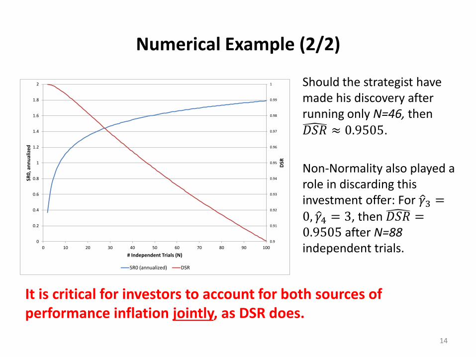
Numerical Example (2/2)

14

Should the strategist have made his discovery after running only N=46, then 𝐷𝑆𝑅 ≈ 0.9505.

Non-Normality also played a role in discarding this investment offer: For 𝛾3 =0, 𝛾4 = 3, then 𝐷𝑆𝑅 =0.9505 after N=88independent trials.

0.9

0.91

0.92

0.93

0.94

0.95

0.96

0.97

0.98

0.99

1

0

0.2

0.4

0.6

0.8

1

1.2

1.4

1.6

1.8

2

0 10 20 30 40 50 60 70 80 90 100

DSR

SR0

, an

nu

aliz

ed

# Independent Trials (N)

SR0 (annualized) DSR

It is critical for investors to account for both sources of performance inflation jointly, as DSR does.

SECTION IIIPortfolio Oversight

Finance and the Theory of Evolution

• Standard structural break tests (see Maddala and Kim [1999]) attempt to identify a “break” or permanent shiftfrom one regime to another within a time series.

• In contrast, the methodology we present here signals the emergence of a new regime as it happens, while it co-exists with the old regime (thus the mixture).

• This is a critical advantage, in terms of providing an early signal that a new investment style is emerging in a fund or portfolio.

• Conclusion #2: Evolutionary divergence attempts to signal the emergence of a new investment style before it is so prevalent that a “break” can be detected.

16

Action plan

1. Apply the EF3M algo for matching the track record’s moments (we have already seen this step).

2. Simulate path scenarios consistent with the matched moments.

3. Derive a distribution of scenarios based on that match.

4. Probability of Divergence (PD): Evaluate what percentile of the distribution corresponds with the PM’s recent performance.

Conclusion #3: PD assesses the evolutionary divergence by taking into account the entire distribution of the possible mixture parameters, based on the reliable moments.

17

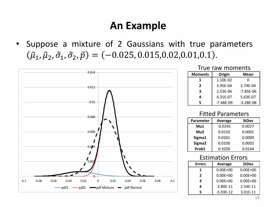
An Example

18

Errors Average StDev

1 0.00E+00 0.00E+00

2 0.00E+00 0.00E+00

3 0.00E+00 0.00E+00

4 -3.80E-11 2.54E-11

5 -5.93E-12 3.01E-11

Parameter Average StDev

Mu1 -0.0245 0.0027

Mu2 0.0150 0.0001

Sigma1 0.0201 0.0009

Sigma2 0.0100 0.0002

Prob1 0.1026 0.0144

0

0.002

0.004

0.006

0.008

0.01

0.012

0.014

-0.1 -0.08 -0.06 -0.04 -0.02 0 0.02 0.04 0.06 0.08 0.1

pdf1 pdf2 pdf Mixture pdf Normal

• Suppose a mixture of 2 Gaussians with true parameters 𝜇1, 𝜇2, 𝜎1, 𝜎2, 𝑝 = −0.025, 0.015,0.02,0.01,0.1 .

Moments Origin Mean

1 1.10E-02 0

2 3.95E-04 2.74E-04

3 2.53E-06 -7.85E-06

4 4.31E-07 5.63E-07

5 -7.48E-09 -3.28E-08

True raw moments

Fitted Parameters

Estimation Errors

Example 1 (1/2)

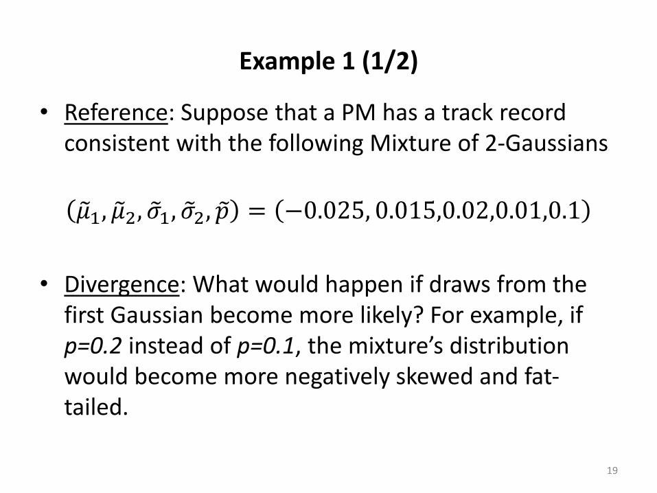
• Reference: Suppose that a PM has a track record consistent with the following Mixture of 2-Gaussians

𝜇1, 𝜇2, 𝜎1, 𝜎2, 𝑝 = −0.025, 0.015,0.02,0.01,0.1

• Divergence: What would happen if draws from the first Gaussian become more likely? For example, if p=0.2 instead of p=0.1, the mixture’s distribution would become more negatively skewed and fat-tailed.

19

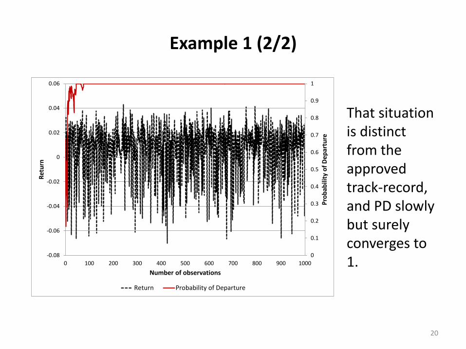
Example 1 (2/2)

That situation is distinct from the approved track-record, and PD slowly but surely converges to 1.

0

0.1

0.2

0.3

0.4

0.5

0.6

0.7

0.8

0.9

1

-0.08

-0.06

-0.04

-0.02

0

0.02

0.04

0.06

0 100 200 300 400 500 600 700 800 900 1000

Pro

bab

ility

of

De

par

ture

Ret

urn

Number of observations

Return Probability of Departure

20

Example 2 (1/2)

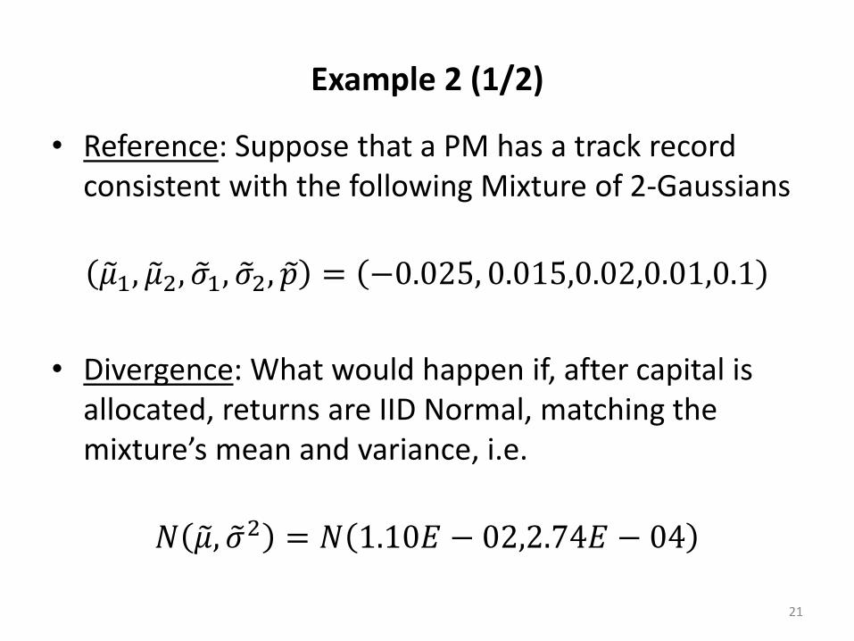
• Reference: Suppose that a PM has a track record consistent with the following Mixture of 2-Gaussians

𝜇1, 𝜇2, 𝜎1, 𝜎2, 𝑝 = −0.025, 0.015,0.02,0.01,0.1

• Divergence: What would happen if, after capital is allocated, returns are IID Normal, matching the mixture’s mean and variance, i.e.

𝑁 𝜇, 𝜎2 = 𝑁 1.10𝐸 − 02,2.74𝐸 − 04

21

Example 2 (2/2)

PD approaches 1, although the model cannot completely discard the possibility that these returns in fact were drawn from the reference mixture.

0

0.1

0.2

0.3

0.4

0.5

0.6

0.7

0.8

0.9

1

-0.06

-0.04

-0.02

0

0.02

0.04

0.06

0.08

0 100 200 300 400 500 600 700 800 900 1000

Pro

bab

ility

of

De

par

ture

Ret

urn

Number of observations

Return Probability of Departure

22

Example 3 (1/2)

• Reference: Suppose that a PM has a track record consistent with the following Mixture of 2-Gaussians

𝜇1, 𝜇2, 𝜎1, 𝜎2, 𝑝 = −0.025, 0.015,0.02,0.01,0.1

• Divergence: What would happen if, after capital is allocated, returns are IID Normal with a mean half the mixture’s and the same variance as the mixture…

𝑁 𝜇, 𝜎2 = 𝑁 5.5𝐸 − 03,2.74𝐸 − 04

23

Example 3 (2/2)

PD quickly converges to 1, as the model recognizes that those Normally distributed draws do not resemble the mixture’s simulated paths.

0

0.1

0.2

0.3

0.4

0.5

0.6

0.7

0.8

0.9

1

-0.06

-0.04

-0.02

0

0.02

0.04

0.06

0.08

0 100 200 300 400 500 600 700 800 900 1000

Pro

bab

ility

of

De

par

ture

Ret

urn

Number of observations

Return Probability of Departure

24

SECTION IVDecommissioning of Strategies / PMs

The Triple Penance Rule (1/2)

26

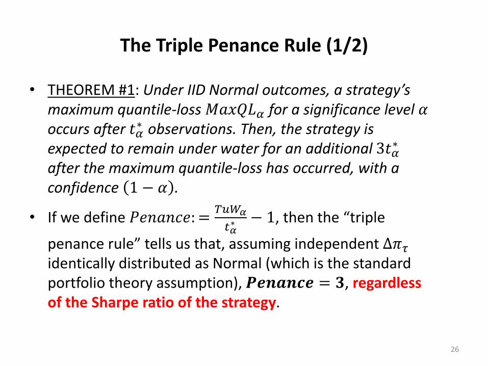
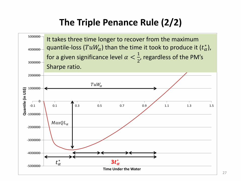
• THEOREM #1: Under IID Normal outcomes, a strategy’s maximum quantile-loss 𝑀𝑎𝑥𝑄𝐿𝛼 for a significance level 𝛼occurs after 𝑡𝛼

∗ observations. Then, the strategy is expected to remain under water for an additional 3𝑡𝛼

∗

after the maximum quantile-loss has occurred, with a confidence 1 − 𝛼 .

• If we define 𝑃𝑒𝑛𝑎𝑛𝑐𝑒: =𝑇𝑢𝑊𝛼

𝑡𝛼∗ − 1, then the “triple

penance rule” tells us that, assuming independent ∆𝜋𝜏identically distributed as Normal (which is the standard portfolio theory assumption), 𝑷𝒆𝒏𝒂𝒏𝒄𝒆 = 𝟑, regardless of the Sharpe ratio of the strategy.

The Triple Penance Rule (2/2)

27

-5000000

-4000000

-3000000

-2000000

-1000000

0

1000000

2000000

3000000

4000000

5000000

-0.1 0.1 0.3 0.5 0.7 0.9 1.1 1.3 1.5

Qu

anti

le (

in U

S$)

Time Under the Water

𝑀𝑎𝑥𝑄𝐿𝛼

𝑇𝑢𝑊𝛼

𝑡𝛼∗ 3𝒕𝜶

∗

It takes three time longer to recover from the maximum quantile-loss (𝑇𝑢𝑊𝛼) than the time it took to produce it (𝑡𝛼

∗ ),

for a given significance level 𝛼 <1

2, regardless of the PM’s

Sharpe ratio.

Example 1

28

-10000000

-5000000

0

5000000

10000000

15000000

20000000

0 0.5 1 1.5 2 2.5 3

Qu

an

tile

(in

US

$)

Time Under the Water

PM1 PM2

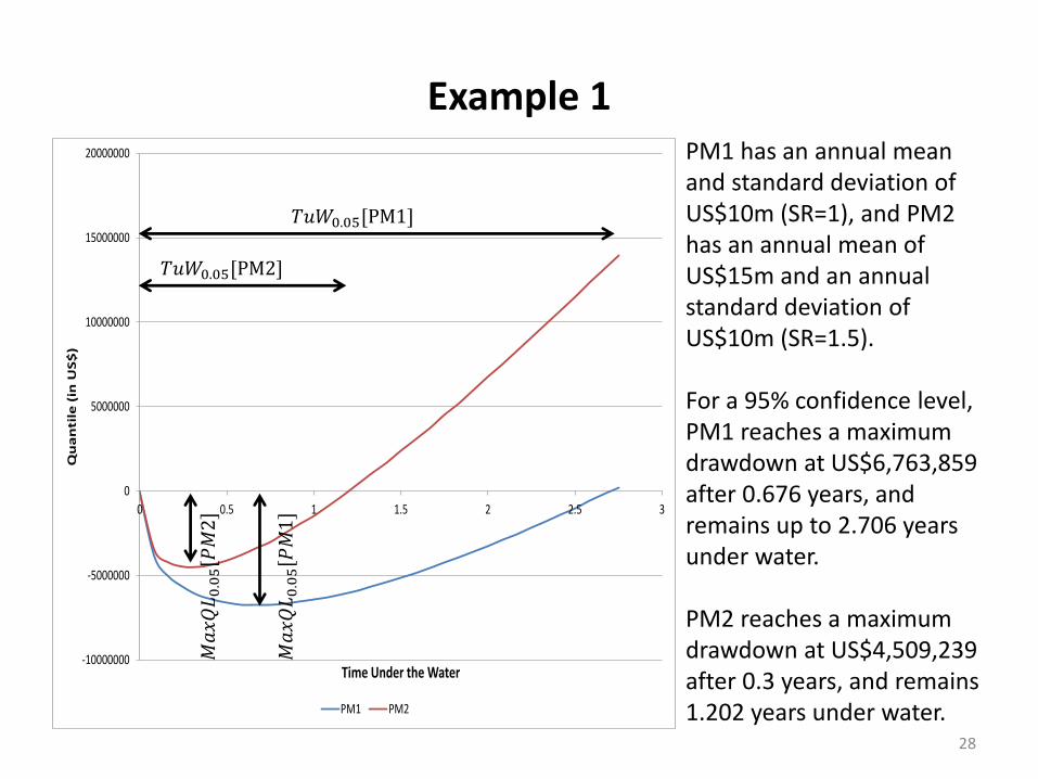
PM1 has an annual mean and standard deviation of US$10m (SR=1), and PM2 has an annual mean of US$15m and an annual standard deviation of US$10m (SR=1.5).

For a 95% confidence level, PM1 reaches a maximum drawdown at US$6,763,859 after 0.676 years, and remains up to 2.706 years under water.

PM2 reaches a maximum drawdown at US$4,509,239 after 0.3 years, and remains 1.202 years under water.

𝑇𝑢𝑊0.05[PM1]

𝑀𝑎𝑥𝑄𝐿0.05[𝑃𝑀1]

𝑇𝑢𝑊0.05[PM2]

𝑀𝑎𝑥𝑄𝐿0.05[𝑃𝑀2]

-8000000

-7000000

-6000000

-5000000

-4000000

-3000000

-2000000

-1000000

0

1000000

2000000

0 0.5 1 1.5 2 2.5

Qu

an

tile

(in

US

$)

Time Under the Water

PM1 PM2

Example 2

29

PM1 has an annual mean and standard deviation of US$10m (SR=1), and PM2 has an annual mean of US$15m and an annual standard deviation of US$10m (SR=1.5).

For a ~92% confidence level, PM1 reaches a maximum drawdown at US$5,000,000 after 0.5 years, and remains up to 2 years under water.

For a ~98% confidence level, PM2 reaches a maximum drawdown at US$7,500,000 after 0.5 years, and remains up to 2 years under water.

𝑇𝑢𝑊0.08 𝑃𝑀1 = 𝑇𝑢𝑊0.02 𝑃𝑀2

𝑀𝑎𝑥𝑄𝐿0.08[𝑃𝑀1]

𝑀𝑎𝑥𝑄𝐿0.02[𝑃𝑀2]

3𝒕𝜶∗𝑡𝛼

∗

A Better Way to Stop-Out

30

• Given a realized performance 𝜋𝑡 < 0 and assuming IID Normal returns with mean 𝜇 > 0, the Implied Time Under Water (ITuW) is

𝐼𝑇𝑢𝑊 𝜋𝑡 = 𝜋𝑡

2

𝜇2𝑡− 2

𝜋𝑡𝜇+ 𝑡

• The above equation translates a realized loss into time under water.

• It makes sense stopping-out strategies based on their expected recovery time, rather than waiting for a fixed loss threshold to be hit.

Implications of the Triple Penance Rule

31

1. It makes possible the translation of drawdowns in terms of time under water.

2. It sets expectations regarding how long it may take to earn performance fee (for a certain confidence level).– The remaining time under water may be so long that

withdrawals are expected. This has implications for the firm’s cash management.

3. It shows that the penance period is independent of the Sharpe ratio (in the IID Normal case).– E.g., if a PM makes a fresh new bottom after being one year

under water, it may take him 3 years to recover, under the confidence level associated with that loss. This holds true whether that PM has a Sharpe of 1 or a Sharpe of 10.

SECTION VConclusions

Pros & Cons of Classic Approaches vs. QMS

33

Practical

ApplicationClassic approach Quantitative Meta-Strategy

Hiring

(Example 1)

Interview candidates with SR (or any

other performance statistic) and track

record length above a given threshold.

Pros: Trivial to implement.

Cons: Unknown (possibly high)

probability of hiring unskilled PMs.

Design an interview process that recognizes the variables that

affect the probability of making the wrong hire:

False positive rate.

False negative rate.

Skill-to-unskilled odds ratio.

Number of independent trials.

Sampling mechanism.

Pros: It is objective and can be improved over time, based on

measurable outcomes.

Cons: More laborious.

Oversight

(Example 2)

Allocate capital as if PMs were asset

classes.

Pros: Trivial to implement.

Cons: Correlations are unstable,

meaningless. Risks are likely to be

concentrated.

Recognize that PMs styles evolve over time, as they adapt to

a changing environment.

Pros: It provides an early signal while the style is still

emerging. Allocations can be revised before it is too late.

Cons: Allocation revisions may be needed on an irregular

calendar frequency.

Stop-Out

(Example 3)

Stop-out a PM once a certain loss limit

has been exceeded.

Pros: Trivial to implement.

Cons: It allows preventable problems to

grow until it is too late.

For any drawdown, large or small, determine the expected

time underwater and monitor every recovery. Even if a loss is

small, a failure to recover within the expected timeframe

indicates a latent problem.

Pros: Proactive. Address problems before they force a stop-

out.

Cons: PMs may feel under tighter scrutiny.

THANKS FOR YOUR ATTENTION!

34

SECTION VIThe stuff nobody reads

Bibliography

• Bailey, D., J. Borwein, M. López de Prado and J. Zhu (2015): “The Probability of Backtest Overfitting.” Journal of Computational Finance, forthcoming. Available at: http://ssrn.com/abstract=2326253

• Bailey, D., J. Borwein, M. López de Prado and J. Zhu (2014): “Pseudo-Mathematics and Financial Charlatanism: The Effects of Backtest Overfitting on Out-Of-Sample Performance.” Notices of the American Mathematical Society, 61(5), May. Available at: http://ssrn.com/abstract=2308659

• Bailey, D. and M. López de Prado (2012): “The Sharpe Ratio Efficient Frontier.” Journal of Risk, 15(2), Winter. Available at http://ssrn.com/abstract=1821643

• Bailey, D. and M. López de Prado (2015): “Stop-Outs Under Serial Correlation and 'The Triple Penance Rule’”, Journal of Risk, forthcoming. Available at http://ssrn.com/abstract=2201302

• López de Prado, M. (2015): “Quantitative Meta-Strategies”, Practical Applications (IIJ), 2(3), Spring. Available at http://ssrn.com/abstract=2547325

• López de Prado, M. and M. Foreman (2013): A Mixture of Gaussians Approach to Mathematical Portfolio Oversight: The EF3M Algorithm”, Quantitative Finance, 14(5): 913-930. Available at http://ssrn.com/abstract=1931734

36

Bio

Marcos López de Prado is Senior Managing Director at Guggenheim Partners. He is also a ResearchFellow at Lawrence Berkeley National Laboratory's Computational Research Division (U.S. Departmentof Energy’s Office of Science), where he conducts unclassified research in the mathematics of large-scale financial problems and supercomputing.

Before that, Marcos was Head of Quantitative Trading & Research at Hess Energy Trading Company (thetrading arm of Hess Corporation, a Fortune 100 company) and Head of Global Quantitative Research atTudor Investment Corporation. In addition to his 17 years of trading and investment managementexperience at some of the largest corporations, he has received several academic appointments,including Postdoctoral Research Fellow of RCC-Harvard University and Visiting Scholar at CornellUniversity. Marcos earned a Ph.D. in Financial Economics (2003), a second Ph.D. in MathematicalFinance (2011) from Complutense University, is a recipient of the National Award for Excellence inAcademic Performance by the Government of Spain (National Valedictorian, 1998) among other awards,and was admitted into American Mensa with a perfect test score.

Marcos serves on the Editorial Board of the Journal of Portfolio Management (IIJ) and the Journal ofInvestment Strategies (Risk). He has collaborated with ~30 leading academics, resulting in some of themost read papers in Finance (SSRN), four international patent applications on High Frequency Trading,three textbooks, numerous publications in the top Mathematical Finance journals, etc. Marcos has anErdös #2 and an Einstein #4 according to the American Mathematical Society.

37

Disclaimer

• The views expressed in this document are the authors’ and do not necessarily reflect those of the organizations he is affiliated with.

• No investment decision or particular course of action is recommended by this presentation.

• All Rights Reserved.

38

Notice:

The research contained in this presentation is the result of a continuing collaboration with

David H. Bailey, Berkeley LabJon M. Borwein, FRSC, AAASMatthew Foreman, UC-Irvine

The full paper is available at:http://ssrn.com/abstract=2547325

For additional details, please visit:http://ssrn.com/author=434076

www.QuantResearch.info