Embed Size (px)
DESCRIPTION
Outline Description of tkGeometry tools tkLayout (operational) tkMaterial (operational) - validation tk2CMSSW (under development) Outlook Overview of (some) studies done so far Endcap with rectangular detectors Modelling of different options Outlook. - PowerPoint PPT Presentation
Citation preview
1
Layout studiesTools and results – general overview
OutlineDescription of tkGeometry tools• tkLayout (operational)• tkMaterial (operational)
- validation• tk2CMSSW (under development)• Outlook
Overview of (some) studies done so far• Endcap with rectangular detectors• Modelling of different options• Outlook
2
tkGeometry tools
tkLayout: generation of detector geometry • Starting from (relatively) small n of input parameters and assumptions• Basic geometrical validation (n of hits)• Calculation of overall basic parameters (surface, channels, power…)
tkMaterial: modelling of detector material• Simplified modelling with small n of input parameters• Creation of (additional) inactive volumes• Produce radpidity profile of radiation and interaction lengths
tkCMSSW: Creation of geometry files for CMSSW
• Should be readable by IGUANA• Tracking is another story…
3
tkLayout
Two configuration files
Geometry.cfg• Defines the geometry of active surfaces
Module_type.cfg• Defines which type of module populates each surface
(layer/ring/disk)
Some (non exhaustive) examples in the following slides
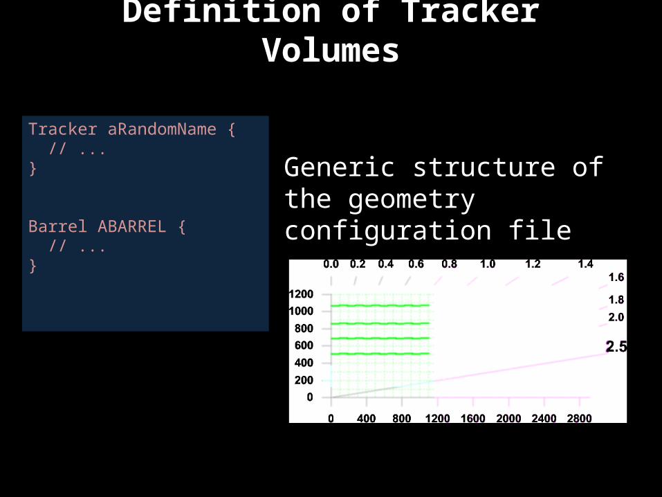
Definition of Tracker Volumes
Tracker aRandomName { // ...}
Barrel ABARREL { // ...}
Generic structure of the geometry configuration file
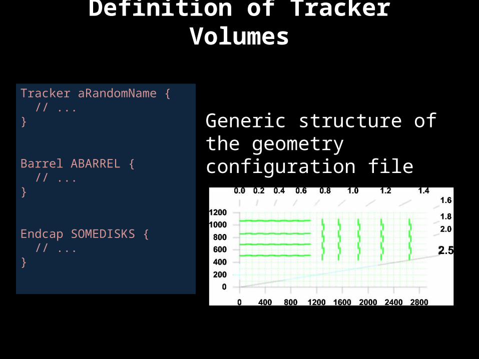
Definition of Tracker Volumes
Tracker aRandomName { // ...}
Barrel ABARREL { // ...}
Endcap SOMEDISKS { // ...}
Generic structure of the geometry configuration file
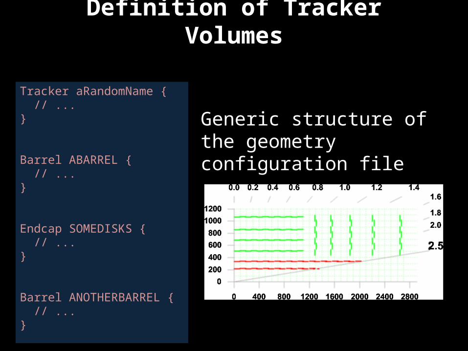
Definition of Tracker Volumes
Tracker aRandomName { // ...}
Barrel ABARREL { // ...}
Endcap SOMEDISKS { // ...}
Barrel ANOTHERBARREL { // ...}
Generic structure of the geometry configuration file
7
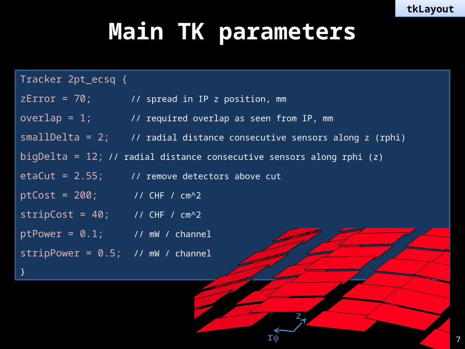
Main TK parameters
Tracker 2pt_ecsq {
zError = 70; // spread in IP z position, mm
overlap = 1; // required overlap as seen from IP, mm
smallDelta = 2; // radial distance consecutive sensors along z (rphi)
bigDelta = 12; // radial distance consecutive sensors along rphi (z)
etaCut = 2.55; // remove detectors above cut
ptCost = 200; // CHF / cm^2
stripCost = 40; // CHF / cm^2
ptPower = 0.1; // mW / channel
stripPower = 0.5; // mW / channel
}
tkLayout
rf
z
8
ModulestkLayout
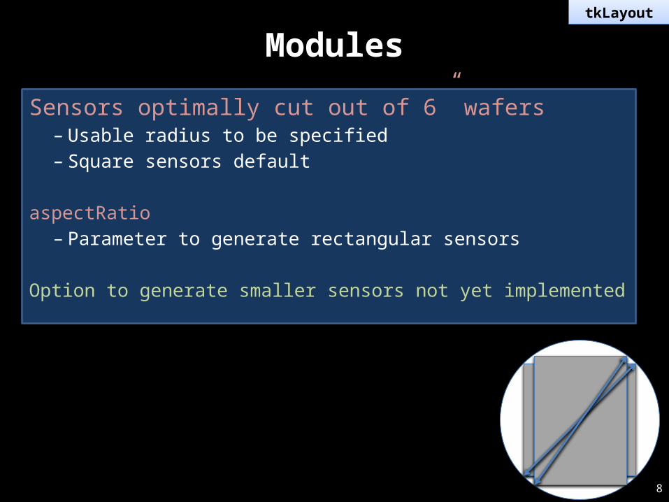
Sensors optimally cut out of 6” wafers– Usable radius to be specified– Square sensors default
aspectRatio– Parameter to generate rectangular sensors
Option to generate smaller sensors not yet implemented
9
Barrel geometry
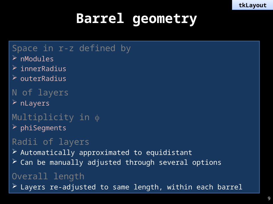
Space in r-z defined by nModules innerRadius outerRadius
N of layers nLayers
Multiplicity in f phiSegments
Radii of layers Automatically approximated to equidistant Can be manually adjusted through several options
Overall length Layers re-adjusted to same length, within each barrel
tkLayout
10
Barrel special options
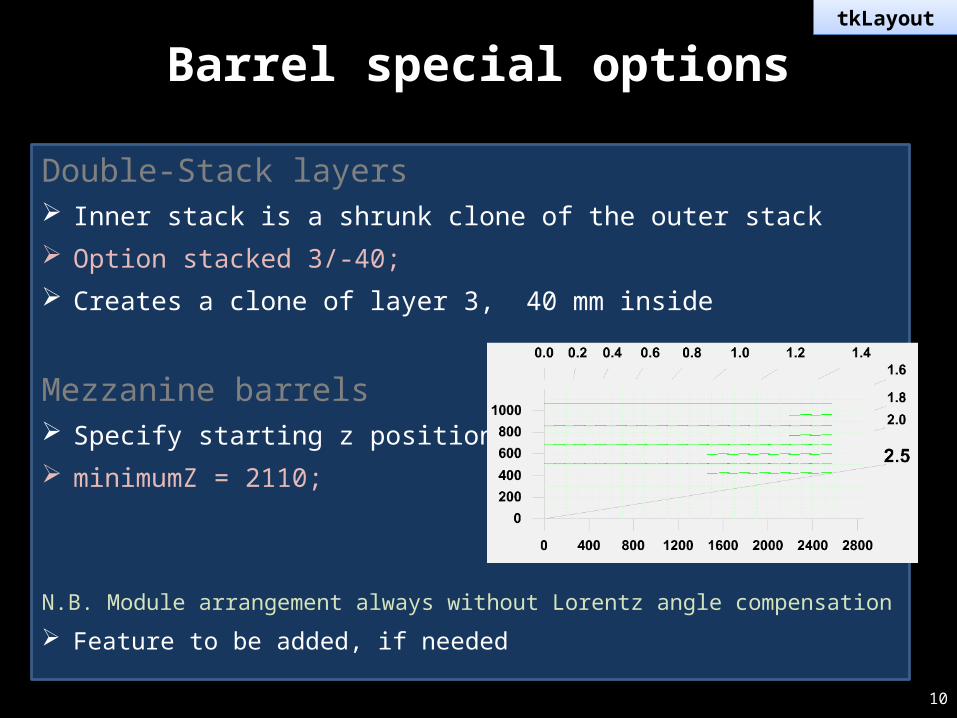
Double-Stack layers Inner stack is a shrunk clone of the outer stack Option stacked 3/-40;
Creates a clone of layer 3, 40 mm inside
Mezzanine barrels Specify starting z position minimumZ = 2110;
N.B. Module arrangement always without Lorentz angle compensation
Feature to be added, if needed
tkLayout
11
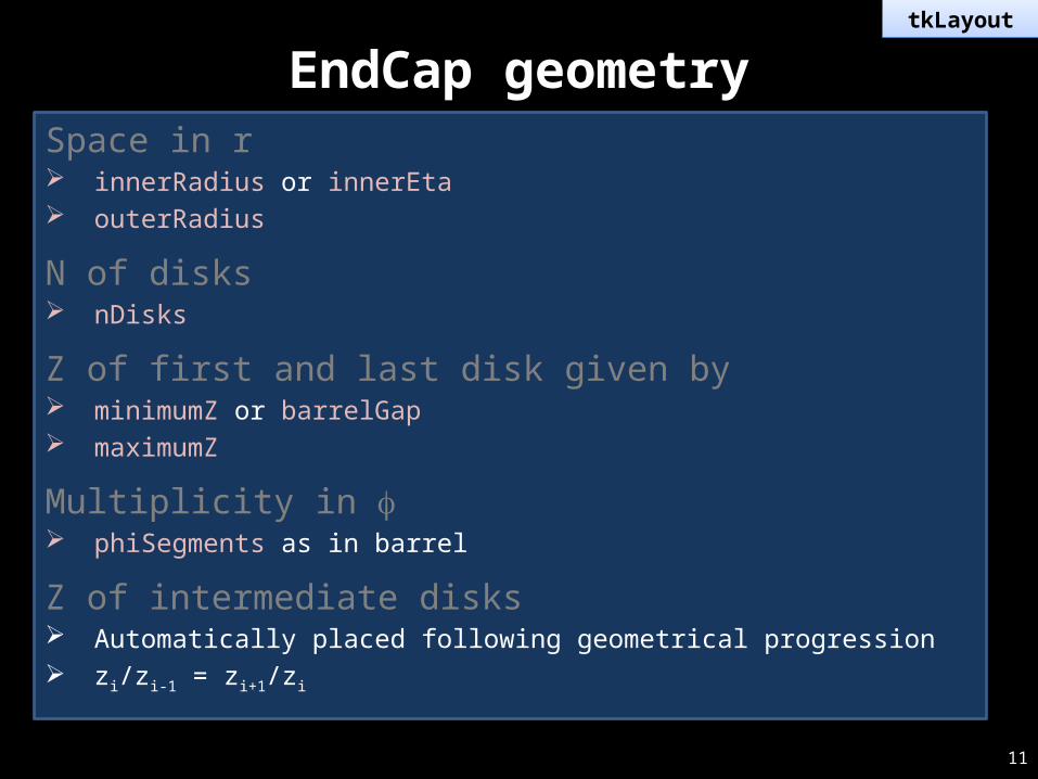
EndCap geometrySpace in r innerRadius or innerEta outerRadius
N of disks nDisks
Z of first and last disk given by minimumZ or barrelGap maximumZ
Multiplicity in f phiSegments as in barrel
Z of intermediate disks Automatically placed following geometrical progression zi/zi-1 = zi+1/zi
tkLayout
12
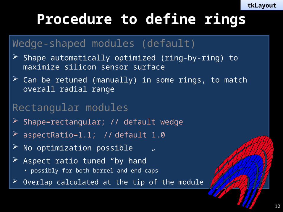
Procedure to define rings
Wedge-shaped modules (default) Shape automatically optimized (ring-by-ring) to maximize silicon sensor
surface
Can be retuned (manually) in some rings, to match overall radial range
Rectangular modules Shape=rectangular; // default wedge
aspectRatio=1.1; // default 1.0
No optimization possible
Aspect ratio tuned “by hand”• possibly for both barrel and end-caps
Overlap calculated at the tip of the module
tkLayout
13
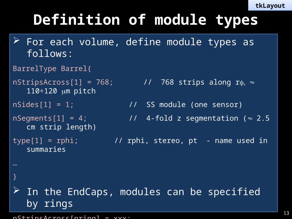
Definition of module types For each volume, define module types as follows:BarrelType Barrel{
nStripsAcross[1] = 768; // 768 strips along r , ≈ f 110÷120 mm pitch
nSides[1] = 1; // SS module (one sensor)
nSegments[1] = 4; // 4-fold z segmentation (≈ 2.5 cm strip length)
type[1] = rphi; // rphi, stereo, pt - name used in summaries
…
}
In the EndCaps, modules can be specified by ringsnStripsAcross[nring] = xxx;
Or by ring and disknStripsAcross[nring,ndisk] = xxx;
tkLayout
14
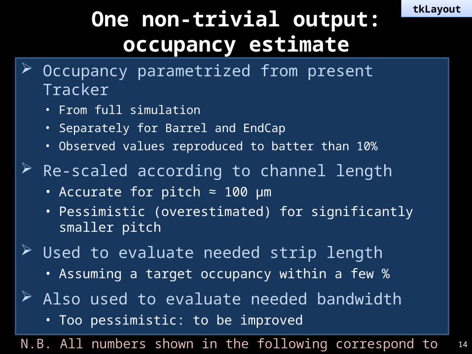
One non-trivial output: occupancy estimate
Occupancy parametrized from present Tracker• From full simulation• Separately for Barrel and EndCap• Observed values reproduced to batter than 10%
Re-scaled according to channel length• Accurate for pitch ≈ 100 μm• Pessimistic (overestimated) for significantly smaller pitch
Used to evaluate needed strip length• Assuming a target occupancy within a few %
Also used to evaluate needed bandwidth• Too pessimistic: to be improved
N.B. All numbers shown in the following correspond to 400 mb/BX!!
tkLayout
15
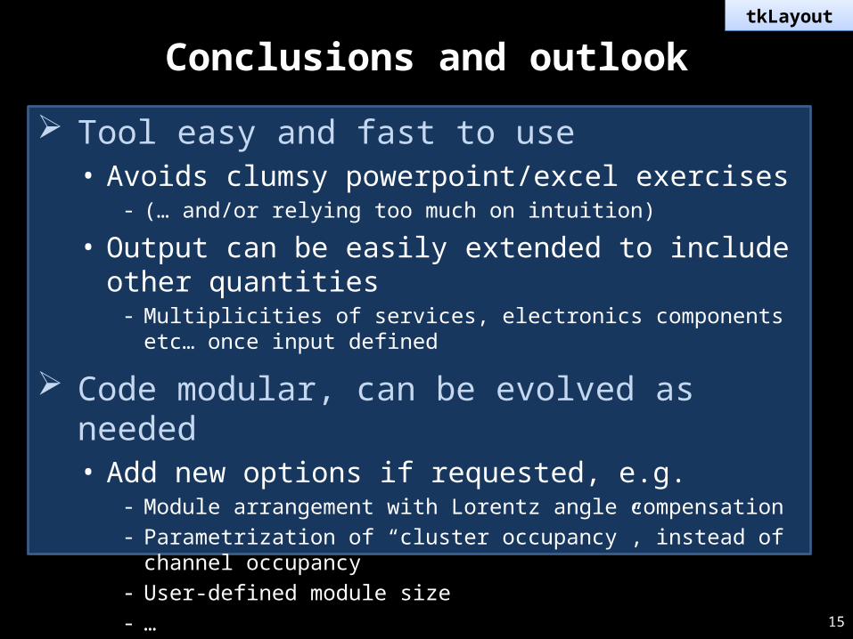
Conclusions and outlook
Tool easy and fast to use• Avoids clumsy powerpoint/excel exercises
- (… and/or relying too much on intuition)
• Output can be easily extended to include other quantities- Multiplicities of services, electronics components etc… once input defined
Code modular, can be evolved as needed• Add new options if requested, e.g.
- Module arrangement with Lorentz angle compensation- Parametrization of “cluster occupancy”, instead of channel occupancy- User-defined module size- …
tkLayout
16
tkMaterial
Creation of volumes• Starting from a geometry generated with tkLayout
Modelling of materials• Strategy chosen to limit complexity and maximize flexibility
Configuration file• Some examples
17
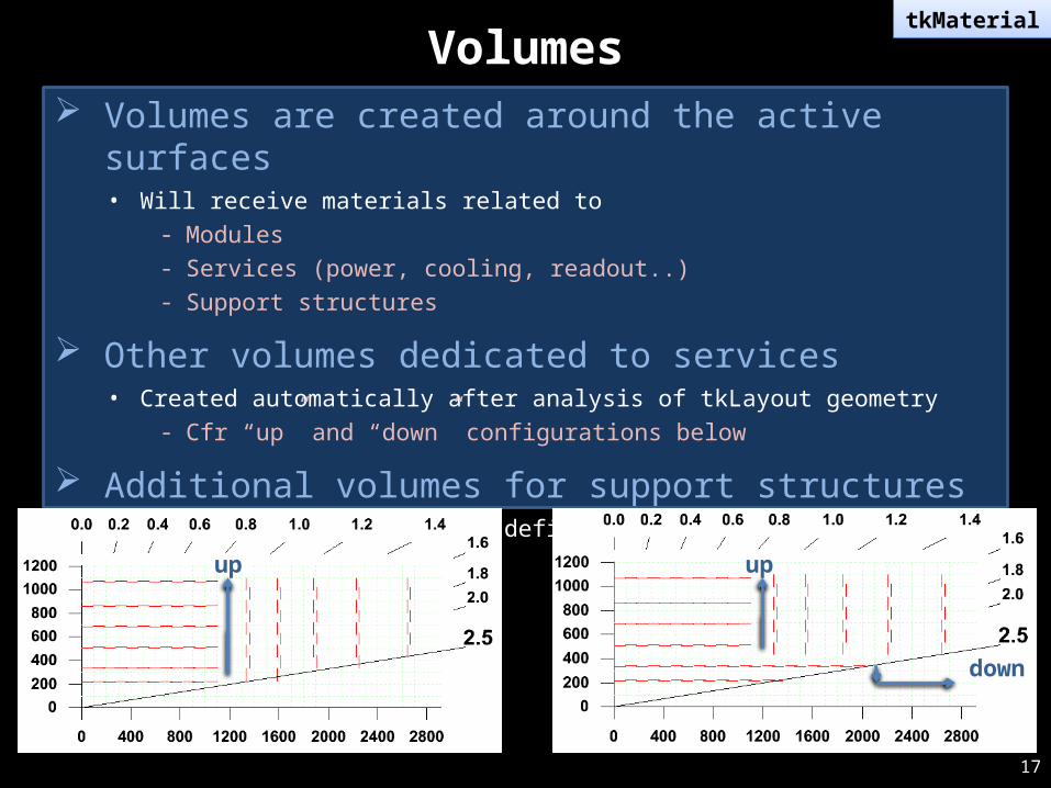
Volumes Volumes are created around the active surfaces
• Will receive materials related to- Modules- Services (power, cooling, readout..)- Support structures
Other volumes dedicated to services• Created automatically after analysis of tkLayout geometry
- Cfr “up” and “down” configurations below
Additional volumes for support structures• Some automatic, some user-defined
- …
tkMaterial
up up
down
18
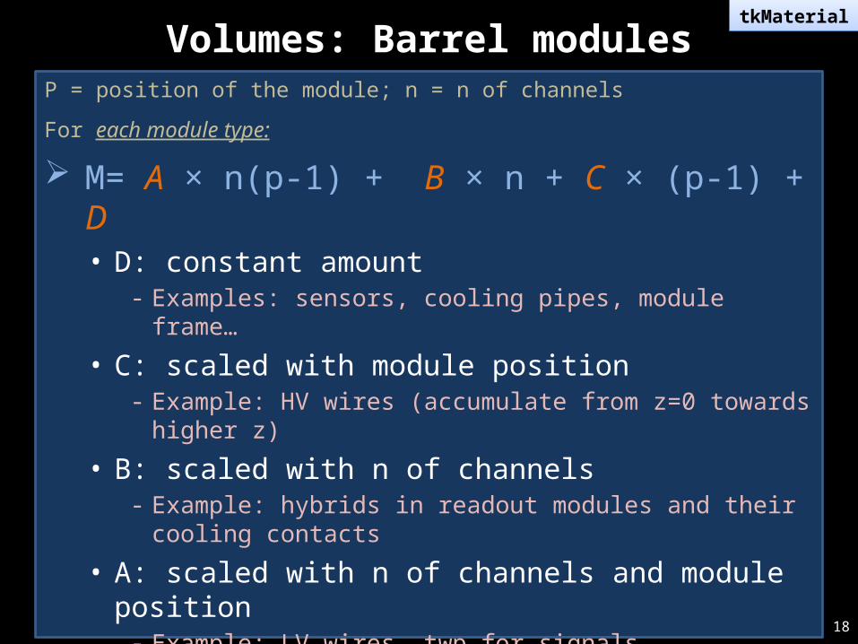
Volumes: Barrel modulesP = position of the module; n = n of channels
For each module type:
M= A × n(p-1) + B × n + C × (p-1) + D• D: constant amount
- Examples: sensors, cooling pipes, module frame…
• C: scaled with module position- Example: HV wires (accumulate from z=0 towards higher z)
• B: scaled with n of channels- Example: hybrids in readout modules and their cooling contacts
• A: scaled with n of channels and module position- Example: LV wires, twp for signals….
Flag assigned to each contribution• “L” = Local; “E” = exiting
- Contribution with “E” flag are taken as input for module services
tkMaterial
19
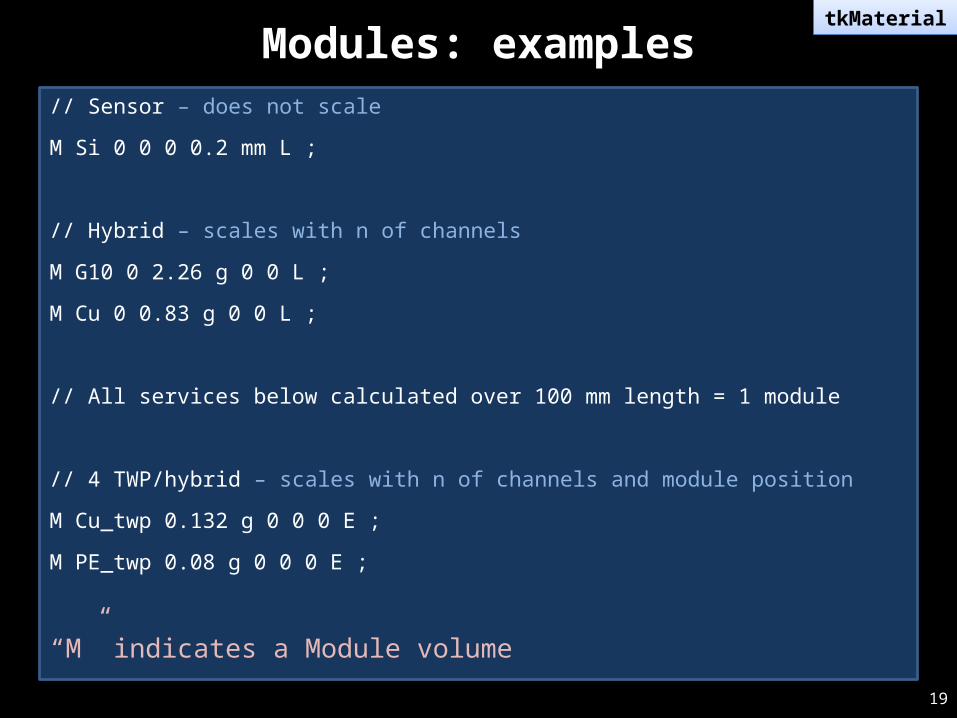
Modules: examples// Sensor – does not scale
M Si 0 0 0 0.2 mm L ;
// Hybrid – scales with n of channels
M G10 0 2.26 g 0 0 L ;
M Cu 0 0.83 g 0 0 L ;
// All services below calculated over 100 mm length = 1 module
// 4 TWP/hybrid – scales with n of channels and module position
M Cu_twp 0.132 g 0 0 0 E ;
M PE_twp 0.08 g 0 0 0 E ;
“M” indicates a Module volume
tkMaterial
20
Volumes: EndCap modules
Same concept as for barrel, but
Different rings in a disk may have different module flavours• While modules are all identical along a Barrel rod/string
Services from inner rings decrease in density while running outwards on a disk• Simple scaling with ring # does not work
Solution
Explicit calculation of material from inner rings• Taking into account module types and density scaling
tkMaterial
21
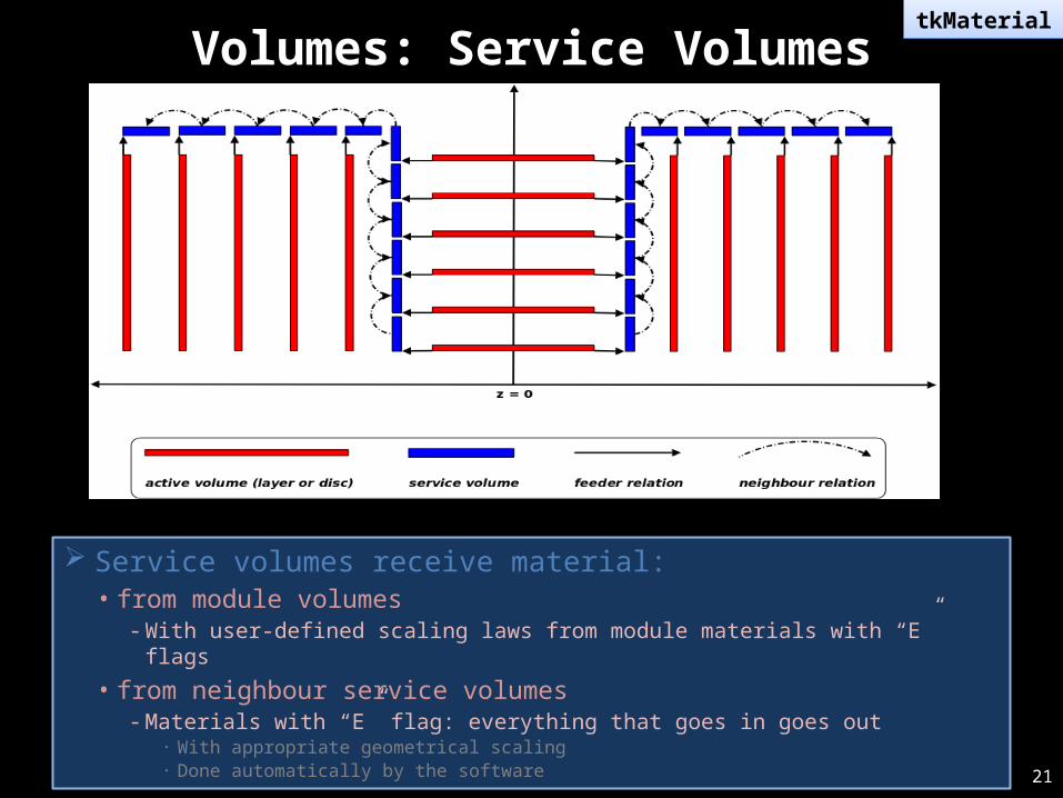
Volumes: Service VolumestkMaterial
Service volumes receive material:• from module volumes
- With user-defined scaling laws from module materials with “E” flags
• from neighbour service volumes- Materials with “E” flag: everything that goes in goes out
· With appropriate geometrical scaling· Done automatically by the software
22
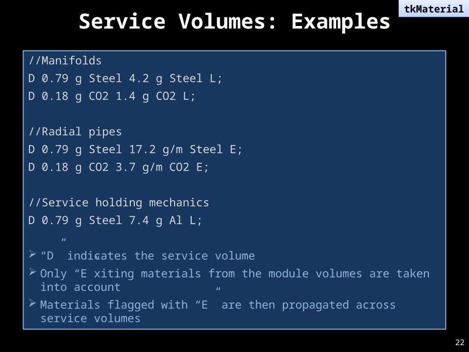
Service Volumes: ExamplestkMaterial
//Manifolds
D 0.79 g Steel 4.2 g Steel L;
D 0.18 g CO2 1.4 g CO2 L;
//Radial pipes
D 0.79 g Steel 17.2 g/m Steel E;
D 0.18 g CO2 3.7 g/m CO2 E;
//Service holding mechanics
D 0.79 g Steel 7.4 g Al L;
“D” indicates the service volume Only “E”xiting materials from the module volumes are taken into account Materials flagged with “E” are then propagated across service volumes
23
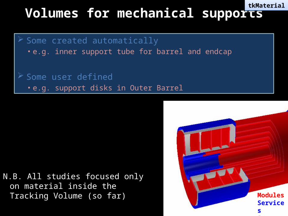
Volumes for mechanical supportstkMaterial
Some created automatically • e.g. inner support tube for barrel and endcap
Some user defined• e.g. support disks in Outer Barrel
N.B. All studies focused only on material inside the Tracking Volume (so far)
ModulesServicesSupport
24
0 1
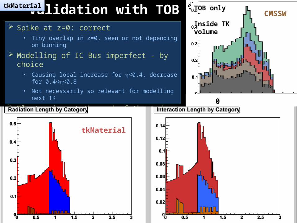
TOB only
Inside TK volume
CMSSW
Spike at z=0: correct• Tiny overlap in z=0, seen or not depending on binning
Modelling of IC Bus imperfect - by choice• Causing local increase for <0.4, decrease for 0.4<<0.8
• Not necessarily so relevant for modelling next TK
Electronics at the end of the rod (CCUM, optical connectors, wiring…) moved just outside• Makes rising edge of the peak sharper
Validation with TOBtkMaterial
tkMaterial
25
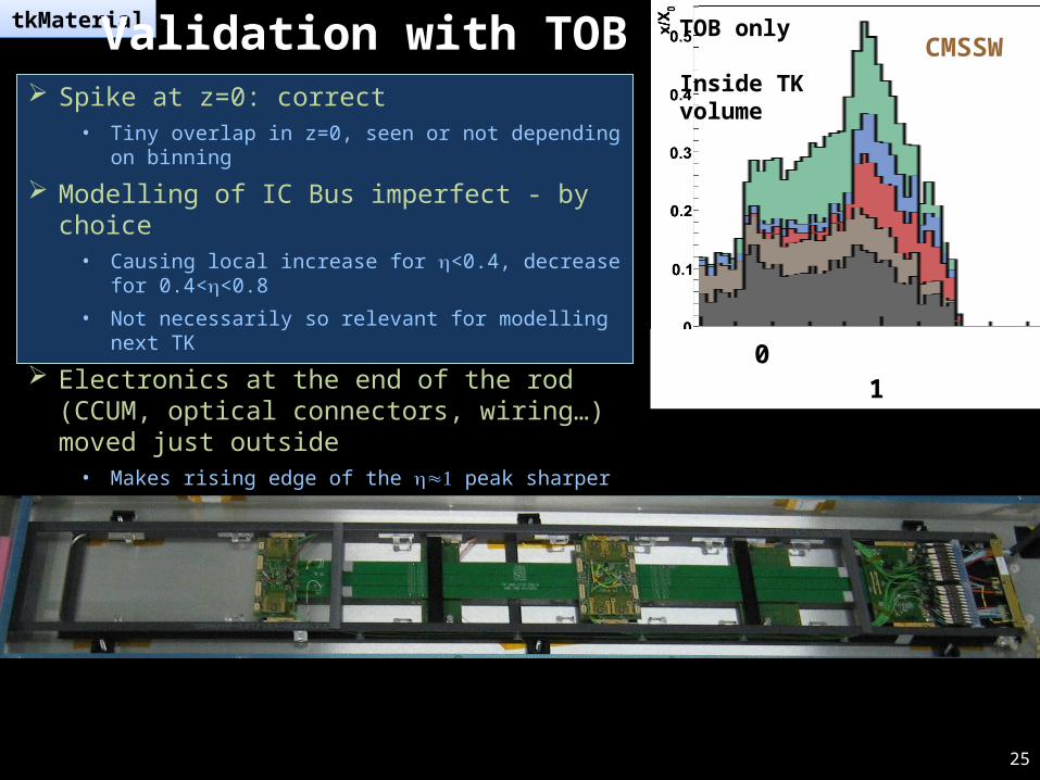
0 1
TOB only
Inside TK volume
CMSSWtkMaterial
Spike at z=0: correct• Tiny overlap in z=0, seen or not depending on binning
Modelling of IC Bus imperfect - by choice• Causing local increase for <0.4, decrease for 0.4<<0.8
• Not necessarily so relevant for modelling next TK
Electronics at the end of the rod (CCUM, optical connectors, wiring…) moved just outside• Makes rising edge of the peak sharper
Validation with TOB
26
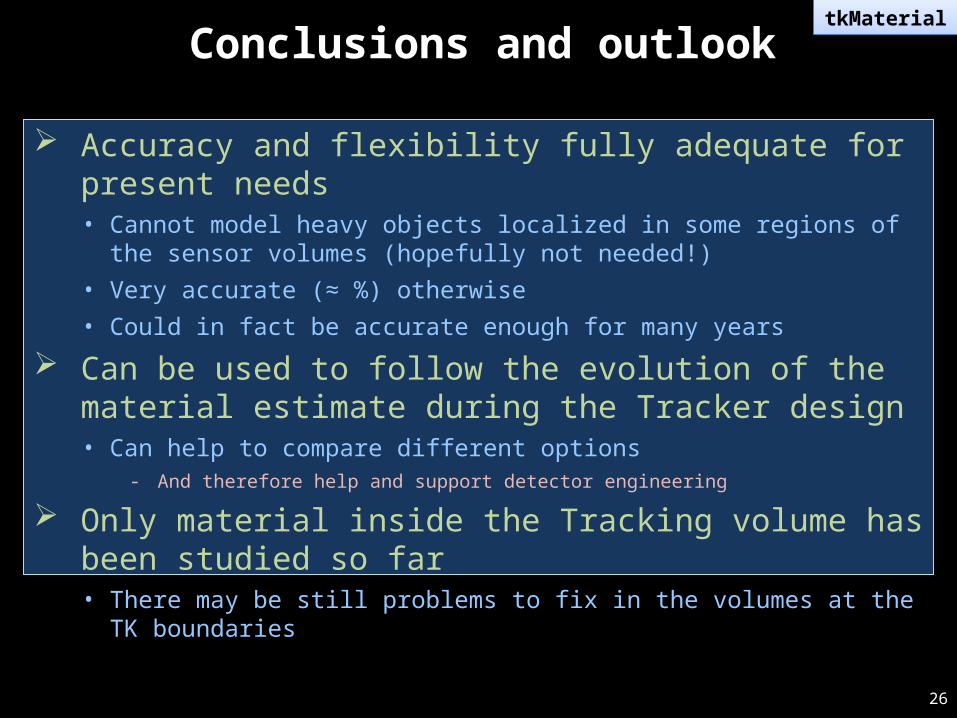
Conclusions and outlooktkMaterial
Accuracy and flexibility fully adequate for present needs• Cannot model heavy objects localized in some regions of the sensor volumes
(hopefully not needed!)• Very accurate (≈ %) otherwise• Could in fact be accurate enough for many years
Can be used to follow the evolution of the material estimate during the Tracker design• Can help to compare different options
- And therefore help and support detector engineering
Only material inside the Tracking volume has been studied so far• There may be still problems to fix in the volumes at the TK boundaries
27
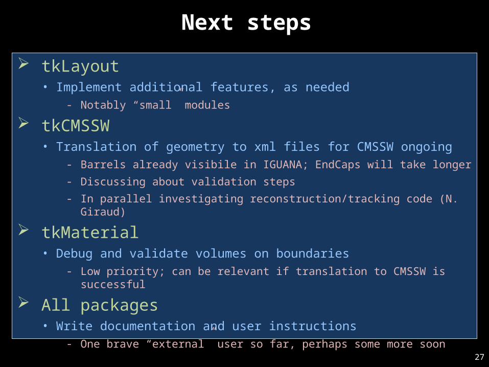
Next steps
tkLayout• Implement additional features, as needed
- Notably “small” modules
tkCMSSW• Translation of geometry to xml files for CMSSW ongoing
- Barrels already visibile in IGUANA; EndCaps will take longer- Discussing about validation steps- In parallel investigating reconstruction/tracking code (N. Giraud)
tkMaterial• Debug and validate volumes on boundaries
- Low priority; can be relevant if translation to CMSSW is successful
All packages• Write documentation and user instructions
- One brave “external” user so far, perhaps some more soon
28
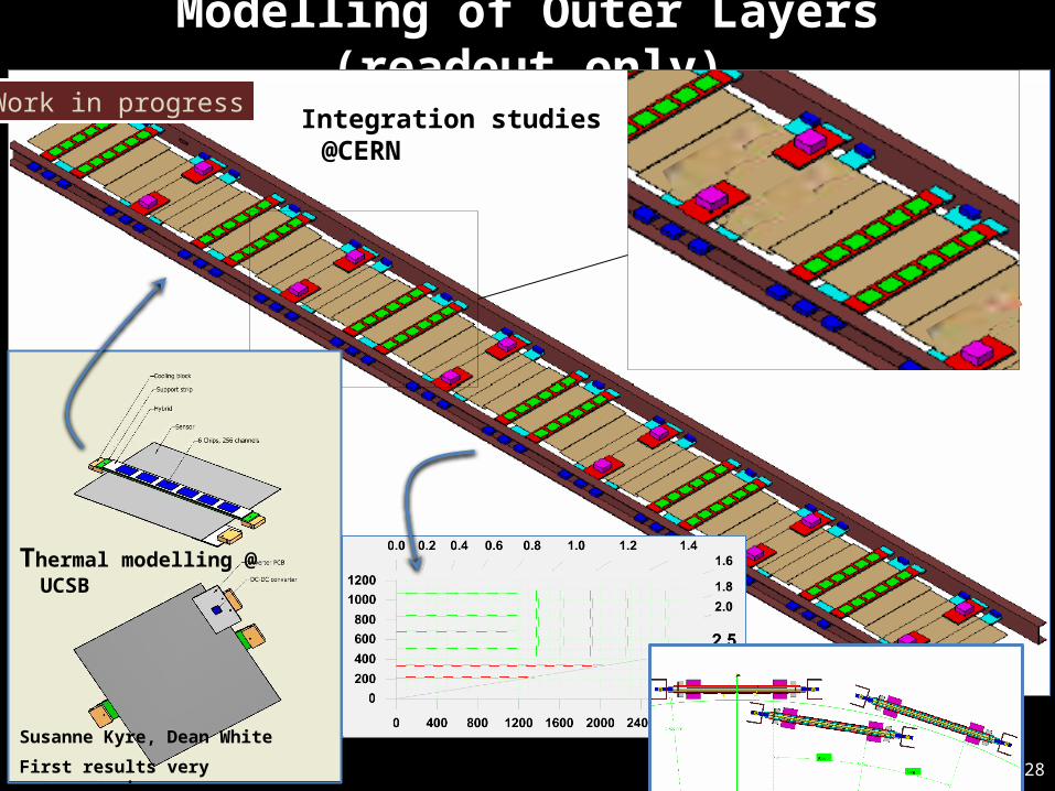
Modelling of Outer Layers (readout only)
3D design by Antonio Conde Garcia
Integration studies @CERN
Thermal modelling @ UCSB
Susanne Kyre, Dean White
First results very encouraging
Work in progress
29
General concepts(details given in previous presentations)
Strip length reduced to ≈ 5 or 2.5 cm to cope with particle density
Hybrids mounted on sensors. One hybrid serving two rows of strips
Pitch adapter integrated on hybrid (or on sensor)
Power through wires, data through twps, no large PCBs
Optical links (GBT) integrated at the end of the rods (periphery of disks)• GBTs receive twps from modules• Assume TOB twps, for the time being
Power converters integrated on small separate PCBs, one per hybrid
Mechanics and cooling contacts adapted from present TOB• Assume CO2 cooling
For material modelling take wires, connectors and all other elements from TOB• A priori pessimistic• Should ensure that nothing relevant is forgotten
30
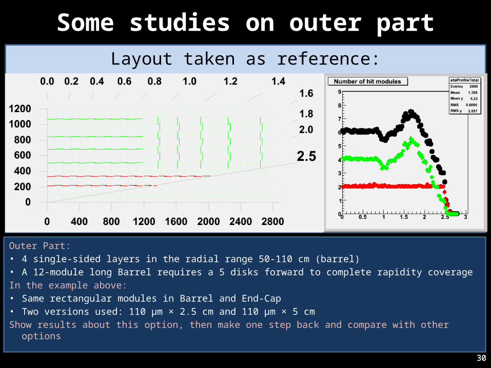
Some studies on outer partLayout taken as reference:
30
Outer Part:• 4 single-sided layers in the radial range 50-110 cm (barrel)• A 12-module long Barrel requires a 5 disks forward to complete rapidity coverageIn the example above:• Same rectangular modules in Barrel and End-Cap• Two versions used: 110 μm × 2.5 cm and 110 μm × 5 cm Show results about this option, then make one step back and compare with other options
31
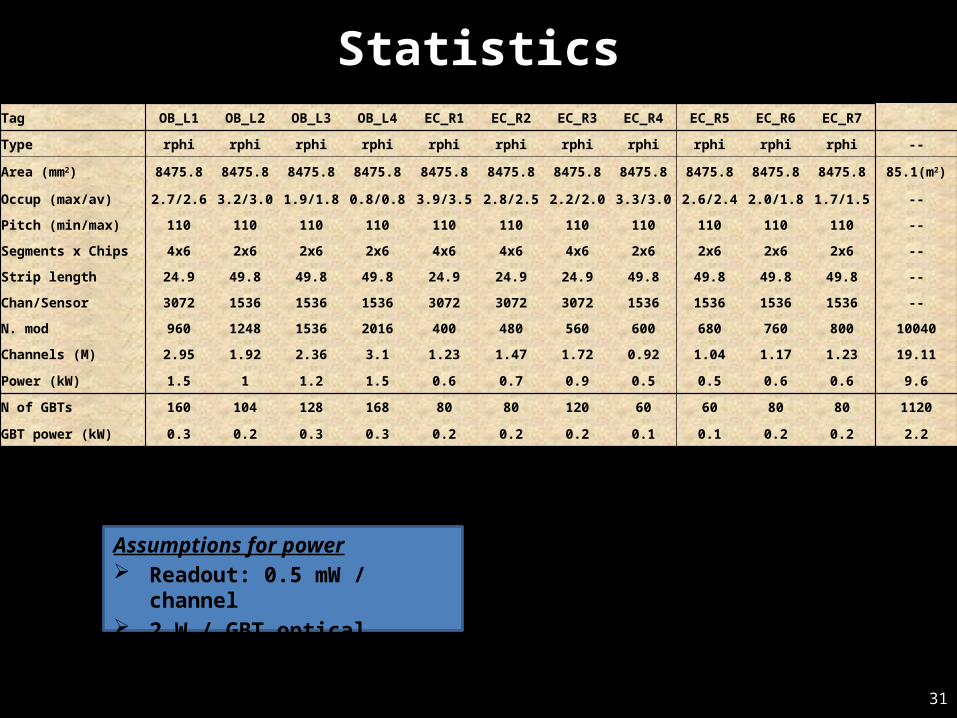
StatisticsTag OB_L1 OB_L2 OB_L3 OB_L4 EC_R1 EC_R2 EC_R3 EC_R4 EC_R5 EC_R6 EC_R7
Type rphi rphi rphi rphi rphi rphi rphi rphi rphi rphi rphi --
Area (mm2) 8475.8 8475.8 8475.8 8475.8 8475.8 8475.8 8475.8 8475.8 8475.8 8475.8 8475.8 85.1(m2)
Occup (max/av) 2.7/2.6 3.2/3.0 1.9/1.8 0.8/0.8 3.9/3.5 2.8/2.5 2.2/2.0 3.3/3.0 2.6/2.4 2.0/1.8 1.7/1.5 --
Pitch (min/max) 110 110 110 110 110 110 110 110 110 110 110 --
Segments x Chips 4x6 2x6 2x6 2x6 4x6 4x6 4x6 2x6 2x6 2x6 2x6 --
Strip length 24.9 49.8 49.8 49.8 24.9 24.9 24.9 49.8 49.8 49.8 49.8 --
Chan/Sensor 3072 1536 1536 1536 3072 3072 3072 1536 1536 1536 1536 --
N. mod 960 1248 1536 2016 400 480 560 600 680 760 800 10040
Channels (M) 2.95 1.92 2.36 3.1 1.23 1.47 1.72 0.92 1.04 1.17 1.23 19.11
Power (kW) 1.5 1 1.2 1.5 0.6 0.7 0.9 0.5 0.5 0.6 0.6 9.6
N of GBTs 160 104 128 168 80 80 120 60 60 80 80 1120
GBT power (kW) 0.3 0.2 0.3 0.3 0.2 0.2 0.2 0.1 0.1 0.2 0.2 2.2
Assumptions for power Readout: 0.5 mW / channel 2 W / GBT optical channel
32
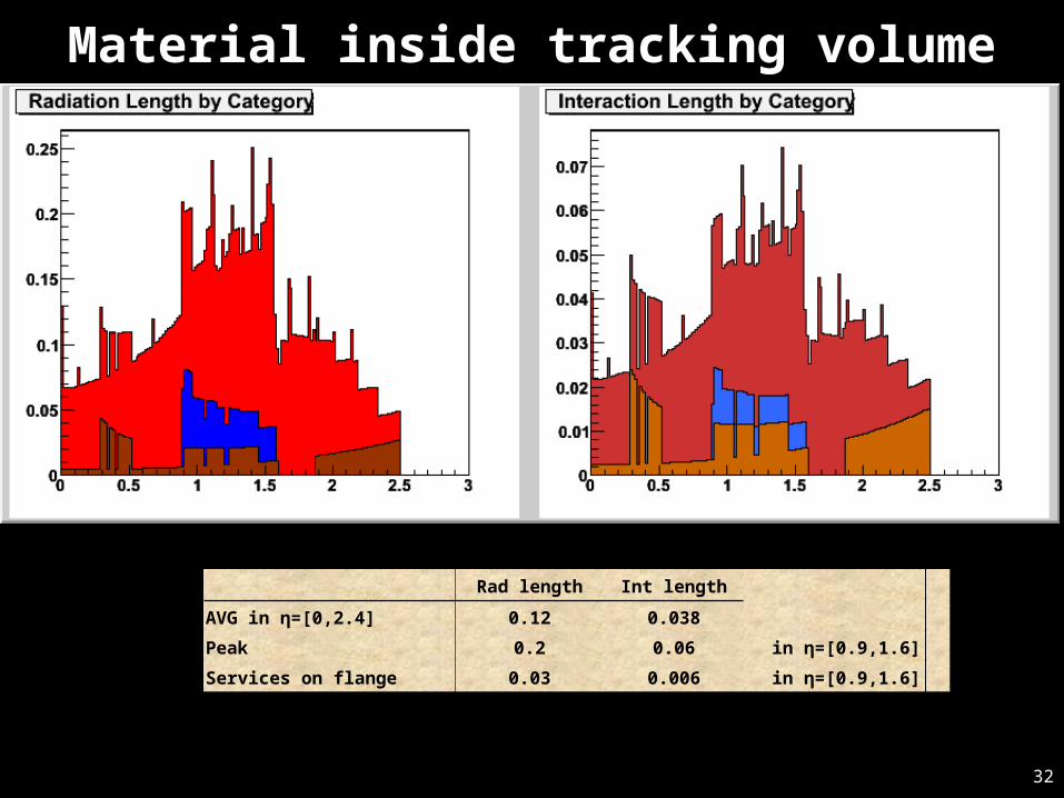
Material inside tracking volume
Rad length Int length
AVG in η=[0,2.4] 0.12 0.038
Peak 0.2 0.06 in η=[0.9,1.6]
Services on flange 0.03 0.006 in η=[0.9,1.6]
33
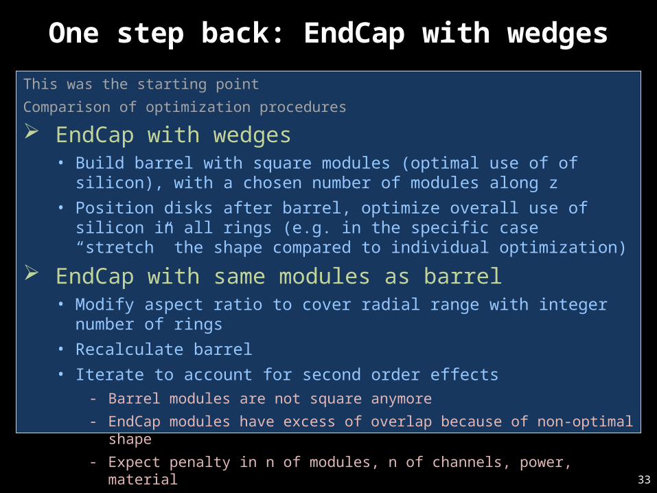
One step back: EndCap with wedgesThis was the starting point
Comparison of optimization procedures
EndCap with wedges• Build barrel with square modules (optimal use of of silicon), with a chosen number
of modules along z• Position disks after barrel, optimize overall use of silicon in all rings (e.g. in the
specific case “stretch” the shape compared to individual optimization)
EndCap with same modules as barrel• Modify aspect ratio to cover radial range with integer number of rings• Recalculate barrel• Iterate to account for second order effects
- Barrel modules are not square anymore- EndCap modules have excess of overlap because of non-optimal shape- Expect penalty in n of modules, n of channels, power, material
34
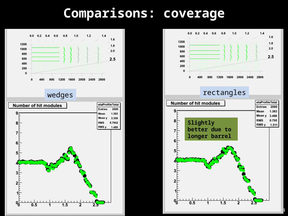
Comparisons: coverage
wedges rectangles
Slightly better due to longer barrel
35
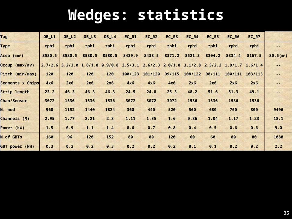
Wedges: statisticsTag OB_L1 OB_L2 OB_L3 OB_L4 EC_R1 EC_R2 EC_R3 EC_R4 EC_R5 EC_R6 EC_R7
Type rphi rphi rphi rphi rphi rphi rphi rphi rphi rphi rphi --
Area (mm2) 8580.5 8580.5 8580.5 8580.5 8439.9 8438.5 8371.2 8521.3 8304.2 8334.4 8167.5 80.5(m2)
Occup (max/av) 2.7/2.6 3.2/3.0 1.8/1.8 0.9/0.8 3.5/3.1 2.6/2.3 2.0/1.8 3.1/2.8 2.5/2.2 1.9/1.7 1.6/1.4 --
Pitch (min/max) 120 120 120 120 100/123 101/120 99/115 108/122 98/111 100/111 103/113 --
Segments x Chips 4x6 2x6 2x6 2x6 4x6 4x6 4x6 2x6 2x6 2x6 2x6 --
Strip length 23.2 46.3 46.3 46.3 24.5 24.8 25.3 48.2 51.6 51.3 49.1 --
Chan/Sensor 3072 1536 1536 1536 3072 3072 3072 1536 1536 1536 1536 --
N. mod 960 1152 1440 1824 360 440 520 560 680 760 800 9496
Channels (M) 2.95 1.77 2.21 2.8 1.11 1.35 1.6 0.86 1.04 1.17 1.23 18.1
Power (kW) 1.5 0.9 1.1 1.4 0.6 0.7 0.8 0.4 0.5 0.6 0.6 9.0
N of GBTs 160 96 120 152 80 80 120 60 60 80 80 1088
GBT power (kW) 0.3 0.2 0.2 0.3 0.2 0.2 0.2 0.1 0.1 0.2 0.2 2.2
36
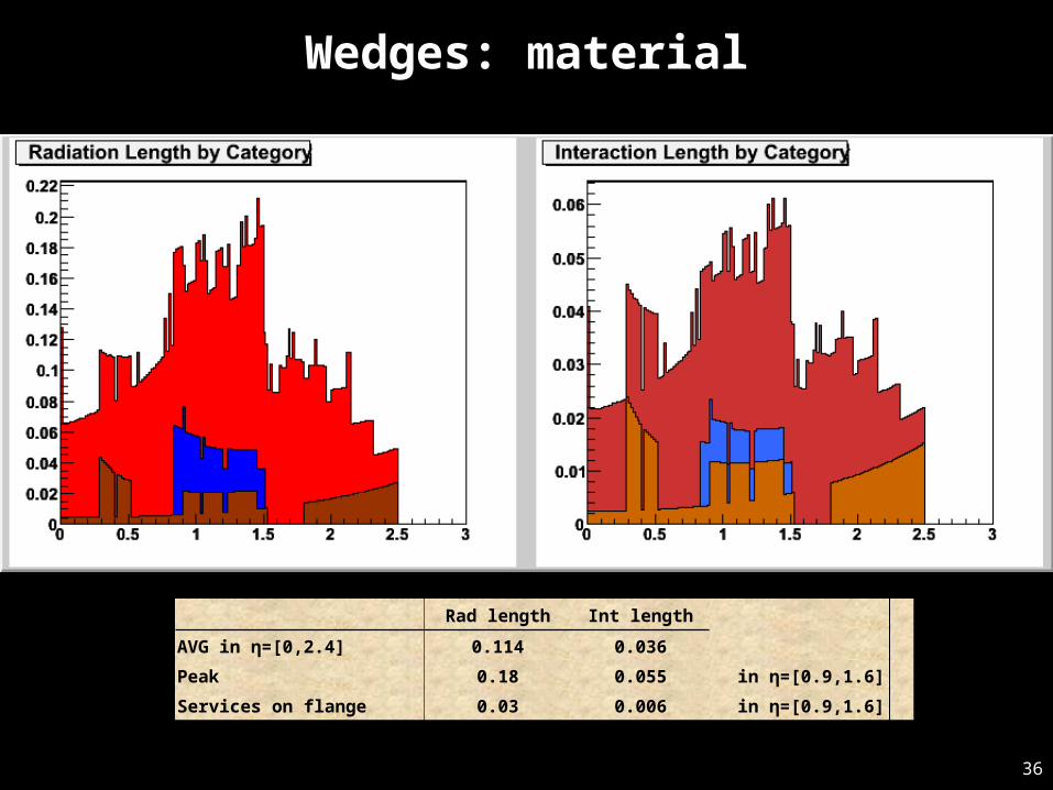
Wedges: material
Rad length Int length
AVG in η=[0,2.4] 0.114 0.036
Peak 0.18 0.055 in η=[0.9,1.6]
Services on flange 0.03 0.006 in η=[0.9,1.6]
37
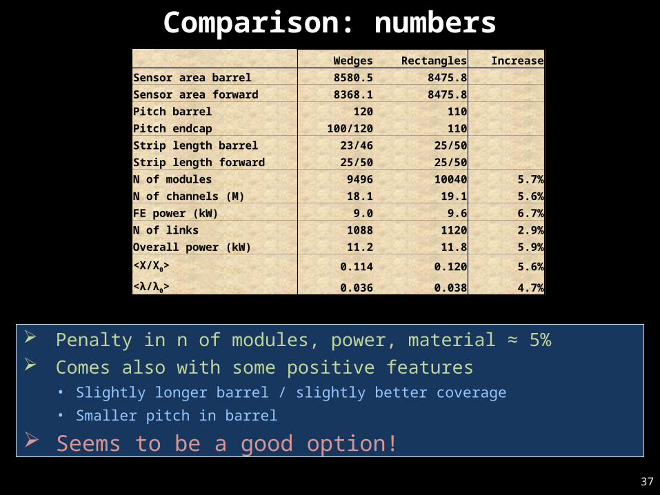
Comparison: numbers
Penalty in n of modules, power, material ≈ 5% Comes also with some positive features
• Slightly longer barrel / slightly better coverage• Smaller pitch in barrel
Seems to be a good option!
Wedges Rectangles Increase
Sensor area barrel 8580.5 8475.8
Sensor area forward 8368.1 8475.8
Pitch barrel 120 110
Pitch endcap 100/120 110
Strip length barrel 23/46 25/50
Strip length forward 25/50 25/50
N of modules 9496 10040 5.7%
N of channels (M) 18.1 19.1 5.6%
FE power (kW) 9.0 9.6 6.7%
N of links 1088 1120 2.9%
Overall power (kW) 11.2 11.8 5.9%
<X/X0> 0.114 0.120 5.6%
<λ/λ0> 0.036 0.038 4.7%
38
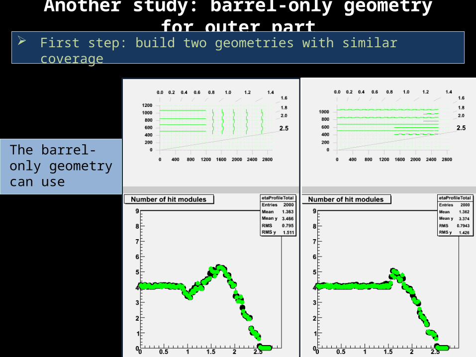
Another study: barrel-only geometry for outer part First step: build two geometries with similar coverage
The barrel-only geometry can use square detectors
39
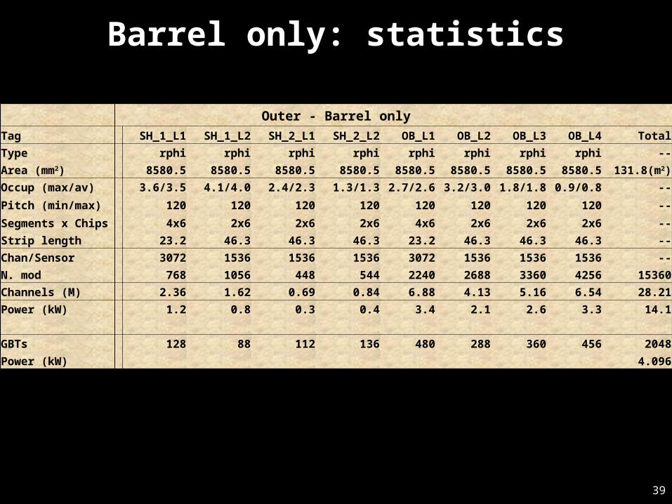
Barrel only: statistics
Outer - Barrel only
Tag SH_1_L1 SH_1_L2 SH_2_L1 SH_2_L2 OB_L1 OB_L2 OB_L3 OB_L4 Total
Type rphi rphi rphi rphi rphi rphi rphi rphi --
Area (mm2) 8580.5 8580.5 8580.5 8580.5 8580.5 8580.5 8580.5 8580.5 131.8(m2)
Occup (max/av) 3.6/3.5 4.1/4.0 2.4/2.3 1.3/1.3 2.7/2.6 3.2/3.0 1.8/1.8 0.9/0.8 --
Pitch (min/max) 120 120 120 120 120 120 120 120 --
Segments x Chips 4x6 2x6 2x6 2x6 4x6 2x6 2x6 2x6 --
Strip length 23.2 46.3 46.3 46.3 23.2 46.3 46.3 46.3 --
Chan/Sensor 3072 1536 1536 1536 3072 1536 1536 1536 --
N. mod 768 1056 448 544 2240 2688 3360 4256 15360
Channels (M) 2.36 1.62 0.69 0.84 6.88 4.13 5.16 6.54 28.21
Power (kW) 1.2 0.8 0.3 0.4 3.4 2.1 2.6 3.3 14.1
GBTs 128 88 112 136 480 288 360 456 2048
Power (kW) 4.096
40
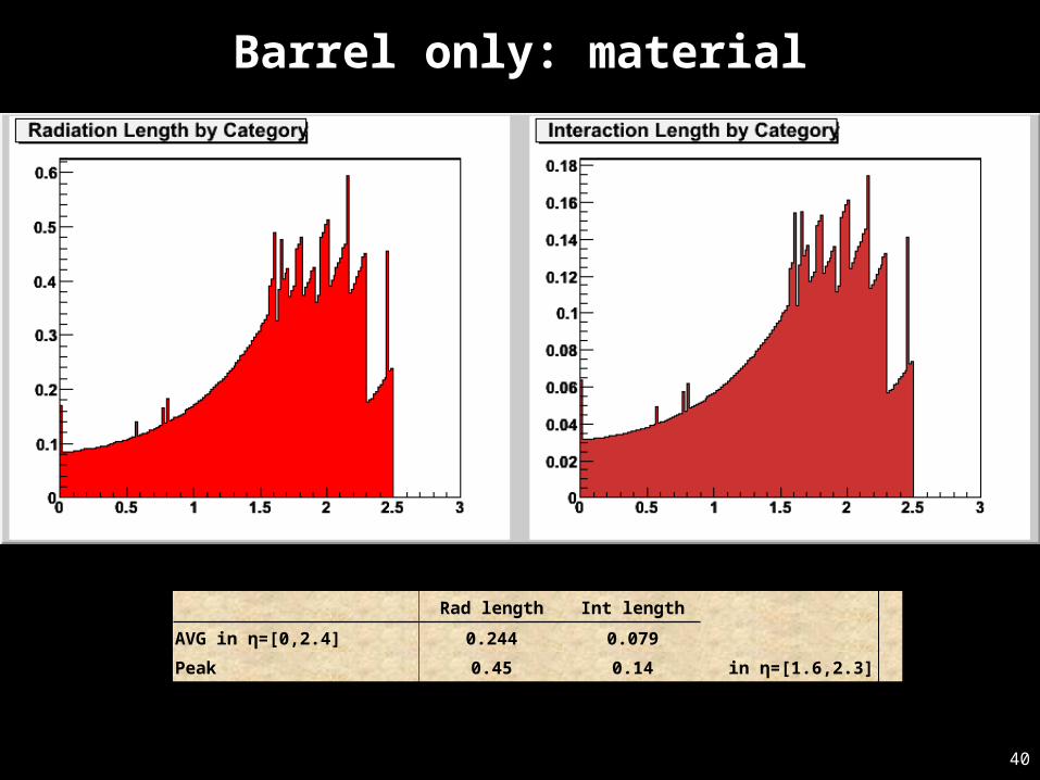
Barrel only: material
Rad length Int length
AVG in η=[0,2.4] 0.244 0.079
Peak 0.45 0.14 in η=[1.6,2.3]
41
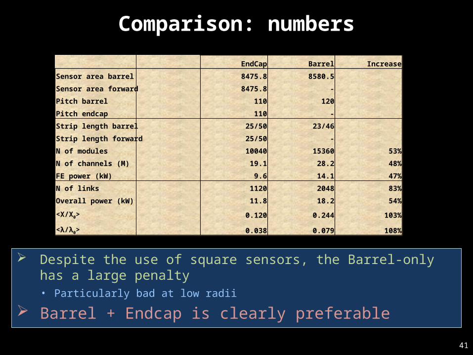
Comparison: numbersEndCap Barrel Increase
Sensor area barrel 8475.8 8580.5
Sensor area forward 8475.8 -
Pitch barrel 110 120
Pitch endcap 110 -
Strip length barrel 25/50 23/46
Strip length forward 25/50 -
N of modules 10040 15360 53%
N of channels (M) 19.1 28.2 48%
FE power (kW) 9.6 14.1 47%
N of links 1120 2048 83%
Overall power (kW) 11.8 18.2 54%
<X/X0> 0.120 0.244 103%
<λ/λ0> 0.038 0.079 108%
Despite the use of square sensors, the Barrel-only has a large penalty• Particularly bad at low radii
Barrel + Endcap is clearly preferable
42
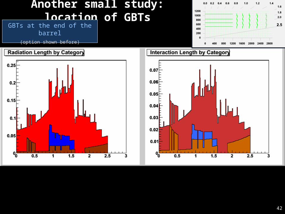
Another small study: location of GBTsGBTs at the end of the barrel
(option shown before)
43
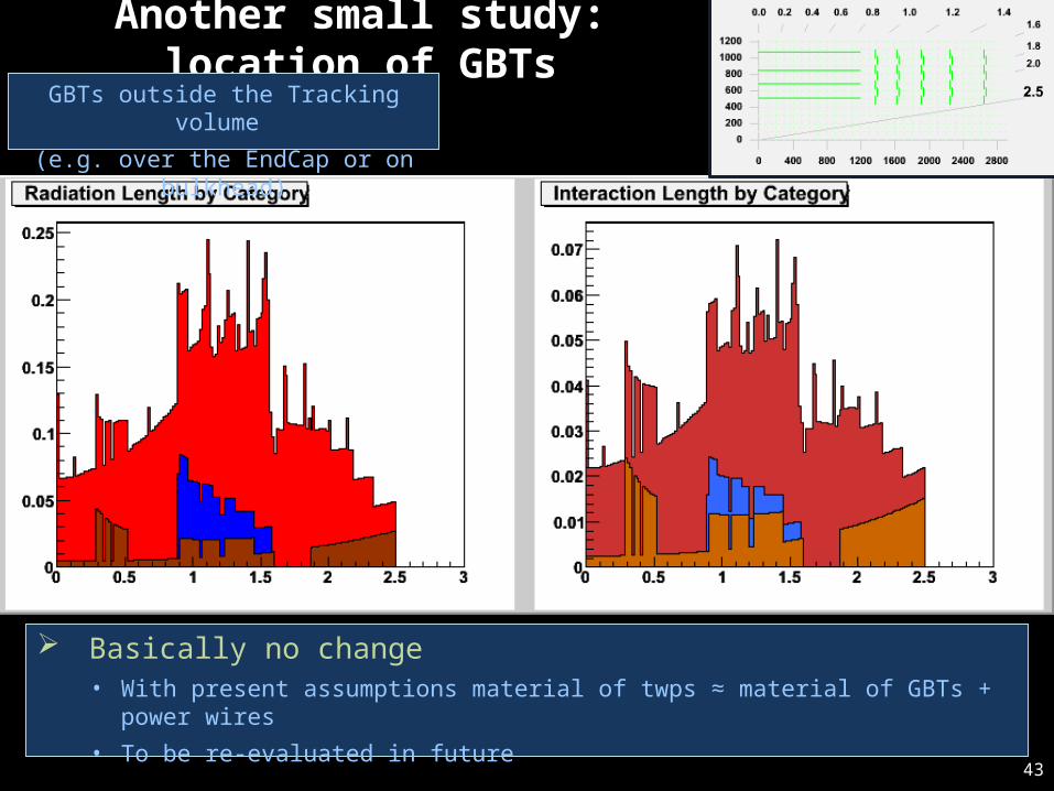
Basically no change• With present assumptions material of twps ≈ material of GBTs + power wires• To be re-evaluated in future
Another small study: location of GBTsGBTs outside the Tracking volume
(e.g. over the EndCap or on bulkhead)
44
Next step: modelling of PT layers
Understanding of integration aspects much more limited than for readout layers• Dedicated discussion in TUPO last week• Expect more progress in the coming weeks/months
Used as baseline the two geometries presented in the R&D proposal from Geoff/Anders• Surface similar, module material similar, power estimates compatible,
data rate the same (given by functionality)- No need to distinguish between the two at this stage
Part list should be reasonably OK• Although it is not yet understood how they may come together• Some provision of material for cooling (and mechanics)• Basic assumptions recalled in the following slides
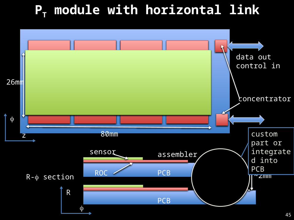
PT module with horizontal link
45
concentrator
sensor
ROC
assembler
PCB
PCB
~2mmR-f section
80mm
data outcontrol in
26mm
f
z
f
R
custom part or integrated into PCB
46
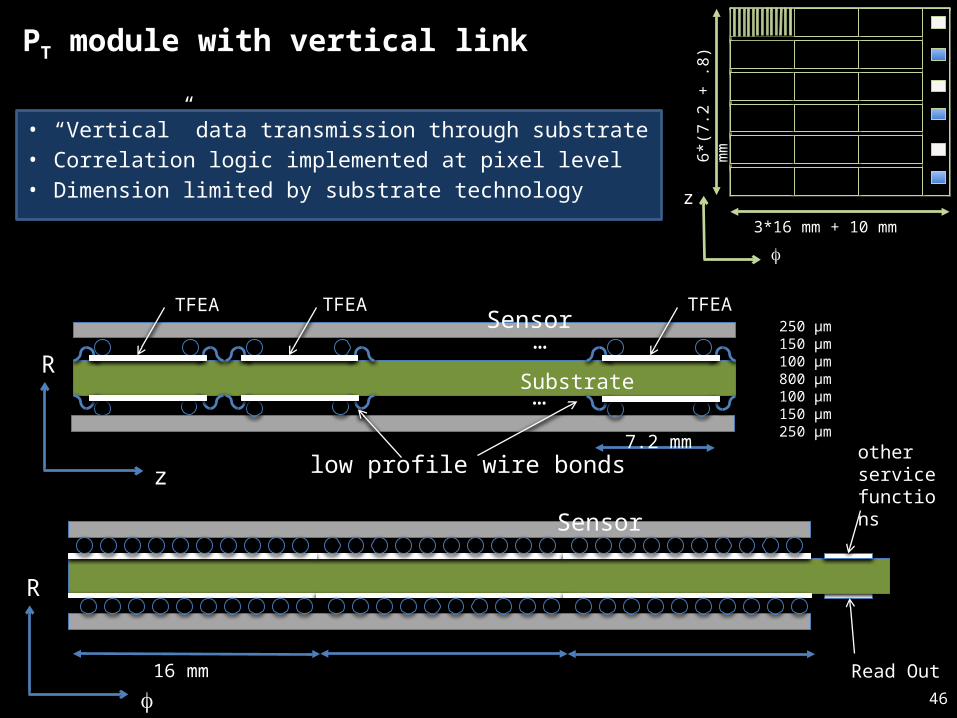
PT module with vertical link
Read Out16 mm
other service functions
f
R
Sensor
250 μm150 μm100 μm800 μm100 μm150 μm250 μm
Substrate
…
…
7.2 mm
TFEA TFEA TFEA
z
R
Sensor
low profile wire bonds
6*(7
.2 +
.8) m
m
3*16 mm + 10 mm
f
z
• “Vertical” data transmission through substrate• Correlation logic implemented at pixel level• Dimension limited by substrate technology
47
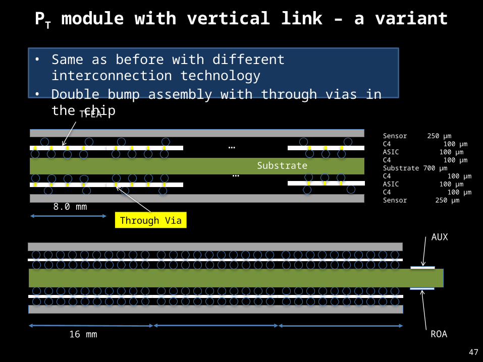
PT module with vertical link – a variant
ROA16 mm
AUX
Sensor 250 μmC4 100 μmASIC 100 μmC4 100 μmSubstrate 700 μmC4 100 μmASIC 100 μmC4 100 μmSensor 250 μm
8.0 mm
TFEA
Substrate
…
…
Through Via
• Same as before with different interconnection technology• Double bump assembly with through vias in the chip
48
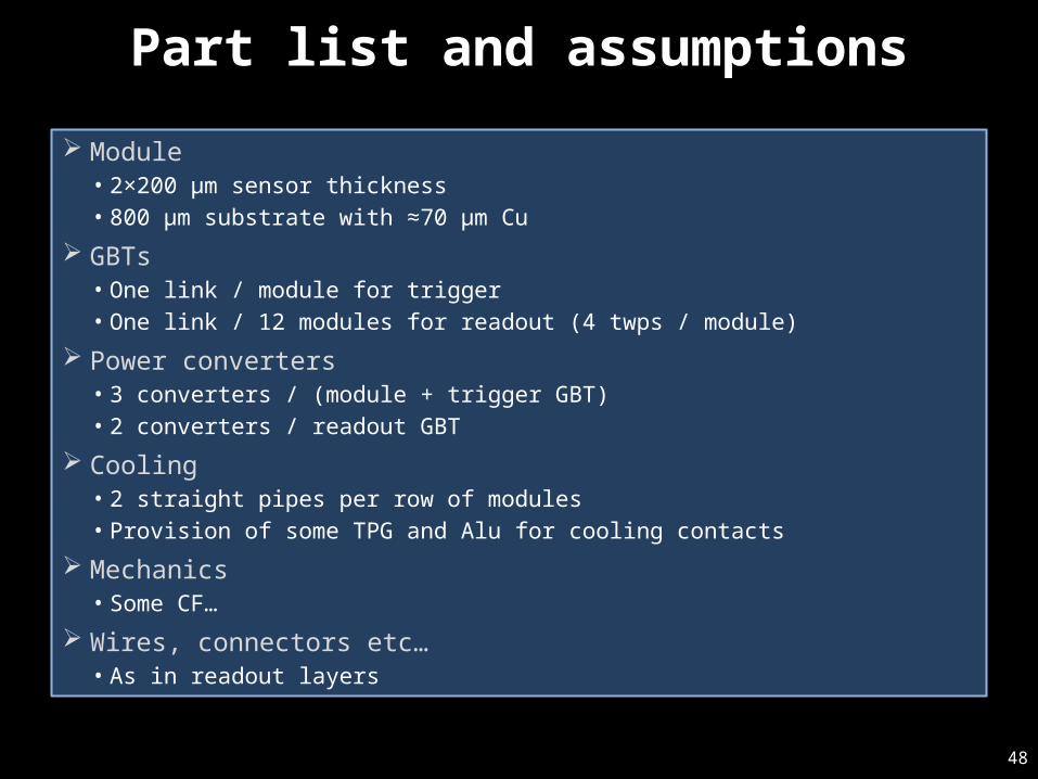
Part list and assumptions
Module• 2×200 μm sensor thickness• 800 μm substrate with ≈70 μm Cu
GBTs• One link / module for trigger• One link / 12 modules for readout (4 twps / module)
Power converters• 3 converters / (module + trigger GBT)• 2 converters / readout GBT
Cooling • 2 straight pipes per row of modules• Provision of some TPG and Alu for cooling contacts
Mechanics• Some CF…
Wires, connectors etc…• As in readout layers
49
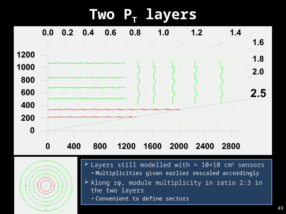
Two PT layers
Layers still modelled with ≈ 10×10 cm2 sensors• Multiplicities given earlier rescaled accordingly
Along rϕ, module multiplicity in ratio 2:3 in the two layers• Convenient to define sectors
50
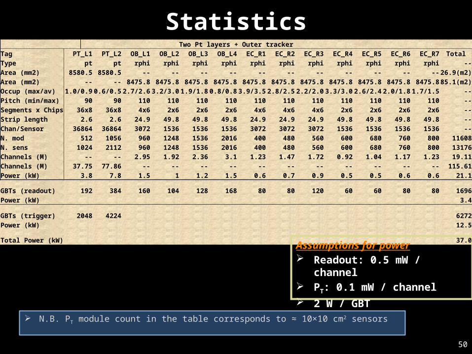
Statistics
N.B. PT module count in the table corresponds to ≈ 10×10 cm2 sensors
Two Pt layers + Outer trackerTag PT_L1 PT_L2 OB_L1 OB_L2 OB_L3 OB_L4 EC_R1 EC_R2 EC_R3 EC_R4 EC_R5 EC_R6 EC_R7 TotalType pt pt rphi rphi rphi rphi rphi rphi rphi rphi rphi rphi rphi --Area (mm2) 8580.5 8580.5 -- -- -- -- -- -- -- -- -- -- -- 26.9(m2)Area (mm2) -- -- 8475.8 8475.8 8475.8 8475.8 8475.8 8475.8 8475.8 8475.8 8475.8 8475.8 8475.8 85.1(m2)Occup (max/av) 1.0/0.9 0.6/0.5 2.7/2.6 3.2/3.0 1.9/1.8 0.8/0.8 3.9/3.5 2.8/2.5 2.2/2.0 3.3/3.0 2.6/2.4 2.0/1.8 1.7/1.5 --Pitch (min/max) 90 90 110 110 110 110 110 110 110 110 110 110 110 --Segments x Chips 36x8 36x8 4x6 2x6 2x6 2x6 4x6 4x6 4x6 2x6 2x6 2x6 2x6 --Strip length 2.6 2.6 24.9 49.8 49.8 49.8 24.9 24.9 24.9 49.8 49.8 49.8 49.8 --Chan/Sensor 36864 36864 3072 1536 1536 1536 3072 3072 3072 1536 1536 1536 1536 --N. mod 512 1056 960 1248 1536 2016 400 480 560 600 680 760 800 11608N. sens 1024 2112 960 1248 1536 2016 400 480 560 600 680 760 800 13176Channels (M) -- -- 2.95 1.92 2.36 3.1 1.23 1.47 1.72 0.92 1.04 1.17 1.23 19.11Channels (M) 37.75 77.86 -- -- -- -- -- -- -- -- -- -- -- 115.61Power (kW) 3.8 7.8 1.5 1 1.2 1.5 0.6 0.7 0.9 0.5 0.5 0.6 0.6 21.1
GBTs (readout) 192 384 160 104 128 168 80 80 120 60 60 80 80 1696Power (kW) 3.4
GBTs (trigger) 2048 4224 6272Power (kW) 12.5
Total Power (kW) 37.0
Assumptions for power Readout: 0.5 mW / channel PT: 0.1 mW / channel 2 W / GBT
51
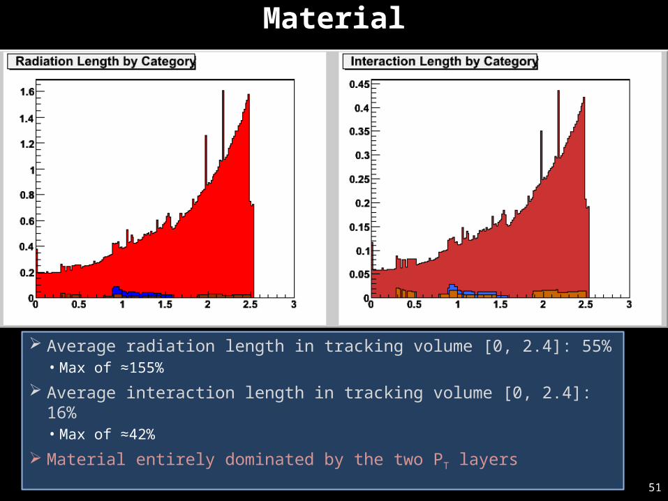
Material
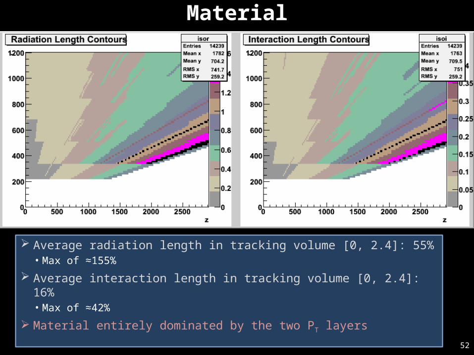
Average radiation length in tracking volume [0, 2.4]: 55%• Max of ≈155%
Average interaction length in tracking volume [0, 2.4]: 16%• Max of ≈42%
Material entirely dominated by the two PT layers
52
Material
Average radiation length in tracking volume [0, 2.4]: 55%• Max of ≈155%
Average interaction length in tracking volume [0, 2.4]: 16%• Max of ≈42%
Material entirely dominated by the two PT layers
53
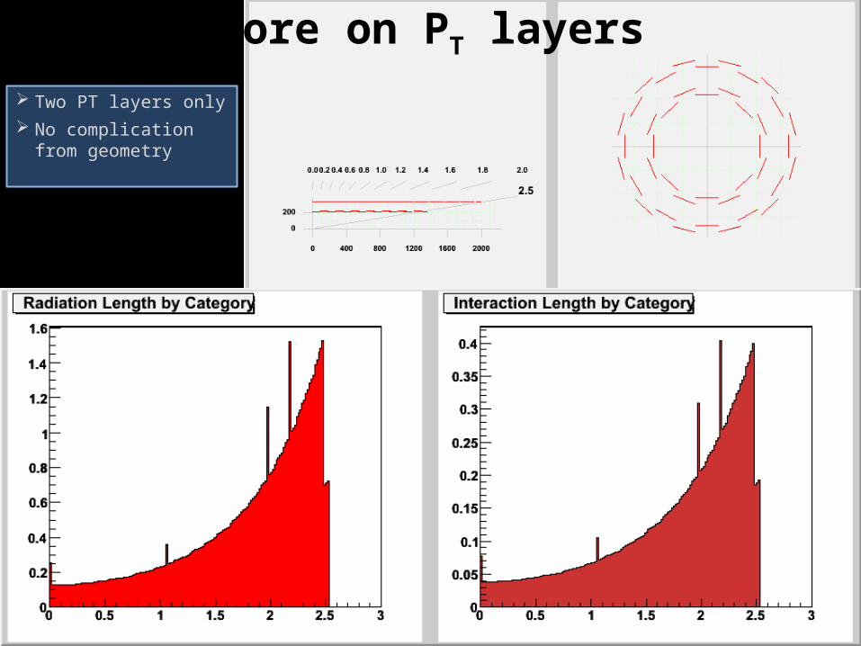
More on PT layers Two PT layers only No complication
from geometry
54
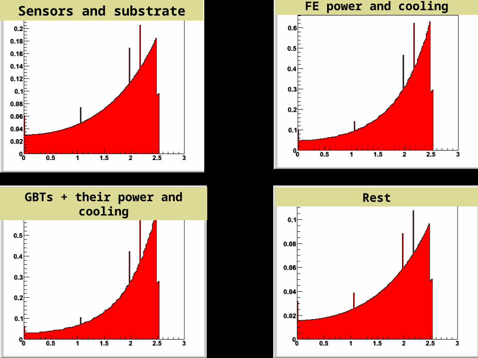
FE power and coolingSensors and substrate
GBTs + their power and cooling Rest
55
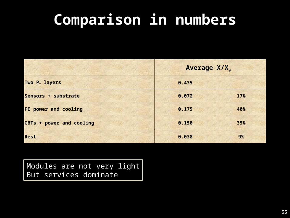
Comparison in numbers
Average X/X0
Two PT layers 0.435
Sensors + substrate 0.072 17%
FE power and cooling 0.175 40%
GBTs + power and cooling 0.150 35%
Rest 0.038 9%
Modules are not very lightBut services dominate
56
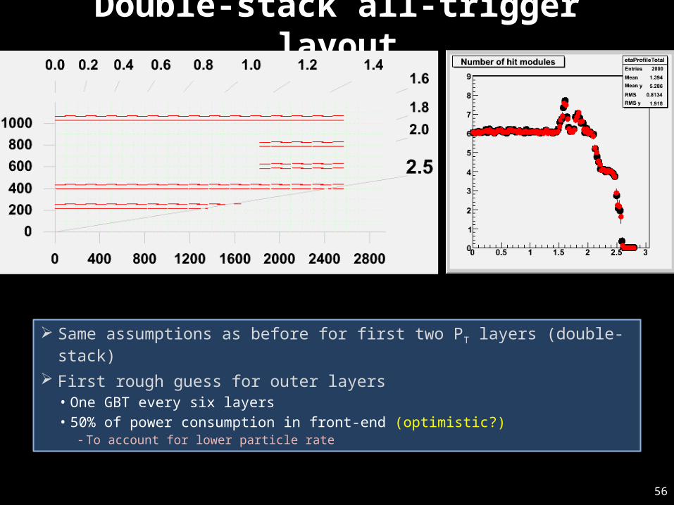
Double-stack all-trigger layout
Same assumptions as before for first two PT layers (double-stack)
First rough guess for outer layers• One GBT every six layers• 50% of power consumption in front-end (optimistic?)
- To account for lower particle rate
57
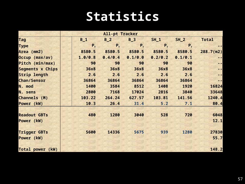
StatisticsAll-pt Tracker
Tag B_1 B_2 B_3 SH_1 SH_2 TotalType PT PT PT PT PT --Area (mm2) 8580.5 8580.5 8580.5 8580.5 8580.5 288.7(m2)Occup (max/av) 1.0/0.8 0.4/0.4 0.1/0.0 0.2/0.2 0.1/0.1 --Pitch (min/max) 90 90 90 90 90 --Segments x Chips 36x8 36x8 36x8 36x8 36x8 --Strip length 2.6 2.6 2.6 2.6 2.6 --Chan/Sensor 36864 36864 36864 36864 36864 --N. mod 1400 3584 8512 1408 1920 16824N. sens 2800 7168 17024 2816 3840 33648Channels (M) 103.22 264.24 627.57 103.81 141.56 1240.4Power (kW) 10.3 26.4 31.4 5.2 7.1 80.4
Readout GBTs 480 1280 3040 528 720 6048Power (kW) 12.1
Trigger GBTs 5600 14336 5675 939 1280 27830Power (kW) 55.7
Total power (kW) 148.2
58
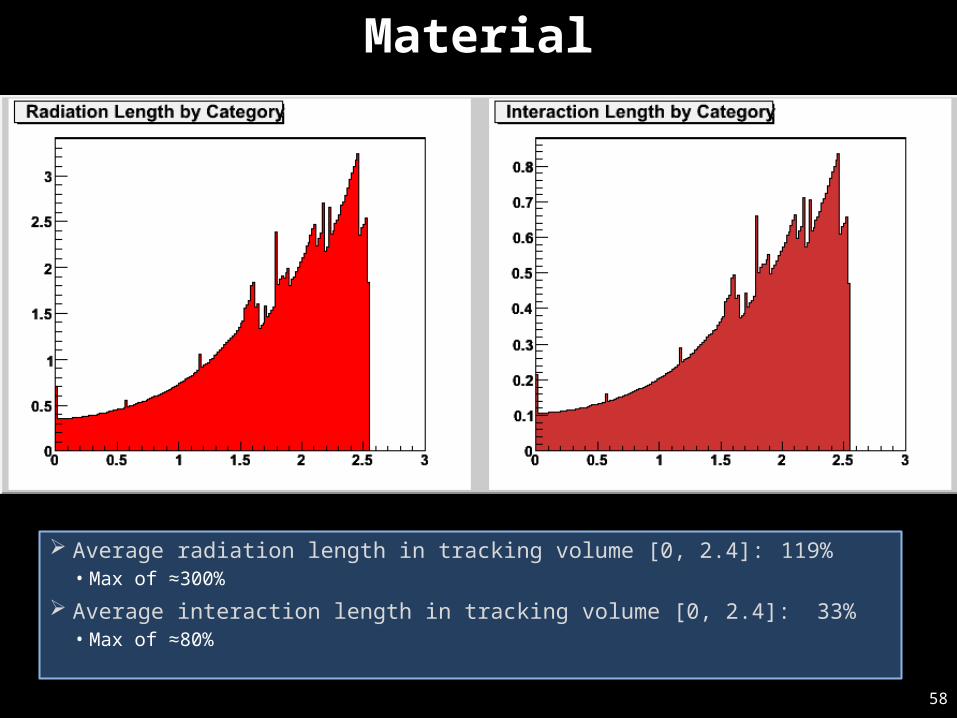
Material
Average radiation length in tracking volume [0, 2.4]: 119%• Max of ≈300%
Average interaction length in tracking volume [0, 2.4]: 33%• Max of ≈80%
59
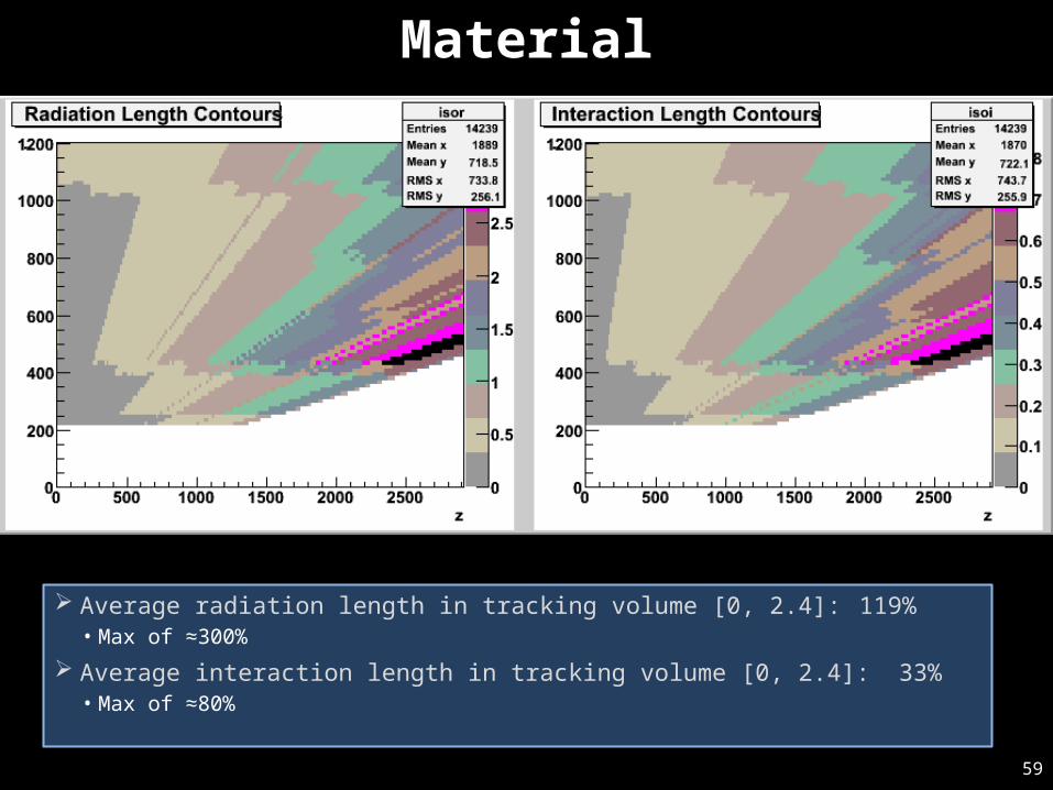
Material
Average radiation length in tracking volume [0, 2.4]: 119%• Max of ≈300%
Average interaction length in tracking volume [0, 2.4]: 33%• Max of ≈80%
60
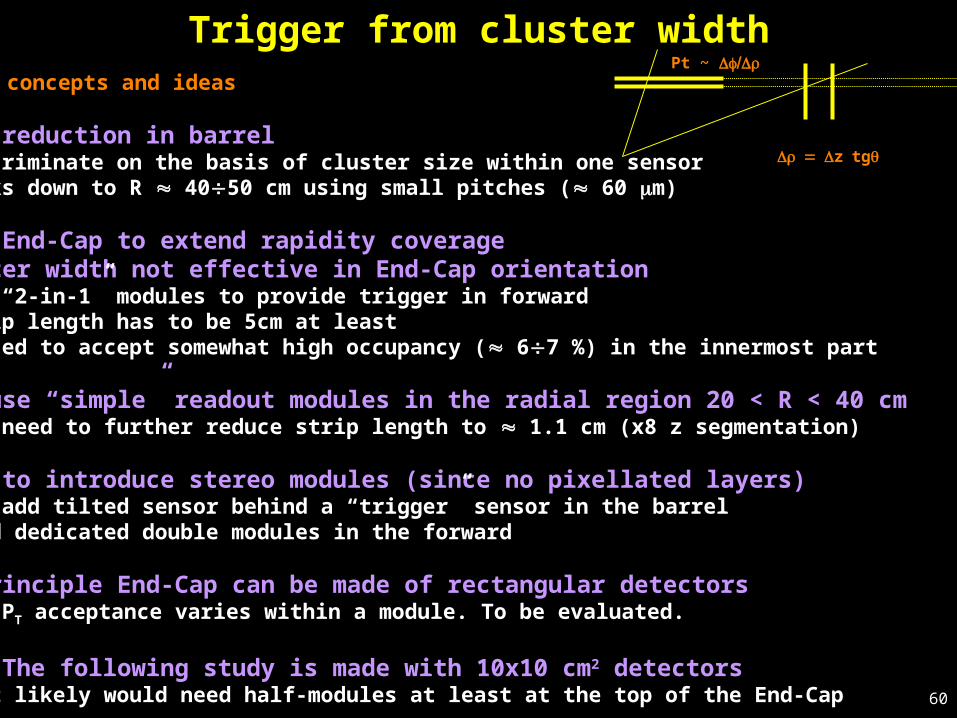
Basic concepts and ideas
Data reduction in barrel• Discriminate on the basis of cluster size within one sensor• Works down to R 4050 cm using small pitches ( 60 m)
Need End-Cap to extend rapidity coverageCluster width not effective in End-Cap orientation • Use “2-in-1” modules to provide trigger in forward• Strip length has to be 5cm at least• Forced to accept somewhat high occupancy ( 67 %) in the innermost part
Can use “simple” readout modules in the radial region 20 < R < 40 cm• But need to further reduce strip length to 1.1 cm (x8 z segmentation)
Need to introduce stereo modules (since no pixellated layers)• Can add tilted sensor behind a “trigger” sensor in the barrel• Need dedicated double modules in the forward
In principle End-Cap can be made of rectangular detectors• But PT acceptance varies within a module. To be evaluated.
N.B. The following study is made with 10x10 cm2 detectors• Most likely would need half-modules at least at the top of the End-Cap
Trigger from cluster widthPt ~
ztg
61
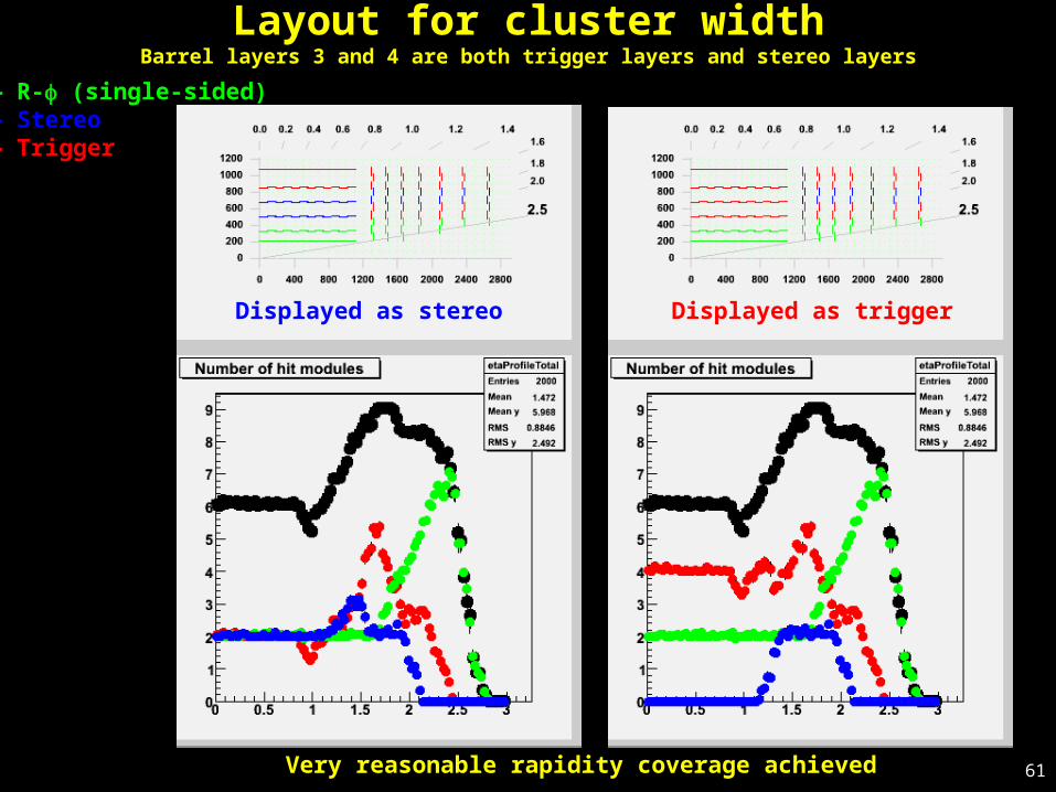
Layout for cluster widthBarrel layers 3 and 4 are both trigger layers and stereo layers
Displayed as stereo Displayed as trigger
— R- (single-sided)— Stereo— Trigger
Very reasonable rapidity coverage achieved
62
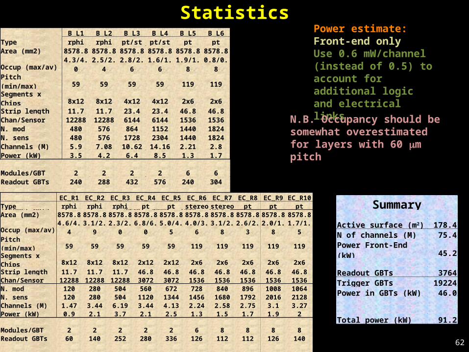
StatisticsPower estimate:Front-end onlyUse 0.6 mW/channel (instead of 0.5) to account for additional logic and electrical links
N.B. Occupancy should be somewhat overestimated for layers with 60 m pitch
B_L1 B_L2 B_L3 B_L4 B_L5 B_L6Type rphi rphi pt/st pt/st pt ptArea (mm2) 8578.8 8578.8 8578.8 8578.8 8578.8 8578.8Occup (max/av) 4.3/4.0 2.5/2.4 2.8/2.6 1.6/1.6 1.9/1.8 0.8/0.8Pitch (min/max) 59 59 59 59 119 119Segments x Chips 8x12 8x12 4x12 4x12 2x6 2x6Strip length 11.7 11.7 23.4 23.4 46.8 46.8Chan/Sensor 12288 12288 6144 6144 1536 1536N. mod 480 576 864 1152 1440 1824N. sens 480 576 1728 2304 1440 1824Channels (M) 5.9 7.08 10.62 14.16 2.21 2.8Power (kW) 3.5 4.2 6.4 8.5 1.3 1.7
Modules/GBT 2 2 2 2 6 6Readout GBTs 240 288 432 576 240 304
GBTs/module 4 4 1 1Trigger GBTs 3456 4608 1440 1824
EC_R1 EC_R2 EC_R3 EC_R4 EC_R5 EC_R6 EC_R7 EC_R8 EC_R9 EC_R10Type rphi rphi rphi pt pt stereo stereo pt pt ptArea (mm2) 8578.8 8578.8 8578.8 8578.8 8578.8 8578.8 8578.8 8578.8 8578.8 8578.8Occup (max/av) 4.6/4.4 3.1/2.9 2.3/2.0 6.8/6.0 5.0/4.5 4.0/3.6 3.1/2.8 2.6/2.3 2.0/1.8 1.7/1.5Pitch (min/max) 59 59 59 59 59 119 119 119 119 119Segments x Chips 8x12 8x12 8x12 2x12 2x12 2x6 2x6 2x6 2x6 2x6Strip length 11.7 11.7 11.7 46.8 46.8 46.8 46.8 46.8 46.8 46.8Chan/Sensor 12288 12288 12288 3072 3072 1536 1536 1536 1536 1536N. mod 120 280 504 560 672 728 840 896 1008 1064N. sens 120 280 504 1120 1344 1456 1680 1792 2016 2128Channels (M) 1.47 3.44 6.19 3.44 4.13 2.24 2.58 2.75 3.1 3.27Power (kW) 0.9 2.1 3.7 2.1 2.5 1.3 1.5 1.7 1.9 2
Modules/GBT 2 2 2 2 2 6 8 8 8 8Readout GBTs 60 140 252 280 336 126 112 112 126 140
GBTs/module 4 4 1 1 1Trigger GBTs 2240 2688 896 1008 1064
Summary
Active surface (m2) 178.4N of channels (M) 75.4Power Front-End (kW) 45.2
Readout GBTs 3764Trigger GBTs 19224Power in GBTs (kW) 46.0
Total power (kW) 91.2
63
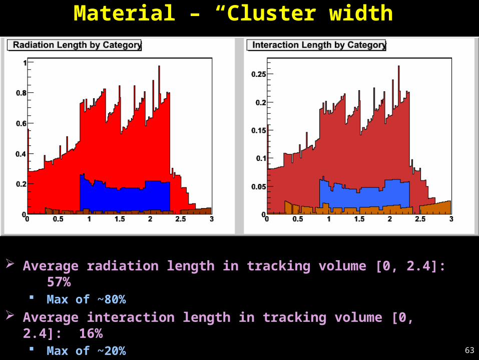
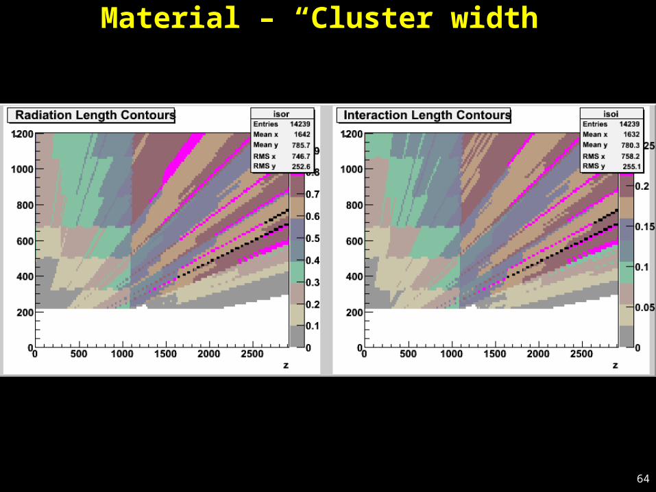
Material – “Cluster width”
Average radiation length in tracking volume [0, 2.4]: 57%
Max of ~80% Average interaction length in tracking volume [0, 2.4]:
16% Max of ~20%
64
Material – “Cluster width”
65
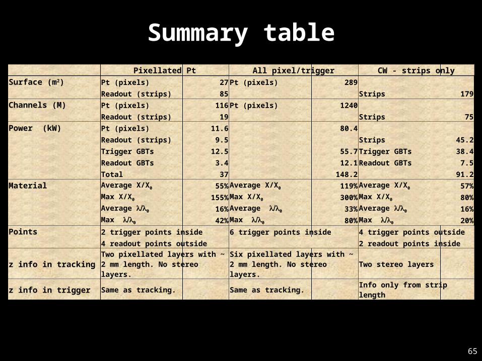
Summary table Pixellated Pt All pixel/trigger CW - strips onlySurface (m2) Pt (pixels) 27Pt (pixels) 289 Readout (strips) 85 Strips 179Channels (M) Pt (pixels) 116Pt (pixels) 1240 Readout (strips) 19 Strips 75Power (kW) Pt (pixels) 11.6 80.4 Readout (strips) 9.5 Strips 45.2 Trigger GBTs 12.5 55.7Trigger GBTs 38.4 Readout GBTs 3.4 12.1Readout GBTs 7.5 Total 37 148.2 91.2Material Average X/X0 55%Average X/X0 119%Average X/X0 57% Max X/X0 155%Max X/X0 300%Max X/X0 80% Average /l l0 16%Average /l l0 33%Average /l l0 16% Max /l l0 42%Max /l l0 80%Max /l l0 20%Points 2 trigger points inside 6 trigger points inside 4 trigger points outside 4 readout points outside 2 readout points inside
z info in tracking Two pixellated layers with ~ 2 mm length. No stereo layers.
Six pixellated layers with ~ 2 mm length. No stereo layers.
Two stereo layers
z info in trigger Same as tracking. Same as tracking. Info only from strip length
66
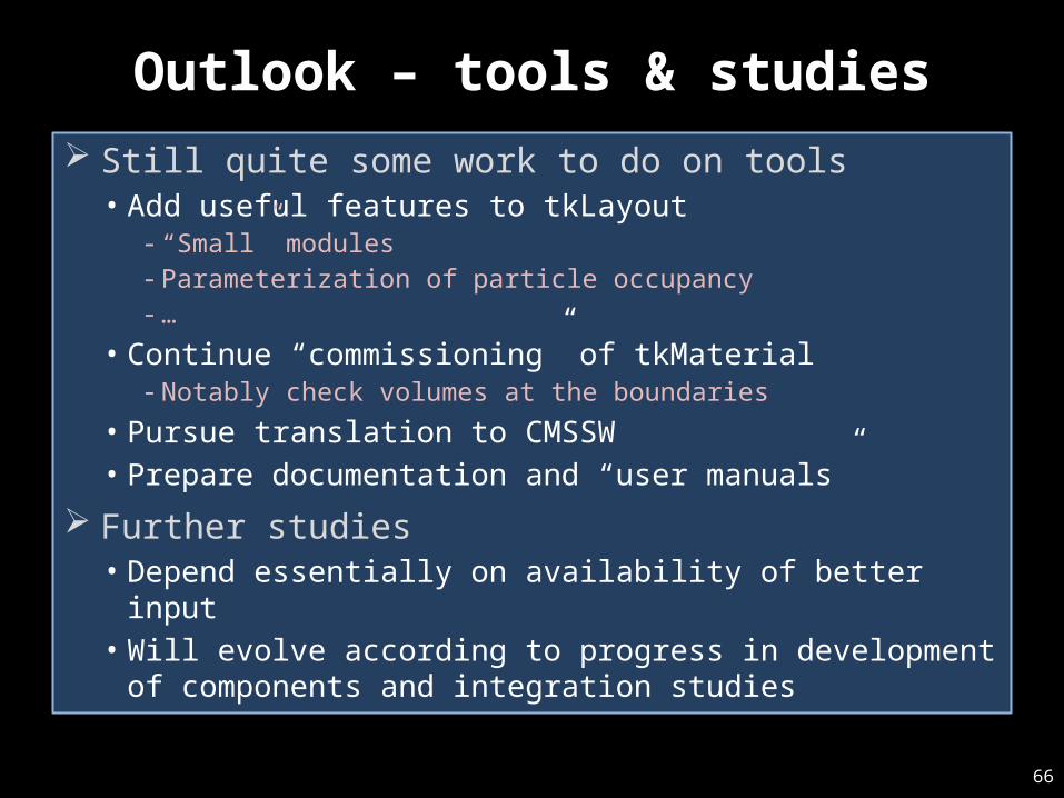
Outlook – tools & studies Still quite some work to do on tools• Add useful features to tkLayout
- “Small” modules- Parameterization of particle occupancy- …
• Continue “commissioning” of tkMaterial- Notably check volumes at the boundaries
• Pursue translation to CMSSW• Prepare documentation and “user manuals”
Further studies• Depend essentially on availability of better input• Will evolve according to progress in development of
components and integration studies
67
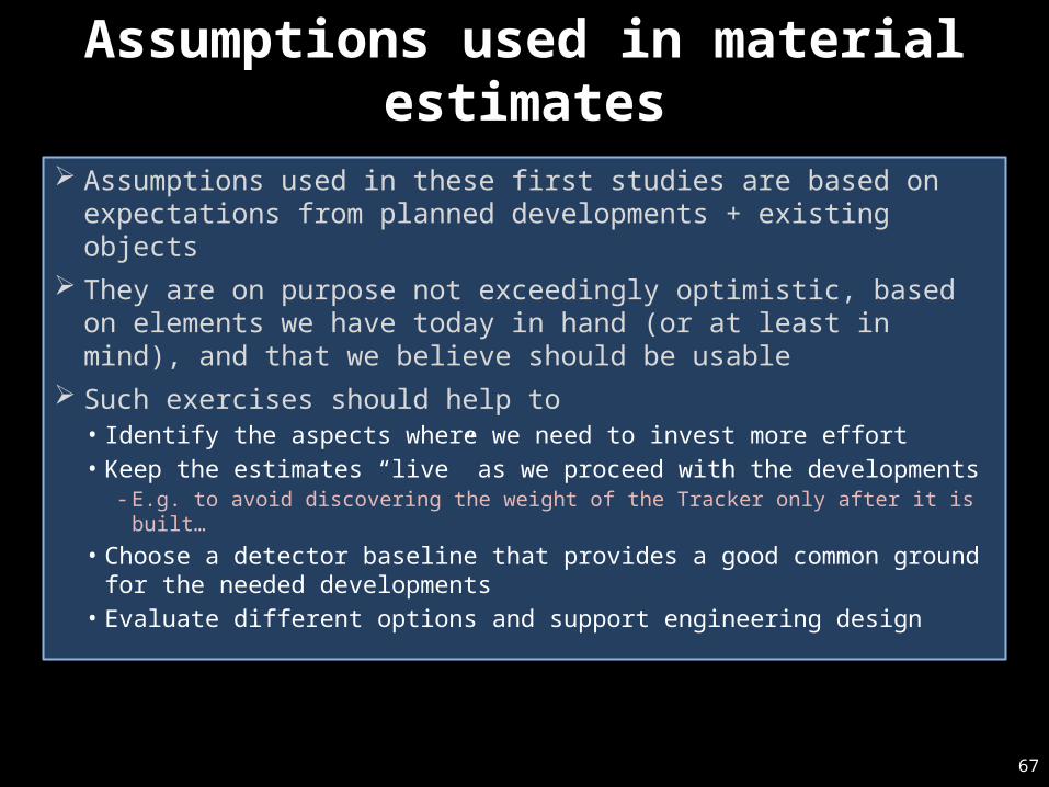
Assumptions used in material estimates
Assumptions used in these first studies are based on expectations from planned developments + existing objects
They are on purpose not exceedingly optimistic, based on elements we have today in hand (or at least in mind), and that we believe should be usable
Such exercises should help to• Identify the aspects where we need to invest more effort• Keep the estimates “live” as we proceed with the developments
- E.g. to avoid discovering the weight of the Tracker only after it is built…
• Choose a detector baseline that provides a good common ground for the needed developments
• Evaluate different options and support engineering design
68
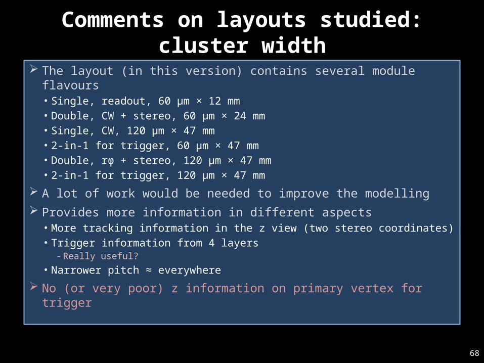
Comments on layouts studied: cluster width
The layout (in this version) contains several module flavours• Single, readout, 60 μm × 12 mm• Double, CW + stereo, 60 μm × 24 mm• Single, CW, 120 μm × 47 mm• 2-in-1 for trigger, 60 μm × 47 mm• Double, rϕ + stereo, 120 μm × 47 mm• 2-in-1 for trigger, 120 μm × 47 mm
A lot of work would be needed to improve the modelling Provides more information in different aspects
• More tracking information in the z view (two stereo coordinates)• Trigger information from 4 layers
- Really useful?
• Narrower pitch ≈ everywhere
No (or very poor) z information on primary vertex for trigger
69
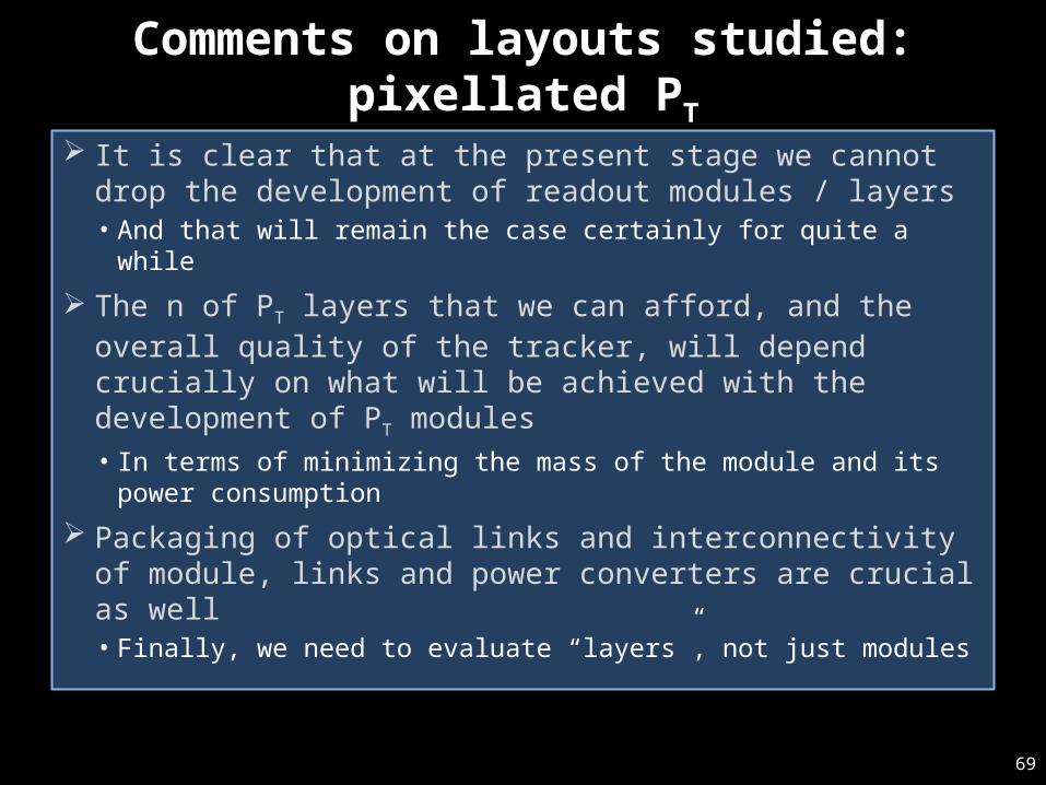
Comments on layouts studied: pixellated PT
It is clear that at the present stage we cannot drop the development of readout modules / layers• And that will remain the case certainly for quite a while
The n of PT layers that we can afford, and the overall quality of the tracker, will depend crucially on what will be achieved with the development of PT modules• In terms of minimizing the mass of the module and its power
consumption
Packaging of optical links and interconnectivity of module, links and power converters are crucial as well• Finally, we need to evaluate “layers”, not just modules

70
Backup
71
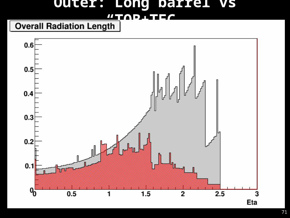
Outer: Long barrel vs “TOB+TEC”
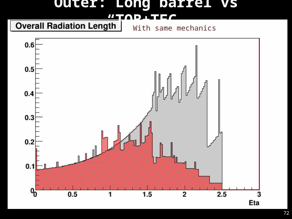
72
Outer: Long barrel vs “TOB+TEC”With same mechanics