Embed Size (px)
Citation preview
lcg
command line electrophysiology
A user manual
Daniele LinaroJoao Couto
Michele Giugliano
6th January 2015

Contents
1 Introduction 11.1 What is LCG? . . . . . . . . . . . . . . . . . . . . . . . . . . . . 1
2 Installation 52.1 Configuration of the Linux box . . . . . . . . . . . . . . . . . . . 5
2.1.1 Patching and installing the real-time kernel . . . . . . . . 52.1.2 Installation of the dependencies . . . . . . . . . . . . . . . 7
2.2 Installation of LCG . . . . . . . . . . . . . . . . . . . . . . . . . . 82.2.1 Installation of the Python bindings . . . . . . . . . . . . . 9
2.3 Final configuration . . . . . . . . . . . . . . . . . . . . . . . . . . 92.4 Installation without a realtime kernel . . . . . . . . . . . . . . . . 112.5 Installing the live medium to a USB drive . . . . . . . . . . . . . 11
2.5.1 From a Debian/Ubuntu distribution . . . . . . . . . . . . 112.5.2 From Windows . . . . . . . . . . . . . . . . . . . . . . . . 12
3 Getting started 133.1 Requirements . . . . . . . . . . . . . . . . . . . . . . . . . . . . . 133.2 First steps in command-line electrophysiology . . . . . . . . . . . 14
3.2.1 Creating an experiment folder . . . . . . . . . . . . . . . . 143.2.2 Recording from a simulated neuron . . . . . . . . . . . . . 143.2.3 Loading files and analyzing data . . . . . . . . . . . . . . 153.2.4 Interfacing with a Patch Clamp amplifier . . . . . . . . . 193.2.5 Your first recording . . . . . . . . . . . . . . . . . . . . . 21
4 Electrophysiology protocols 234.1 Action potential protocol . . . . . . . . . . . . . . . . . . . . . . 234.2 V-I curve protocol . . . . . . . . . . . . . . . . . . . . . . . . . . 244.3 Time constant protocol . . . . . . . . . . . . . . . . . . . . . . . 244.4 Current ramp protocol . . . . . . . . . . . . . . . . . . . . . . . . 244.5 White noise protocol . . . . . . . . . . . . . . . . . . . . . . . . . 254.6 Filtered noise protocol . . . . . . . . . . . . . . . . . . . . . . . . 254.7 Input resistance . . . . . . . . . . . . . . . . . . . . . . . . . . . . 254.8 DC steps protocol . . . . . . . . . . . . . . . . . . . . . . . . . . 264.9 f-I curve protocol . . . . . . . . . . . . . . . . . . . . . . . . . . . 264.10 Frequency clamp protocol . . . . . . . . . . . . . . . . . . . . . . 274.11 Spontaneous activity protocol . . . . . . . . . . . . . . . . . . . . 274.12 Train of pulses protocol . . . . . . . . . . . . . . . . . . . . . . . 274.13 Utility programs . . . . . . . . . . . . . . . . . . . . . . . . . . . 28
i

ii CONTENTS
5 Stimulus generator 295.1 Stimulation files . . . . . . . . . . . . . . . . . . . . . . . . . . . 305.2 Generating stimulation files . . . . . . . . . . . . . . . . . . . . . 31
5.2.1 Examples . . . . . . . . . . . . . . . . . . . . . . . . . . . 32
6 Data files 35
7 Configuration files 377.1 Introduction . . . . . . . . . . . . . . . . . . . . . . . . . . . . . . 37
8 Entities 398.1 H5Recorder . . . . . . . . . . . . . . . . . . . . . . . . . . . . . . 408.2 TriggeredH5Recorder . . . . . . . . . . . . . . . . . . . . . . . . . 408.3 Waveform . . . . . . . . . . . . . . . . . . . . . . . . . . . . . . . 408.4 Constant . . . . . . . . . . . . . . . . . . . . . . . . . . . . . . . 418.5 ConstantFromFile . . . . . . . . . . . . . . . . . . . . . . . . . . 418.6 AnalogInput . . . . . . . . . . . . . . . . . . . . . . . . . . . . . . 418.7 AnalogOutput . . . . . . . . . . . . . . . . . . . . . . . . . . . . . 428.8 AnalogIO . . . . . . . . . . . . . . . . . . . . . . . . . . . . . . . 438.9 RealNeuron . . . . . . . . . . . . . . . . . . . . . . . . . . . . . . 438.10 LIFNeuron . . . . . . . . . . . . . . . . . . . . . . . . . . . . . . 448.11 IzhikevichNeuron . . . . . . . . . . . . . . . . . . . . . . . . . . . 458.12 FrequencyEstimator . . . . . . . . . . . . . . . . . . . . . . . . . 458.13 PID . . . . . . . . . . . . . . . . . . . . . . . . . . . . . . . . . . 468.14 EventCounter . . . . . . . . . . . . . . . . . . . . . . . . . . . . . 468.15 Poisson . . . . . . . . . . . . . . . . . . . . . . . . . . . . . . . . 478.16 Connection . . . . . . . . . . . . . . . . . . . . . . . . . . . . . . 478.17 VariableDelayConnection . . . . . . . . . . . . . . . . . . . . . . 488.18 SynapticConnection . . . . . . . . . . . . . . . . . . . . . . . . . 488.19 PhasicDelay . . . . . . . . . . . . . . . . . . . . . . . . . . . . . . 488.20 SobolDelay . . . . . . . . . . . . . . . . . . . . . . . . . . . . . . 488.21 RandomDelay . . . . . . . . . . . . . . . . . . . . . . . . . . . . . 498.22 PeriodicPulse . . . . . . . . . . . . . . . . . . . . . . . . . . . . . 498.23 PeriodicTrigger . . . . . . . . . . . . . . . . . . . . . . . . . . . . 508.24 ExponentialSynapse . . . . . . . . . . . . . . . . . . . . . . . . . 508.25 Exp2Synapse . . . . . . . . . . . . . . . . . . . . . . . . . . . . . 508.26 TMGSynapse . . . . . . . . . . . . . . . . . . . . . . . . . . . . . 518.27 ConductanceStimulus . . . . . . . . . . . . . . . . . . . . . . . . 518.28 NMDAConductanceStimulus . . . . . . . . . . . . . . . . . . . . 528.29 OU . . . . . . . . . . . . . . . . . . . . . . . . . . . . . . . . . . . 528.30 OUNonStationary . . . . . . . . . . . . . . . . . . . . . . . . . . 528.31 HHSodium . . . . . . . . . . . . . . . . . . . . . . . . . . . . . . 538.32 HHPotassium . . . . . . . . . . . . . . . . . . . . . . . . . . . . . 538.33 HHSodiumCN . . . . . . . . . . . . . . . . . . . . . . . . . . . . . 548.34 HHPotassiumCN . . . . . . . . . . . . . . . . . . . . . . . . . . . 548.35 HH2Sodium . . . . . . . . . . . . . . . . . . . . . . . . . . . . . . 548.36 HH2Potassium . . . . . . . . . . . . . . . . . . . . . . . . . . . . 558.37 MCurrent . . . . . . . . . . . . . . . . . . . . . . . . . . . . . . . 558.38 WBSodium . . . . . . . . . . . . . . . . . . . . . . . . . . . . . . 558.39 WBPotassium . . . . . . . . . . . . . . . . . . . . . . . . . . . . . 56

CONTENTS iii
9 Additional features 579.1 Computation of the SHA checksum . . . . . . . . . . . . . . . . . 579.2 Adding comments to data files . . . . . . . . . . . . . . . . . . . 57
A MATLAB reference 63
B UNIX reference 65

Chapter 1
Introduction
This manual describes the functionalities of lcg, a suite of programs – calledcommands – that can be used to perform electrophysiological experiments.lcg was developed by Daniele Linaro and Joao Couto while at the TheoreticalNeurobiology and Neuroengineering Laboratory of the University of Antwerp.Michele Giugliano developed the concept and meta-description of stimulus filesand implemented the first version of the related source code.
The main features of lcg are the following:
• dynamic clamp capabilities, with built-in active electrode compensationBrette et al. (2008);
• straightforward design and implementation of closed loop and hybrid ex-periments;
• command-line operability;
• ease of automation by scripting;
• compact description of stimulation waveforms;
• simple implementation of non real time protocols (e.g., current and voltageclamp);
• support for multiple real time engines;
• simple installation and operation procedures.
1.1 What is LCG?
lcg is a software toolbox that can be used to perform electrophysiological ex-periments using simple stimulation protocols but also more complex paradigmssuch as dynamic clamp and/or hybrid networks. lcg is made up of two parts:the first one is a C++ library that implements the low-level objects responsible,among other things, of analog input/output, saving data to disk and inter-facing with the real-time scheduling system of the OS. The second part is a
1

2 CHAPTER 1. INTRODUCTION
Python interface that handles simpler tasks, mostly related to the high-leveldescription of specific electrophysiological protocols and simple data analysisand plotting.
lcg consists of a set of commands, each of which performs a specific task.The entry point of all lcg commands is the program called lcg. Its purposeis merely to parse its arguments and call the appropriate protocol with thearguments with which it was invoked. To clarify this concept, let’s look at thefollowing example:
‘‘‘‘ ‘‘1 lcg steps -a -200,100,50 -d 2
This command instructs lcg to look for a program called lcg-steps in thedirectories where executable files are located,1 and invoke it with the subsequentarguments unchanged. The previous call is therefore equivalent to
‘‘‘‘ ‘‘1 lcg -steps -a -200,100,50 -d 2
This approach is particularly suited to adding extensions to lcg: to do so, itis sufficient to follow the naming scheme just described and place additionalscripts or programs where lcg can find them, i.e., anywhere in the path.
lcg comes with a help command, that can be used to display general infor-mation about lcg and a list of the most commonly used protocols, by simplyinvoking
‘‘‘‘ ‘‘1 lcg help
Alternatively, lcg-help accepts one single argument, which must be the nameof a recognized command and invokes it with the -h option. For example, thefollowing four commands produce the same result:
‘‘‘‘ ‘‘1 lcg help steps
‘‘‘‘ ‘‘2 lcg -help steps
‘‘‘‘ ‘‘3 lcg steps -h
‘‘‘‘ ‘‘4 lcg -steps -h
For this to work, all commands must accept the -h option and interpret it as arequest for help. All commands that come with lcg adhere to this convention,and additional ones should do the same.
This manual is organized as follows: Chap. 2 covers in detail the installationof a real-time operating system and of lcg and its dependencies. Chapter 3explains how to start using lcg. Chapter 4 describes the most commonly usedcommands that come with lcg and the related electrophysiological protocols,while Chap. 5 explains how stimulus files can be used to apply arbitrary stimula-tion protocols, in traditional voltage and current clamp experiments. Chapter 6covers the internal organization of the data files saved by lcg and contains a fewexamples that show how to load lcg data files using both Matlab and Python.Chapters 7 through 8 explain how configuration files can be used to describecustom experimental protocols, and which basic building blocks – called enti-ties or streams – are available in lcg. Finally, Chap. 9 covers some additionalfeatures of lcg.
1These are usually stored in the $PATH environment variable.

1.1. WHAT IS LCG? 3
In the simplest scenario, in which lcg is already installed on a machine andthe experimentalist only wants to perform conventional voltage and/or currentclamp experiments, without the need for real time control over the experiment,Chapters 3, 4 and 5 with some parts of Chap. 6 are sufficient to get going.

4 CHAPTER 1. INTRODUCTION

Chapter 2
Installation
The primary application of lcg is to perform electrophysiology experiments.Albeit not necessary, as it will be described in the following, it is howeverrecommended to install lcg on a Linux machine with a data acquisition cardand a working installation of the Comedi library. A real-time kernel is requiredonly to perform closed-loop or dynamic clamp experiments.
It is also possible to install lcg on any UNIX compatible operating system(Linux or Mac OS X, for instance) without Comedi and real-time capabilities.This approach can be useful to familiarize with the program and to develop newexperiments. A detailed description of how to do this is given in Sec. 2.4.
In the following section, we describe how to set up a Linux machine with a real-time kernel and Comedi and how to install lcg. We assume that you have aworking Linux installation: if that is not the case, refer to the documentation ofone of the multiple distributions available. In our laboratory we use Debian andtherefore the following instructions will be based on this distribution.
2.1 Configuration of the Linux box
lcg can be installed on a variety of Linux distributions. Here, we will refer tothe stable version of Debian at the time of this writing (Squeeze 6.0 ).
2.1.1 Patching and installing the real-time kernel
If you don’t want to use the real-time capabilities of lcg you can skip thisparagraph.
This is potentially the most difficult part of the installation. In order to achievenanosecond precision, lcg requires a kernel with real-time capabilities. BothRTAI or PREEMPT RT can be used. The latter is advisable since RTAIdoes not include support for the latest kernels, which might work better withthe most recent hardware.
5

6 CHAPTER 2. INSTALLATION
You may need to install tools to build the kernel. In Debian you can type, asroot:
‘‘‘‘ ‘‘1 apt -get update
‘‘‘‘ ‘‘2 apt -get install build -essential binutils -dev libelf -dev libncurses5
‘‘‘‘ ‘‘libncurses5 -dev git -core make gcc subversion libc6 libc6 -dev
‘‘‘‘ ‘‘automake libtool bison flex autoconf libgsl0 -dev
1. Check which kernels and patches are available. It is advisable toinstall the real-time patch on a “vanilla” kernel. To do so, browse thekernel.org “rt” project page and find out which patches are available forthe kernel that you wish to install. In the following, we will describe howto patch and compile the 3.8.4 version of the Linux kernel.
2. Download the kernel and the real-time patch The directory /us-r/src is a common place to install the Linux kernel. You will need to haveroot privileges to perform these operations.
‘‘‘‘ ‘‘1 cd /usr/src
‘‘‘‘ ‘‘2 wget https :// www.kernel.org/pub/linux/kernel/v3.x/linux -3.8.4.
‘‘‘‘ ‘‘tar.bz2
‘‘‘‘ ‘‘3 wget http :// www.kernel.org/pub/linux/kernel/projects/rt /3.8/
‘‘‘‘ ‘‘patch -3.8.4 - rt2.patch.bz2
3. Decompress and patch the kernel. Patching the kernel will add real-time support to the kernel you have downloaded.
‘‘‘‘ ‘‘1 tar xjf linux -3.8.4. tar.bz2
‘‘‘‘ ‘‘2 ln -s linux -3.8.4 linux
‘‘‘‘ ‘‘3 cd linux
‘‘‘‘ ‘‘4 bzcat ../patch -3.8.4 - rt2.patch.bz2 | patch -p1
4. Configure the kernel. The easiest way to do this is to use the config-uration file from a kernel that was previously installed in your system orfrom a similar installation/system.
‘‘‘‘ ‘‘1 cp /boot/config -‘uname -r‘ .config
‘‘‘‘ ‘‘2 make oldconfig
‘‘‘‘ ‘‘3 make menuconfig
This will evoke a user interface to configure the kernel options. You needto set the Preemption model to Fully Preemptible Kernel (RT) in theProcessor type and features. Disable CPU Frequency scaling un-der Power Management and ACPI options and Check for stack overflow
and all options under Tracers (the latter to make the kernel smaller)in Kernel hacking. Additionally you should also disable the Comedi
drivers under the Staging drivers of the Device drivers menu. Savethe configuration and exit.
5. Compile and install the kernel. This step might take from severalminutes to a few hours, depending on the size of the kernel and on thespeed of your machine.
‘‘‘‘ ‘‘1 make && make modules && make modules_install && make install
When the installation is complete you will need to update the boot loader.
2.1. CONFIGURATION OF THE LINUX BOX 7
‘‘‘‘ ‘‘1 cd /boot
‘‘‘‘ ‘‘2 update -initramfs -c -k 3.8.4 -rt2
‘‘‘‘ ‘‘3 update -grub
Check that grub has been updated. You should see an entry with thename of the newly installed kernel in /etc/grub/menu.lst. You can nowreboot into your new kernel.
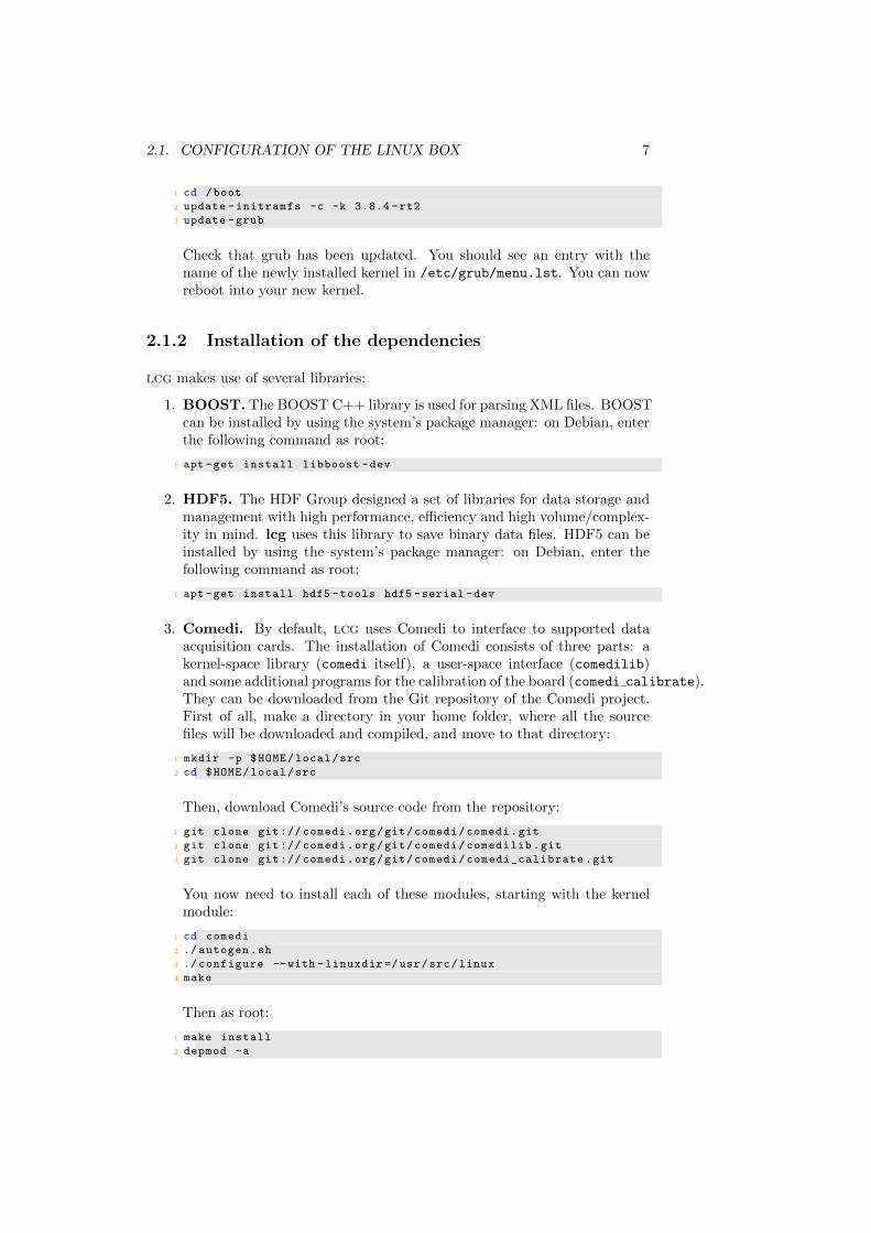
2.1.2 Installation of the dependencies
lcg makes use of several libraries:
1. BOOST. The BOOST C++ library is used for parsing XML files. BOOSTcan be installed by using the system’s package manager: on Debian, enterthe following command as root:
‘‘‘‘ ‘‘1 apt -get install libboost -dev
2. HDF5. The HDF Group designed a set of libraries for data storage andmanagement with high performance, efficiency and high volume/complex-ity in mind. lcg uses this library to save binary data files. HDF5 can beinstalled by using the system’s package manager: on Debian, enter thefollowing command as root:
‘‘‘‘ ‘‘1 apt -get install hdf5 -tools hdf5 -serial -dev
3. Comedi. By default, lcg uses Comedi to interface to supported dataacquisition cards. The installation of Comedi consists of three parts: akernel-space library (comedi itself), a user-space interface (comedilib)and some additional programs for the calibration of the board (comedi calibrate).They can be downloaded from the Git repository of the Comedi project.First of all, make a directory in your home folder, where all the sourcefiles will be downloaded and compiled, and move to that directory:
‘‘‘‘ ‘‘1 mkdir -p $HOME/local/src‘‘‘‘ ‘‘2 cd $HOME/local/src
Then, download Comedi’s source code from the repository:
‘‘‘‘ ‘‘1 git clone git:// comedi.org/git/comedi/comedi.git
‘‘‘‘ ‘‘2 git clone git:// comedi.org/git/comedi/comedilib.git
‘‘‘‘ ‘‘3 git clone git:// comedi.org/git/comedi/comedi_calibrate.git
You now need to install each of these modules, starting with the kernelmodule:
‘‘‘‘ ‘‘1 cd comedi
‘‘‘‘ ‘‘2 ./ autogen.sh
‘‘‘‘ ‘‘3 ./ configure --with -linuxdir =/usr/src/linux
‘‘‘‘ ‘‘4 make
Then as root:
‘‘‘‘ ‘‘1 make install
‘‘‘‘ ‘‘2 depmod -a
8 CHAPTER 2. INSTALLATION
Now for comedilib, the user space interface to the kernel module (run make
install as root):
‘‘‘‘ ‘‘1 cd comedilib
‘‘‘‘ ‘‘2 ./ autogen.sh
‘‘‘‘ ‘‘3 ./ configure --prefix =/usr/local
‘‘‘‘ ‘‘4 make
‘‘‘‘ ‘‘5 make install
And similarly for comedi calibrate, the tools to calibrate the DAQ cards(install the Boost headers before this step):
‘‘‘‘ ‘‘1 cd comedi_calibrate
‘‘‘‘ ‘‘2 ./ autogen.sh
‘‘‘‘ ‘‘3 ./ configure --prefix =/usr/local
‘‘‘‘ ‘‘4 make
‘‘‘‘ ‘‘5 make install
Now that the drivers are installed you need to create the rules to allowusers to access the devices. To do that, create, as root, a file called /
etc/udev/rules.d/99-comedi.rules and add the following line to it:KERNEL=="comedi0", MODE="0666". In case you have multiple acquisi-tion cards, add a line for each of them.
2.2 Installation of LCG
To install lcg, start by getting it from the GitHub repository. We recommendinstalling lcg in a local folder, so that it is easier to have multiple installationsfor different users.
‘‘‘‘ ‘‘1 cd $HOME/local/src‘‘‘‘ ‘‘2 git clone https :// github.com/danielelinaro/dynclamp.git lcg
‘‘‘‘ ‘‘3 cd lcg
‘‘‘‘ ‘‘4 autoreconf -i
‘‘‘‘ ‘‘5 ./ configure --prefix=$HOME/local‘‘‘‘ ‘‘6 make
‘‘‘‘ ‘‘7 make install
If you are installing lcg on a real-time machine, you need to create a realtimegroup to allow non-root users to run lcg commands. To do so, as root add thefollowing lines to /etc/security/limits.conf.
‘‘‘‘ ‘‘1 @realtime - rtprio 99
‘‘‘‘ ‘‘2 @realtime - memlock unlimited
Then, create a group realtime and add the users that you want to be able touse lcg.
‘‘‘‘ ‘‘1 groupadd realtime
‘‘‘‘ ‘‘2 usermod -a -G realtime USER
where USER is the actual login name of an existing user. You need to log outand log back in for the changes to take effect.

2.3. FINAL CONFIGURATION 9
2.2.1 Installation of the Python bindings
lcg comes with a set of Python scripts that can be used both to performstandard electrophysiology experiments and as starting point for developingnew protocols.
The full list of available protocols (called commands, in lcg terminology) is de-scribed in Chapter 4: here, we only describe how to install the Python bindingsand their dependencies.
Start by installing numpy, scipy, matplotlib and pytables if they are notalready present on your system. In Debian this can be accomplished with thefollowing command:
‘‘‘‘ ‘‘1 apt -get install python -setuptools python -numpy python -scipy python -
‘‘‘‘ ‘‘matplotlib python -tables python -lxml
Alternatively, to have the latest version of the modules, you can install themfrom source.
To install lcg Python modules, from the base directory (i.e., where you clonedthe Git repository) type:
‘‘‘‘ ‘‘1 export PYTHONPATH=$PYTHONPATH:$HOME/local/lib/python2 .7/site -‘‘‘‘ ‘‘packages
‘‘‘‘ ‘‘2 cd python
‘‘‘‘ ‘‘3 python setup.py build
‘‘‘‘ ‘‘4 python setup.py install --prefix=$HOME/local
In case you are using a different version of Python (2.6, for instance), change thedirectory accordingly (i.e., to $HOME/local/lib/python2.6/site-packages).
This will install the module in the directory $HOME/local/lib/python2.7/site-packages, which needs to be permanently added to your PYTHONPATH
environment variable, by adding the previous export line to your .bashrc file.This can be accomplished with the following command:
‘‘‘‘ ‘‘1 echo ’export PYTHONPATH=$PYTHONPATH:$HOME/local/lib/python2 .7/site -‘‘‘‘ ‘‘packages ’ >> $HOME/. bashrc
Again, change the directory accordingly if you are using a different Pythonversion. You can test whether the installation was successful by issuing thefollowing commands:
‘‘‘‘ ‘‘1 cd $HOME‘‘‘‘ ‘‘2 python
‘‘‘‘ ‘‘3 import lcg
If the last command produces no error, the installation was successfull.
2.3 Final configuration
In order for lcg to function properly, a few configuration steps must be com-pleted. First of all, add the directory where lcg binaries were installed to yourpath. To do this, add the following line to your .bashrc file:
10 CHAPTER 2. INSTALLATION
‘‘‘‘ ‘‘1 export PATH=$PATH:$HOME/local/bin
After this, copy the files lcg-env.sh and lcg-completion.bash from lcg basedirectory to your home directory:
‘‘‘‘ ‘‘1 cp lcg -env.sh ~/.lcg -env.sh
‘‘‘‘ ‘‘2 cp lcg -completion.bash ~/.lcg -completion.bash
Source them any time you log in by adding the following lines to your .bashrcfile:
‘‘‘‘ ‘‘1 source ~/.lcg -env.sh
‘‘‘‘ ‘‘2 source ~/.lcg -completion.bash
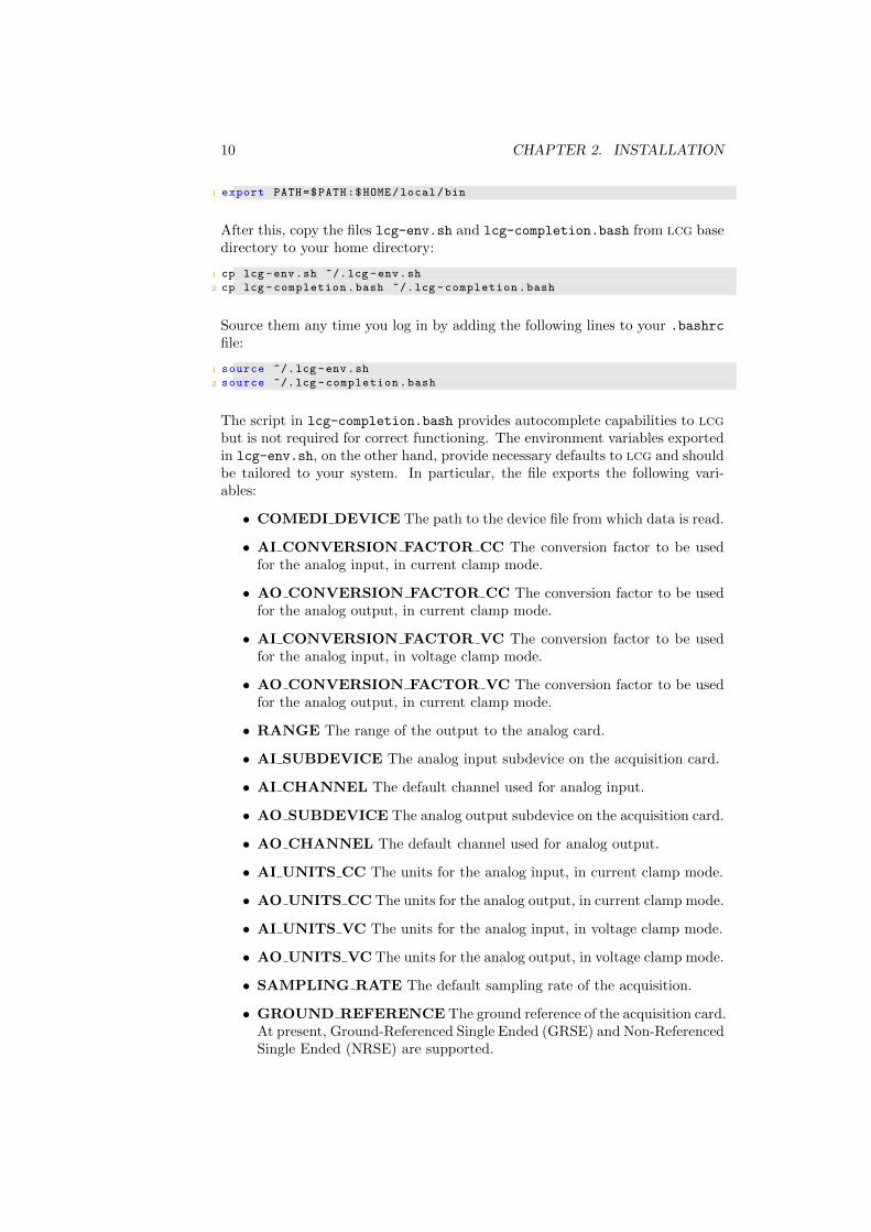
The script in lcg-completion.bash provides autocomplete capabilities to lcgbut is not required for correct functioning. The environment variables exportedin lcg-env.sh, on the other hand, provide necessary defaults to lcg and shouldbe tailored to your system. In particular, the file exports the following vari-ables:
• COMEDI DEVICE The path to the device file from which data is read.
• AI CONVERSION FACTOR CC The conversion factor to be usedfor the analog input, in current clamp mode.
• AO CONVERSION FACTOR CC The conversion factor to be usedfor the analog output, in current clamp mode.
• AI CONVERSION FACTOR VC The conversion factor to be usedfor the analog input, in voltage clamp mode.
• AO CONVERSION FACTOR VC The conversion factor to be usedfor the analog output, in current clamp mode.
• RANGE The range of the output to the analog card.
• AI SUBDEVICE The analog input subdevice on the acquisition card.
• AI CHANNEL The default channel used for analog input.
• AO SUBDEVICE The analog output subdevice on the acquisition card.
• AO CHANNEL The default channel used for analog output.
• AI UNITS CC The units for the analog input, in current clamp mode.
• AO UNITS CC The units for the analog output, in current clamp mode.
• AI UNITS VC The units for the analog input, in voltage clamp mode.
• AO UNITS VC The units for the analog output, in voltage clamp mode.
• SAMPLING RATE The default sampling rate of the acquisition.
• GROUND REFERENCE The ground reference of the acquisition card.At present, Ground-Referenced Single Ended (GRSE) and Non-ReferencedSingle Ended (NRSE) are supported.

2.4. INSTALLATION WITHOUT A REALTIME KERNEL 11
• LCG REALTIME This variable tells whether the system should prefer-entially use the real-time kernel if it is available or not. The main advan-tage in using the real-time kernel (also for open loop experiments) is thatit provides synchronous input and output, in contrast to the non-real-timemode, where input and output are asynchronously managed by the DAQboard.
• LCG RESET OUTPUT This variable tells whether the output of theDAQ board should automatically be reset to zero every time a trial ends.This is particularly useful when interrupting the program (with Ctrl-C forexample) and is valid only for current clamp experiments.
Most of the previous values depend on how your amplifier is configured and onhow it is wired to the acquisition card. It is also important to note that theconversion factors and the units provided in .lcg-env.sh are meaningful whenonly one input and output channel are present. In all other cases, input/outputconversion factors will have to be specified either in the configuration file orwhen invoking a script. lcg provides a script that helps the user in finding thecorrect values for the conversion factors used on his/her system. To use it, turnon the amplifier and connect it to the board as you would during an experimentand run the following commands:
‘‘‘‘ ‘‘1 $ comedi_calibrate
‘‘‘‘ ‘‘2 $ lcg -find -conversion -factors --CC-channels 0,0 --VC-channels 1,1
where the --CC-channels and --VC-channels options specify the input andoutput channels to use in current or voltage clamp mode, respectively, andshould reflect the values used in the system that is being configured. The scriptwill ask the user a few questions and then update the values of the conversionfactors in the .lcg-env.sh file: due to rounding errors, however, these valuesmight have to be rounded by the user afterwards by editing manually the .lcg
-env.sh file.
2.4 Installation without a realtime kernel
If you want to learn how to work with lcg or test configuration files, it ispossible to install lcg on your personal computer. lcg can be compiled onany UNIX-like operating system, such as Linux and Mac OS X. To do so, youjust need to install BOOST and the HDF5 library (see Sec. 2.1.2). The procedureto install lcg is the same as described in Sec. 2.2: the configure script willdetect the absence of Comedi and of the real-time kernel and not compile partsof lcg. If you are installing lcg on Mac OS X, note that the equivalent of the.bashrc file is called .profile.
2.5 Installing the live medium to a USB drive
2.5.1 From a Debian/Ubuntu distribution
This can be done from the command-line:

12 CHAPTER 2. INSTALLATION
2.5.2 From Windows
In order to make a bootable LCG USB drive you can use UNetBootin.

Chapter 3
Getting started
This chapter will help you understanding some basic concepts related to lcg.It starts by giving a notion of the basic commands using an artificial neuronand continues to interfacing with live cells. While it does not intend to be adetailed tutorial on either Matlab or Oython, some indications on how to usethese software packages will be provided.
3.1 Requirements
In order to get started you only need to boot your computer using the live DVDavailable at http://www.tnb.ua.ac.be/LCGliveCD.iso. Instructions aboutsetting up a live USB medium are available in section 2.5. Although all exper-iments can be performed from the live medium, for production environmentsit is better to have a dedicated installation of lcg. Additional notes on theinstallation can be found in section 2.
If you are using a system that someone else installed you can check wether lcgis installed by typing which lcg in a terminal window: if the result is blank,the program has not been installed and you should either use the live DVD orinstall it yourself.
We assume that the reader is somehow familiar with the GNU/Linux operat-ing system and in particular with the usage of a terminal prompt: however,please bear in mind that this is not a Linux tutorial. Check the webpage ofyour GNU/Linux distribution (e.g. Debian; Canonical Ubuntu; Fedora) or thelinux.org tutorials for help on getting started with GNU/Linux. Additionally,the Advanced Bash-Scripting guide from The Linux Documentation Project isa great reference for how to use a UNIX terminal efficiently.
Additionally, some MATLAB and Python code will be used to load data gen-erated with lcg. and therefore working knowledge of either of these languagesis beneficial. Before getting started using lcg you may want to take a look atAppendix A for a short Matlab introduction and Appendix B for some notes onbasic UNIX commands.
13

14 CHAPTER 3. GETTING STARTED
3.2 First steps in command-line electrophysiol-ogy
The most important concepts related to the everyday usage of lcg can be un-derstood by using a neuron model: in this chapter we will use a leaky integrate-and-fire (LIF) model: for an excellent introduction to this and other neuronmodels, see Koch and Segev (1989). The initial part of this guide does notrequire a realtime kernel nor a data acquisiton board. We will illustrate someexamples of usage of lcg as well as some basic concepts of data analysis ofintracellular traces using Python and Octave/Matlab. This should allow a userthat is not familiar with Python nor Matlab® to understand the basics andprovide building blocks for more complete analyses. A good reference for get-ting started with Matlab® is Wallisch (2011) or the resources available on theMathworks. For Python we suggest the Scipy lecture notes. We will also tryto highlight some basic UNIX commands to handle file operations and suggestways to structure and organize your experiments.
3.2.1 Creating an experiment folder
lcg does not require a particular folder structure to be used: when you run acommand the recording will be executed in that very same directory. It is how-ever beneficial to use a consistent folder structure. You can use lcg-create-experiment-folderfor that:
‘‘‘‘ ‘‘lcg -create -experiment -folder -p YYYYMMDD_tutorial_ [001] -s LIFsteps
‘‘‘‘ ‘‘,steps
lcg-create-experiment-folder can do more than creating a folder: amongits features is the capability of adding information files with details about theexperiment.
After running the previous command, the name of the folder that was just cre-ated will be printed to the terminal. Move into this folder using the UNIX com-mand cd <foldername>. By using the command ls you can list the subfold-ers created by lcg-create-experiment-folder, namely LIFsteps and steps.lcg-create-experiment-folder also created a folder 01 inside each of thesewith the intention of storing different sets of trials related to the same proto-col.
3.2.2 Recording from a simulated neuron
As a first example, we will compute the frequency-current (f-I) curve of a LIFmodel neuron. For this we will use the lcg-steps protocol with the --model
option. Run the following commands in the terminal window (what follows #is a comment).
‘‘‘‘ ‘‘# Move into the stepsLIF /01 directory
‘‘‘‘ ‘‘cd LIFsteps /01
‘‘‘‘ ‘‘# Run the protocol
‘‘‘‘ ‘‘lcg -steps -a -200,800,50 -d 1 --model --no -shuffle -n 1
3.2. FIRST STEPS IN COMMAND-LINE ELECTROPHYSIOLOGY 15
‘‘‘‘ ‘‘# Plot the results
‘‘‘‘ ‘‘lcg -plot -f all
Most lcg commands have multiple switches or options that usually have defaultparameters. Make sure that the default parameters fit your purpose, otherwiseuse switches to set them. All protocols have a --help switch that displays thesupported options and default parameters.
In the above example you used lcg to inject DC current steps from −200 to800 pA in 50 pA steps and 1 s duration into a simulated neuron. The --no-shuffleoption tells lcg-steps not to shuffle the current amplitudes.
3.2.3 Loading files and analyzing data
Analyzing the recorded data is arguably on of the most important steps of anexperiment. While this manual does not intend to go into details on the dataanalysis we will show examples of scripts to visualize and analyze data for thissimple case. Before proceeding you should understand the basic structure of thedata files recorded by lcg when using HDF5 files. For a detailed explanationread chapter 6. Each file contains at least 2 groups Entities and Info. TheEntities group contains each element (entity; see 8) of the recording: in thiscase the recorded voltage trace and the injected current step. It should be notedthat each entity can also contain metadata representing its parameters, suchas the stimuli parameters for the Waveform entity. The Info group containsparameters of the experiment such as the time step (dt) used and the duration(tend) of the recording.
Python implementation
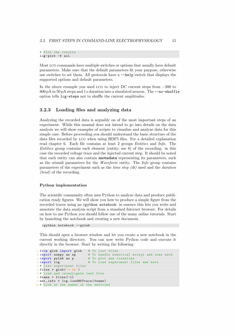
The scientific community often uses Python to analyze data and produce publi-cation ready figures. We will show you how to produce a simple figure from therecorded traces using an ipython notebook: in essence this lets you write andannotate the data analysis script from a standard Internet browser. For detailson how to use Python you should follow one of the many online tutorials. Startby launching the notebook and creating a new document.
‘‘‘‘ ‘‘ipython notebook --pylab
This should open a browser window and let you create a new notebook in thecurrent working directory. You can now write Python code and execute itdirectly in the browser. Start by writing the following:
‘‘‘‘ ‘‘1 from glob import glob # To list files
‘‘‘‘ ‘‘2 import numpy as np # To handle numerical arrays and some math
‘‘‘‘ ‘‘3 import pylab as p # To plot and visualize
‘‘‘‘ ‘‘4 import lcg # To load experiment files and more
‘‘‘‘ ‘‘5 # List experiment files
‘‘‘‘ ‘‘6 files = glob('*.h5')‘‘‘‘ ‘‘7 # Load and investigate last file
‘‘‘‘ ‘‘8 fname = files [-1]
‘‘‘‘ ‘‘9 ent ,info = lcg.loadH5Trace(fname)
‘‘‘‘ ‘‘10 # Look at the names of the entities
16 CHAPTER 3. GETTING STARTED
‘‘‘‘ ‘‘11 print [e['name'] for e in ent]
‘‘‘‘ ‘‘12 # Thus the first entity is the Neuron and second entity the
‘‘‘‘ ‘‘Waveform
‘‘‘‘ ‘‘13
‘‘‘‘ ‘‘14 # Create a time vector
‘‘‘‘ ‘‘15 #(This is done using size of the data and the sampling rate (1/dt))
‘‘‘‘ ‘‘16 time = np.arange(len(ent [0]['data']))*info['dt']‘‘‘‘ ‘‘17 # Plot the data in 2 plots with shared x axis
‘‘‘‘ ‘‘18 fig , ax = p.subplots(len(entities) ,1, sharex=True)
‘‘‘‘ ‘‘19 for i,e in enumerate(ent):
‘‘‘‘ ‘‘20 # Plot the data
‘‘‘‘ ‘‘21 ax[i].plot(time , e['data'])‘‘‘‘ ‘‘22 # Add labels with the information from each entity
‘‘‘‘ ‘‘23 ax[i]. set_xlabel('Time (s)')‘‘‘‘ ‘‘24 ystr = '{0} entity ({1}) '.format(e['name'],e['units '])‘‘‘‘ ‘‘25 ax[i]. set_ylabel(ystr)
‘‘‘‘ ‘‘26 # Set the filename as title
‘‘‘‘ ‘‘27 ax[0]. set_title('Data from file {0}'.format(fname))
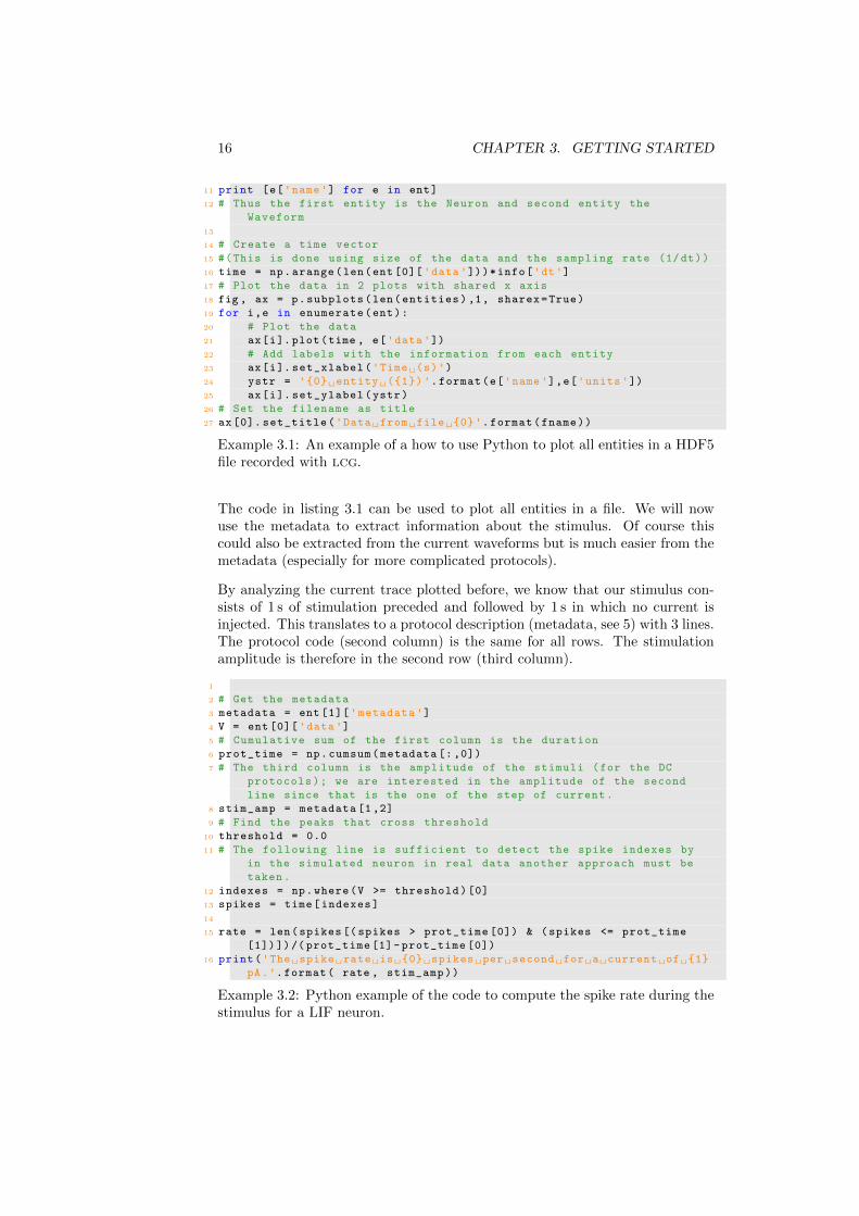
Example 3.1: An example of a how to use Python to plot all entities in a HDF5file recorded with lcg.
The code in listing 3.1 can be used to plot all entities in a file. We will nowuse the metadata to extract information about the stimulus. Of course thiscould also be extracted from the current waveforms but is much easier from themetadata (especially for more complicated protocols).
By analyzing the current trace plotted before, we know that our stimulus con-sists of 1 s of stimulation preceded and followed by 1 s in which no current isinjected. This translates to a protocol description (metadata, see 5) with 3 lines.The protocol code (second column) is the same for all rows. The stimulationamplitude is therefore in the second row (third column).
‘‘‘‘ ‘‘1
‘‘‘‘ ‘‘2 # Get the metadata
‘‘‘‘ ‘‘3 metadata = ent [1]['metadata ']‘‘‘‘ ‘‘4 V = ent [0]['data']‘‘‘‘ ‘‘5 # Cumulative sum of the first column is the duration
‘‘‘‘ ‘‘6 prot_time = np.cumsum(metadata [:,0])
‘‘‘‘ ‘‘7 # The third column is the amplitude of the stimuli (for the DC
‘‘‘‘ ‘‘protocols); we are interested in the amplitude of the second
‘‘‘‘ ‘‘line since that is the one of the step of current.
‘‘‘‘ ‘‘8 stim_amp = metadata [1,2]
‘‘‘‘ ‘‘9 # Find the peaks that cross threshold
‘‘‘‘ ‘‘10 threshold = 0.0
‘‘‘‘ ‘‘11 # The following line is sufficient to detect the spike indexes by
‘‘‘‘ ‘‘in the simulated neuron in real data another approach must be
‘‘‘‘ ‘‘taken.
‘‘‘‘ ‘‘12 indexes = np.where(V >= threshold)[0]
‘‘‘‘ ‘‘13 spikes = time[indexes]
‘‘‘‘ ‘‘14
‘‘‘‘ ‘‘15 rate = len(spikes [( spikes > prot_time [0]) & (spikes <= prot_time
‘‘‘‘ ‘‘[1])])/( prot_time [1]- prot_time [0])
‘‘‘‘ ‘‘16 print('The spike rate is {0} spikes per second for a current of {1}‘‘‘‘ ‘‘pA.'.format( rate , stim_amp))
Example 3.2: Python example of the code to compute the spike rate during thestimulus for a LIF neuron.
3.2. FIRST STEPS IN COMMAND-LINE ELECTROPHYSIOLOGY 17
The spike rate is then simply the number of spikes emitted during the applicationof the current step divided by its duration (1 s in this case). We can now iteratethrough all the files and compute the f-I curve, i.e., the spike rate versus theinjected current.
‘‘‘‘ ‘‘1 def computeRateForLIF(time , V, metadata , threshold =0.0):
‘‘‘‘ ‘‘2 # Function to compute the rate and return the stimulus
‘‘‘‘ ‘‘amplitude
‘‘‘‘ ‘‘3 # for a LIF neuron. See previous python code example.
‘‘‘‘ ‘‘4 prot_time = np.cumsum(metadata [:,0])
‘‘‘‘ ‘‘5 stim_amp = metadata [1,2]
‘‘‘‘ ‘‘6 indexes = np.where(V >= threshold)[0]
‘‘‘‘ ‘‘7 spikes = time[indexes]
‘‘‘‘ ‘‘8 rate = len(spikes [( spikes > prot_time [0]) & (spikes <=
‘‘‘‘ ‘‘prot_time [1])])/( prot_time [1]- prot_time [0])
‘‘‘‘ ‘‘9 return rate , stim_amp
‘‘‘‘ ‘‘10
‘‘‘‘ ‘‘11 # List experiment files
‘‘‘‘ ‘‘12 files = glob(’*.h5’)
‘‘‘‘ ‘‘13 F = []
‘‘‘‘ ‘‘14 I = []
‘‘‘‘ ‘‘15 # Iterate through the files
‘‘‘‘ ‘‘16 for fname in files:
‘‘‘‘ ‘‘17 ent ,info = lcg.loadH5Trace(fname)
‘‘‘‘ ‘‘18 V = ent [0][’data’]
‘‘‘‘ ‘‘19 metadata = ent [1][’metadata ’]
‘‘‘‘ ‘‘20 time = np.arange(len(V))*info[’dt’]
‘‘‘‘ ‘‘21 # Use our function
‘‘‘‘ ‘‘22 tmp_rate ,tmp_stim = computeRateForLIF(time ,V,metadata)
‘‘‘‘ ‘‘23 F.append(tmp_rate)
‘‘‘‘ ‘‘24 I.append(tmp_stim)
‘‘‘‘ ‘‘25 # Make list an numpy.array to sort it so that plotting locks nicer
‘‘‘‘ ‘‘26 F = np.array(F)
‘‘‘‘ ‘‘27 F = F[np.argsort(I)]
‘‘‘‘ ‘‘28 I = np.sort(I)
‘‘‘‘ ‘‘29 # Plot and add axis labels
‘‘‘‘ ‘‘30 p.plot(I,F,’ko-’, clip_on=False)
‘‘‘‘ ‘‘31 p.xlabel(’Current (pA)’)
‘‘‘‘ ‘‘32 p.ylabel(’Rate (spikes per second)’)
‘‘‘‘ ‘‘33 p.grid(True)
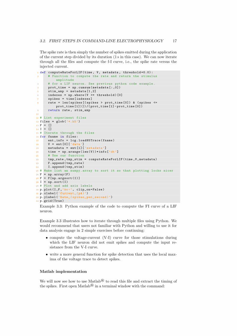
Example 3.3: Python example of the code to compute the FI curve of a LIFneuron.
Example 3.3 illustrates how to iterate through multiple files using Python. Wewould recommend that users not familiar with Python and willing to use it fordata analysis engage in 2 simple exercises before continuing:
• compute the voltage-current (V-I) curve for those stimulations duringwhich the LIF neuron did not emit spikes and compute the input re-sistance from the V-I curve.
• write a more general function for spike detection that uses the local max-ima of the voltage trace to detect spikes.
Matlab implementation
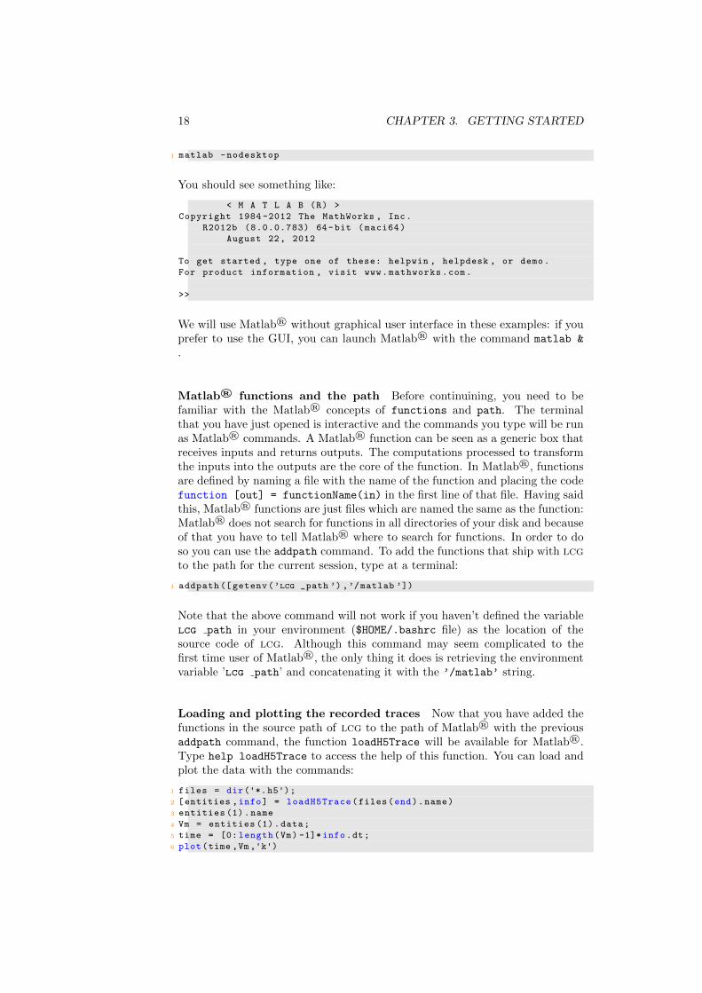
We will now see how to use Matlab® to read this file and extract the timing ofthe spikes. First open Matlab® in a terminal window with the command:
18 CHAPTER 3. GETTING STARTED
‘‘‘‘ ‘‘1 matlab -nodesktop
You should see something like:
‘‘‘‘ ‘‘< M A T L A B (R) >
‘‘‘‘ ‘‘Copyright 1984 -2012 The MathWorks , Inc.
‘‘‘‘ ‘‘R2012b (8.0.0.783) 64-bit (maci64)
‘‘‘‘ ‘‘August 22, 2012
‘‘‘‘ ‘‘
‘‘‘‘ ‘‘To get started , type one of these: helpwin , helpdesk , or demo.
‘‘‘‘ ‘‘For product information , visit www.mathworks.com.
‘‘‘‘ ‘‘
‘‘‘‘ ‘‘>>
We will use Matlab® without graphical user interface in these examples: if youprefer to use the GUI, you can launch Matlab® with the command matlab &
.
Matlab® functions and the path Before continuining, you need to befamiliar with the Matlab® concepts of functions and path. The terminalthat you have just opened is interactive and the commands you type will be runas Matlab® commands. A Matlab® function can be seen as a generic box thatreceives inputs and returns outputs. The computations processed to transformthe inputs into the outputs are the core of the function. In Matlab®, functionsare defined by naming a file with the name of the function and placing the codefunction [out] = functionName(in) in the first line of that file. Having saidthis, Matlab® functions are just files which are named the same as the function:Matlab® does not search for functions in all directories of your disk and becauseof that you have to tell Matlab® where to search for functions. In order to doso you can use the addpath command. To add the functions that ship with lcgto the path for the current session, type at a terminal:
‘‘‘‘ ‘‘1 addpath ([ getenv(’lcg _path ’) ,’/matlab ’])
Note that the above command will not work if you haven’t defined the variablelcg path in your environment ($HOME/.bashrc file) as the location of thesource code of lcg. Although this command may seem complicated to thefirst time user of Matlab®, the only thing it does is retrieving the environmentvariable ’lcg path’ and concatenating it with the ’/matlab’ string.
Loading and plotting the recorded traces Now that you have added thefunctions in the source path of lcg to the path of Matlab® with the previousaddpath command, the function loadH5Trace will be available for Matlab®.Type help loadH5Trace to access the help of this function. You can load andplot the data with the commands:
‘‘‘‘ ‘‘1 files = dir('*.h5');‘‘‘‘ ‘‘2 [entities ,info] = loadH5Trace(files(end).name)
‘‘‘‘ ‘‘3 entities (1).name
‘‘‘‘ ‘‘4 Vm = entities (1).data;
‘‘‘‘ ‘‘5 time = [0: length(Vm) -1]*info.dt;
‘‘‘‘ ‘‘6 plot(time ,Vm ,'k')
3.2. FIRST STEPS IN COMMAND-LINE ELECTROPHYSIOLOGY 19
The first line uses Matlab®’s command dir to list all directories. Then loadH5Trace
loads the data into the variables entities and info - it loads one structure perentity connected to the H5Recorder.The third line in the above code illustrates how you can find out the name ofan entity in the entities array. This can be particularly useful since it letsyou find a particular entity based on its type. Later we will see how to takeadvantage of this feature. The fourth and fifth line we associate the variableVm to the recorded membrane potential of the LIFNeuron and create a timevector with the size of Vm and the time step saved in the info structure.The last line plots the membrane voltage as a function of time using the colorblack.
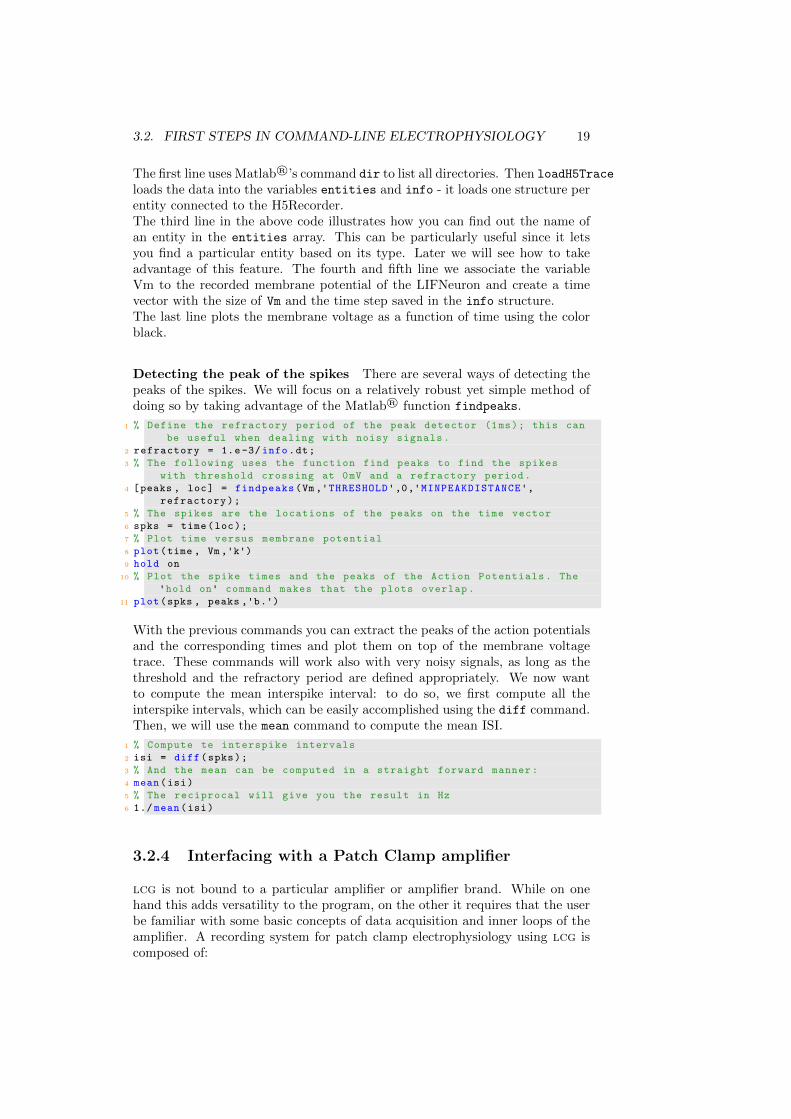
Detecting the peak of the spikes There are several ways of detecting thepeaks of the spikes. We will focus on a relatively robust yet simple method ofdoing so by taking advantage of the Matlab® function findpeaks.
‘‘‘‘ ‘‘1 % Define the refractory period of the peak detector (1ms); this can
‘‘‘‘ ‘‘be useful when dealing with noisy signals.
‘‘‘‘ ‘‘2 refractory = 1.e-3/ info.dt;
‘‘‘‘ ‘‘3 % The following uses the function find peaks to find the spikes
‘‘‘‘ ‘‘with threshold crossing at 0mV and a refractory period.
‘‘‘‘ ‘‘4 [peaks , loc] = findpeaks(Vm ,'THRESHOLD',0,'MINPEAKDISTANCE',‘‘‘‘ ‘‘refractory);
‘‘‘‘ ‘‘5 % The spikes are the locations of the peaks on the time vector
‘‘‘‘ ‘‘6 spks = time(loc);
‘‘‘‘ ‘‘7 % Plot time versus membrane potential
‘‘‘‘ ‘‘8 plot(time , Vm,'k')‘‘‘‘ ‘‘9 hold on
‘‘‘‘ ‘‘10 % Plot the spike times and the peaks of the Action Potentials. The
‘‘‘‘ ‘‘'hold on' command makes that the plots overlap.
‘‘‘‘ ‘‘11 plot(spks , peaks ,'b.')
With the previous commands you can extract the peaks of the action potentialsand the corresponding times and plot them on top of the membrane voltagetrace. These commands will work also with very noisy signals, as long as thethreshold and the refractory period are defined appropriately. We now wantto compute the mean interspike interval: to do so, we first compute all theinterspike intervals, which can be easily accomplished using the diff command.Then, we will use the mean command to compute the mean ISI.
‘‘‘‘ ‘‘1 % Compute te interspike intervals
‘‘‘‘ ‘‘2 isi = diff(spks);
‘‘‘‘ ‘‘3 % And the mean can be computed in a straight forward manner:
‘‘‘‘ ‘‘4 mean(isi)
‘‘‘‘ ‘‘5 % The reciprocal will give you the result in Hz
‘‘‘‘ ‘‘6 1./ mean(isi)
3.2.4 Interfacing with a Patch Clamp amplifier
lcg is not bound to a particular amplifier or amplifier brand. While on onehand this adds versatility to the program, on the other it requires that the userbe familiar with some basic concepts of data acquisition and inner loops of theamplifier. A recording system for patch clamp electrophysiology using lcg iscomposed of:

20 CHAPTER 3. GETTING STARTED
1. a patch-clamp Amplifier.
2. A Data Acquisition Board, referred to as DAQ throughout this manual.
3. A recording computer running lcg.
Assuming that the DAQ board is supported by the COMEDI drivers (or otherdrivers supported by lcg) then it is necessary that the recording computerunderstand what the values being read through the DAQ card mean in termsof the physical quantities being measured. This is accomplished in lcg by a setof environment variables.1 In essence we need to know:
1. where to measure from and what that measure means.
2. Where to stimulate to and how to output something meaningful.
All this information is set up during the installation (see section 2.3) simply byediting a text file.
CC output (Voltage)
VC input (Command Voltage)
CC input (Command Current)
VC output (Current)
Analog InputsAI_CHANNEL
AI_CONVERSION_FACTOR_VC
AI_CONVERSION_FACTOR_CC
Analog OutputsAO_CHANNEL
AO_CONVERSION_FACTOR_VC
AO_CONVERSION_FACTOR_CC
Computer - LCG
Patch Clamp Ampli�er
Figure 3.1: Correspondence between Digital Data Acquisition board and thepatch clamp amplifier.
Figure 3.1 illustrates the most important connections and environment variablesrequired to control the amplifier both in current clamp and in voltage clampmode. Protocols run in current clamp mode use the environment variables withCC suffix while those run in voltage clamp mode use the VC suffix. This allowsdifferent gains, channels and units to be used with minimal interaction from theuser side.
The majority of lcg commands make sense in current clamp mode and there-fore use the corresponding conversion factors. However, those protocols thatcan be used both in voltage and current clamp modes (for instance, the stepsprotocol described before) use by default the current clamp conversion factors,but have an additional –voltage-clamp switch that instructs the command
1If you do not know what a bash environment variable is, please refer to a bash introductorycourse.
3.2. FIRST STEPS IN COMMAND-LINE ELECTROPHYSIOLOGY 21
to use the corresponding conversion factors. A small command called lcg-find-conversion-factors can help quickly discovering the conversion factorsassociated with the patch clamp amplifier.
3.2.5 Your first recording
Once you have configured the environmental variables as described in section2.3, lcg is ready to be used for patch clamp recordings. We can now attemptto characterize the V-I and f-I curves of a real cell as we did for the LIF neuronat the beginning of this chapter. This can be accomplished simply by runningthe lcg-steps protocol.Set the amplifier to current clamp (CC) mode and enable the external command(if required by the patch clamp amplifier). You can now use the Active ElectrodeCompensation to compensate pipette resistance errors so do not apply bridgecompensation in the amplifier.2
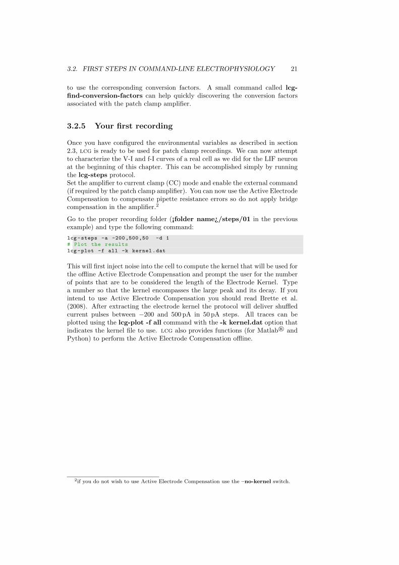
Go to the proper recording folder (¡folder name¿/steps/01 in the previousexample) and type the following command:
‘‘‘‘ ‘‘lcg -steps -a -200,500,50 -d 1
‘‘‘‘ ‘‘# Plot the results
‘‘‘‘ ‘‘lcg -plot -f all -k kernel.dat
This will first inject noise into the cell to compute the kernel that will be used forthe offline Active Electrode Compensation and prompt the user for the numberof points that are to be considered the length of the Electrode Kernel. Typea number so that the kernel encompasses the large peak and its decay. If youintend to use Active Electrode Compensation you should read Brette et al.(2008). After extracting the electrode kernel the protocol will deliver shuffledcurrent pulses between −200 and 500 pA in 50 pA steps. All traces can beplotted using the lcg-plot -f all command with the -k kernel.dat option thatindicates the kernel file to use. lcg also provides functions (for Matlab® andPython) to perform the Active Electrode Compensation offline.
2if you do not wish to use Active Electrode Compensation use the –no-kernel switch.

22 CHAPTER 3. GETTING STARTED
Chapter 4
Electrophysiologyprotocols
In this chapter, we describe the electrophysiology protocols that come withlcg.
All protocols allow the user to specify the sampling frequency (usually witha -F switch, but be careful of exceptions) and the input and output channels(usually with the -I and -O options, respectively, but be extremely careful ofexceptions).
Of the following protocols, only those for the computation of f-I curves witha Proportional-Integral-Derivative (PID) controller and for clamping the fre-quency of a neuron require a real-time kernel. For all other protocols, a Comediinstallation is sufficient.
Note that, whenever in the following voltage clamp or current clamp are men-tioned, lcg does not communicate with the amplifier to switch modes: it is upto the user to do so.
An up-to-date list of the more commonly used protocols can be obtained byentering
‘‘‘‘ ‘‘1 lcg help
4.1 Action potential protocol
This protocol consists in injecting a brief (the default value is 1 ms) depolarizingpulse of current to elicit a single action potential to extract its salient electro-physiological properties. The duration of the pulse should be short enough inorder not to interfere with the actual shape of the action potential. The usercan specify the amplitude and duration of the pulse, as well as the number ofrepetitions and the interval between them.For example, the following command
23

24 CHAPTER 4. ELECTROPHYSIOLOGY PROTOCOLS
‘‘‘‘ ‘‘1 lcg ap -a 2000 -d 1 -n 10 -i 5
injects 10 pulses of amplitude 2000 pA and duration 1 ms with intervals of5 s. The voltage is recorded for 0.5 s before and after the application of thepulse.
4.2 V-I curve protocol
This protocol consists in injecting a series of hyperpolarizing and/or depolarizingsteps of current to compute a V-I curve. The default is to inject steps of currentfrom −300 to 50 pA in steps of 50 pA, which is suited for cortical pyramidalneurons or other large types of cells. Alternatively, the user can specify thevalues of current by using the -a option.For example, the following command
‘‘‘‘ ‘‘1 lcg vi -a -100,40,20 -d 1
instructs the protocol to inject steps of current from −100 to 40 pA in steps of20 pA with a duration of 1 s.
4.3 Time constant protocol
This protocol is identical to the action potential protocol described previously,with the sole exception that the injected pulses of current are hyperpolarizingand can therefore be used to compute the time constant of a cell. The defaultvalues of amplitude and duration of the pulses are −300 pA and 10 ms, but theycan be changed using the -a and -d options, respectively.For example, the command
‘‘‘‘ ‘‘1 lcg tau -n 20
instructs the protocol to inject 20 pulses, instead of the default 30.
4.4 Current ramp protocol
This protocol injects an increasing ramp of current into a cell, to find its thresh-old for spiking. The user can specify the initial and final values of the ramp, aswell as its duration.For example, the command
‘‘‘‘ ‘‘1 lcg ramp -a 50 -A 300 -d 15
instructs the protocol to inject a 15 s ramp, starting from 50 pA and ending at300 pA.

4.5. WHITE NOISE PROTOCOL 25
4.5 White noise protocol
This protocol injects white noise into a cell. It is primarily used to compute theelectrode kernel for the Active Electrode Compensation technique described inBrette et al. (2008).For example, the command
‘‘‘‘ ‘‘1 lcg kernel -s 100
instructs the protocol to inject a noisy trace lasting 10 s, with zero mean andstandard deviation of 100 pA. The default value of standard deviation is 250 pA,which is suited for cortical pyramidal cells. The script also calls lcg-extract-kernelsto extract the electrode kernel and saves the result in a file called kernel.dat.An additional option is provided (-H) to inject an additional holding currentthat is not taken into account in the actual computation of the electrode kernel.This option is useful for spontaneously active cells, like Purkinje cells, or for invivo experiments.
4.6 Filtered noise protocol
This protocol injects a Ornstein-Uhlenbeck process into a cell. It can be usedeither to analyze the reliability and precision of cells, as was done in Mainenand Sejnowski (1995), or to extract the parameters of an exponential integrateand fire model, as described in Badel et al. (2008).For example, the command
‘‘‘‘ ‘‘1 lcg ou -n 20 -i 5 -m 100 -s 100 -t 20 -d 3
instructs the protocol to inject 20 repetitions of a noisy current with mean andstandard deviation equal to 100 pA and time constant of 20 ms. The durationof each injection is 3 s and the interval between repetitions is 5 s.
4.7 Input resistance
This protocol injects a train of hyperpolarizing pulses suited to compute theinput resistance of a cell in vivo, as described in Crochet and Petersen (2006).For example, the command
‘‘‘‘ ‘‘1 lcg rin -a -100 -d 300 -f 1 -D 90
instructs the protocol to inject 300 ms-long pulses of amplitude −100 pA at afrequency of 1 Hz. The total duration of the recording is specified by the -D
option, in this case 90 s. Alternatively, the user can specify, with the -N option,the number of pulses to inject.

26 CHAPTER 4. ELECTROPHYSIOLOGY PROTOCOLS
4.8 DC steps protocol
This protocol injects DC steps of current into a cell, and is a generalization ofthe previously described protocol for the computation of the V-I curve. It hasadditional parameters that allow to specify the duration of the recording afterthe application of the stimulus and an optional holding value.For example, the command
‘‘‘‘ ‘‘1 lcg steps -a 100 ,400 ,50 -d 2 -n 4 -i 5
instructs the protocol to inject steps of current from 100 to 400 pA in steps of50 pA with a duration of 2 s and interval of 5 s. Each amplitude is repeated 4times. Additionally, this protocol has a --vclamp option, which instructs theprogram to consider the steps as voltage ones and use, as a consequence, theappropriate default conversion factors (contained in the .lcg-env.sh file, seeSec. 2.3). In this case, the command
‘‘‘‘ ‘‘1 lcg steps -a -100,0,20 --vclamp
instructs the program to inject voltage steps at values ranging from −100 to0 mV, in steps of 20 mV. For all the other options, default values are used.Note that in both cases, the amplitudes of the steps are shuffled, in order tominimize the effects due to adaptation to increasing (or decreasing) stimulationamplitudes. However, an option is provided (--no-shuffle) to inject the stepsin a linear order.
4.9 f-I curve protocol
Input-output curves, also known as f-I curves, can be easily computed with lcgin two ways: the most straightforward and traditional one is to use lcg-steps
to inject steps of current and subsequently count the number of spikes emittedfor each amplitude.
An alternative way is to use a PID controller and have the neuron follow anincreasing ramp of frequency. The protocol that implements this algorithm islcg-fi, which requires a real-time kernel to operate correctly and can be calledas follows:
‘‘‘‘ ‘‘1 lcg fi -a 150 -m 5 -M 30 -T 30 -n 2 -w 60
which instructs the protocol to initially inject a current of 150 pA and drive thecell from a minimum of 5 to a maximum of 30 Hz. The protocol is repeatedtwice, with each trial lasting 30 s and an interval of 60 s between trials. Notethat here the inter-trial interval option is specified by the -w option, instead ofthe more common -i, which is used, together with -p and -d, to specify theintegral, proportional and derivative gains of the controller, respectively. Notealso that, for optimal results, the initial value of current (150 pA in the example)should be chosen such that it elicits spiking in the cell at a frequency as closeas possible to the minimum required value (here equal to 5 Hz).
4.10. FREQUENCY CLAMP PROTOCOL 27
4.10 Frequency clamp protocol
In a sense, this protocol is the dual of an injection of suprathreshold current:in that case, a constant current is injected (clamped) and the firing frequencyof the cell can be measured. Here, the protocol finds the current necessary tomake the cell spike at a given frequency. To do so, it uses a PID controller inmuch the same way as the protocol for the computation of a f-I curve, with thedifference that here the value of frequency is a constant instead of a ramp.For example, the command
‘‘‘‘ ‘‘1 lcg fclamp -f 10 -a 100
instructs the protocol to clamp the firing frequency of the cell at a value of 10 Hz,starting with an injected current of 100 pA, which must be above threshold, inorder for the frequency estimator to work properly.
4.11 Spontaneous activity protocol
This protocol can be used to record spontaneous activity from an arbitrary num-ber of input channels and is suited both for in vitro and in vivo experiments.The user can specify the duration of the recording, the device, subdevice, chan-nels and gains to be used in the recording. The only limitation is that allchannels need be on the same device and subdevice.For example, the command
‘‘‘‘ ‘‘1 lcg spontaneous -d 60 -I 0,1,2,3
instructs the protocol to record for 60 s from channels 0, 1, 2 and 3. If not speci-fied, the default device file and input subdevice are taken from the .lcg-env.shfile, see Sec. 2.3.
4.12 Train of pulses protocol
This protocol injects a train of brief depolarizing protocols into a cell to elicitaction potentials, while simultaneously recording from two cells, the stimulatedone and another that might be connected to it. The purpose of this protocolis therefore to test the connectivity between pairs of cells and to measure theirshort-term synaptic properties.For example, the command
‘‘‘‘ ‘‘1 lcg pulses -N 8 -O 0 -I 0,1 -f 30 -d 1 -A 3000
instructs the protocol to stimulate a presynaptic cell with a train of 8 pulsesof duration 1 ms and amplitude 3000 pA at a frequency of 30 Hz. The outputchannel (i.e., the channel used to inject current into the presynaptic cell) isnumber 0, while the input channels are numbers 0 and 1, with 0 being the chan-nel connected to the presynaptic cell and 1 that of the postsynaptic cell. Thedefault is to record the presynaptic cell in current clamp and the postsynaptic

28 CHAPTER 4. ELECTROPHYSIOLOGY PROTOCOLS
one in voltage clamp, but the option --cclamp allows to instruct the protocolto record both channels in current clamp mode.
4.13 Utility programs
lcg contains some additional programs that are not protocols, but that canbe used in various occasions during an electrophysiology experiment. They aredescribed in brief in the following, and we refer the user to their help (i.e.,lcg help utility_name) for an in depth description of their options.
• lcg zero outputs zero on all channels of a DAQ board. It is particularlyuseful at the beginning of an experiment, when the output of the DAQboard is undefined.
• lcg output outputs a given value on some channels of the DAQ board.It can be useful when it is required to hold a cell with a certain currentor to a certain voltage, for example in voltage clamp experiments.
• lcg annotate allows the user to add comments into an existing H5 datafile. It accepts two options, -f for the filename and -m for the commentmessage. If no options are specified, the program prompts the user for thefile name and for a message.

Chapter 5
Stimulus generator
Of course, if lcg were restricted only to the protocols described in Chapter 4,it would constitute a cheap replacement of commercial programs such as Pulse,which offer a vast array of additional functionalities. What makes lcg extremelypowerful and versatile is the possibility to define arbitrary stimulus files tobe used in voltage and current clamp experiments, described in this chapter,and the possibility to use configuration files to describe arbitrary experiments,(e.g., dynamic clamp or closed loop experiments) defined as the interactions ofelementary objects. Configuration files and such objects, called entities in thecontext pf lcg, are described in detail in Chapters 7 and 8, respectively. Thischapter describes how to use lcg to inject arbitrary waveforms, described instimulus files.
In principle, all traditional electrophysiology protocols (i.e., those that do notrequire real-time control over the recorded quantities), can be implemented inlcg by using just two commands, lcg-stimgen and lcg-stimulus: the formerproduces stim-files1 according to the specification of the user, and the latterapplies the synthesized waveforms to the appropriate output channels while atthe same time recording from an arbitrary number of input channels.
As a matter of fact, all the protocols described in Chapter 4, with the exceptionof f-I curve and frequency clamp protocols described in Sections 4.9 and 4.10,respectively, can be implemented using only lcg-stimgen and lcg-stimulus.The reason for their existence is simply the possibility to define appropriatedefault values, which make the application of the protocols even simpler.
We will first briefly summarize the rationale behind the meta-language usedto generate stimulation files and then describe how to generate them usinglcg-stimgen and how to use lcg-stimulus to stimulate and record using stim-ulation files.
1The syntax of stim-files is explained in great detail in the companion manual, which mustbe read to properly understand the following instructions.
29

30 CHAPTER 5. STIMULUS GENERATOR
5.1 Stimulation files
Stimulation files, or in short stim-files, are simply text files that contain a piece-wise description of a particular waveform. More in detail, each stim-file is com-posed of a certain number of lines, with each line representing an elementarysub-waveform: the full waveform is therefore given by the concatenation of allsub-waveforms. Each elementary sub-waveform is described by 12 coefficients:
T code p1 p2 p3 p4 p5 fix-seed seed subcode op exp
The meaning of the coefficients is the following:
T duration of the sub-waveformcode code that identifies the sub-waveform
p1, . . . , p5 parameters that specify the sub-waveformfix-seed whether or not the seed should be fixed (only for stochastic sub-waveforms)
seed the seed to use (only for stochastic sub-waveforms)subcode the code of another sub-waveform, if algebraic operations are to be performed
op the algebraic operation to performexp the exponent to which the sub-waveform should be raised
Available codes range from 1 to 12 and identify 12 different types of elementarysub-waveforms, such as constants, sinusoids, square waves, Ornstein-Uhlenbeckstochastic process realizations, and so on. The full list of available waveformsis described in detailed in the companion manual, which can be found at http://danielelinaro.github.io/dynclamp/stimgen_manual.pdf.
If a noisy waveform is to be used, it is possible to set the seed used in thegeneration of the pseudo-random numbers. It is also possible to specify whetherthe seed should be used or not: in the latter case, a random seed is generatedusing the device /dev/random, available on most UNIX systems.
As mentioned previously, sub-waveforms can be combined to yield more com-plex stimulation waveforms: this is not limited only to the concatenation ofelementary sub-waveforms, but can be implemented also by applying algebraicoperations to sets of sub-waveforms. The way this is achieved is described inthe companion manual.
Finally, each elementary sub-waveform can be raised to a particular exponent(for example 0.5 to obtain the square root of a waveform): this is achieved bysetting the appropriate value for the last parameter of the sub-waveform.
This description of stimulus files is by no means exhaustive: we strongly encour-age readers to familiarize themselves with the definition of stimulation wave-forms by reading carefully through the companion manual.
5.2. GENERATING STIMULATION FILES 31
5.2 Generating stimulation files
As mentioned previously, stimulation files can be generated in lcg using thecommand lcg-stimgen: this provides a convenient interface to the stim-filelanguage, and saves the user the hassle of having to write stim-files manually.Also, it provides a way of interacting directly with lcg-stimulus by feedingthe output of lcg-stimgen to lcg-stimulus by means of UNIX pipes, as willbe described in the following section.
The syntax of lcg-stimgen is the following:
lcg-stimgen -o|--output filename [-a|--append]
<waveform_1> [option <value>] p_1 p_2 ... p_5
<waveform_2> [option <value>] p_1 p_2 ... p_5
...
<waveform_N> [option <value>] p_1 p_2 ... p_5
Since lcg-stimgen can deal with an arbitrary number of waveforms, the op-tions that specify the output file name (-o or --output switches) and whetherthe output should be appended to an existing file (-a or --append switches)should precede the definition of any sub-waveform. If no output file is specified,lcg-stimgen will output the resulting stim-file to standard output: this is use-ful both for testing purposes and for usage in conjuction with lcg-stimulus aswill be described in the following.
Next comes the specification of each single sub-waveform with its parameters:the first parameter (i.e, waveform_1, waveform_2 and so on) is a code thatrepresent the type of waveform. At present, the accepted codes are dc, ou, sine,square, saw, chirp, ramp, poisson-reg, poisson-exp, poisson-bi, gaussian,alpha. For the meaning of each one, see the companion manual. The optionalarguments for each sub-waveform are the following:
-d duration of the sub-waveform in seconds-s seed of the sub-waveform, also sets fix-seed accordingly-e exponent of the sub-waveform-p sum this sub-waveform and the following
-m subtract the following sub-waveform from this one-M multiply this sub-waveform and the following-D divide this sub-waveform by the following-E compute the composite waveform: this option is required for the last waveform in a series
Every short option has a corresponding long one, detailed in the online help oflcg-stimgen, accessible by issuing at a prompt the following command:
‘‘‘‘ ‘‘1 lcg -stimgen -h
Additionally, all other options —except for the duration— have default values,which are also detailed in the online help of the command.
The positional arguments p_1 to p_5 come after the optional arguments. Eachwaveform requires a certain number of parameters: for instance, the constantwaveform requires just one parameter, whereas a sinusoidal waveform requires

32 CHAPTER 5. STIMULUS GENERATOR
4. The exact number of parameters required by each sub-waveform is accessibleby issuing the command
‘‘‘‘ ‘‘1 lcg -stimgen help <code >
where code is one of the sub-waveform codes described before: for example, thecommand
‘‘‘‘ ‘‘1 lcg -stimgen help sine
produces the following output:
Waveform ‘sine’ takes 4 parameters:
1) amplitude
2) frequency (Hz)
3) phase
4) offset
Note that, according to the argument passing convention on UNIX systems, ifone of the positional arguments (i.e., one of the parameters of a sub-waveform)is negative (e.g., a negative amplitude in a constant sub-waveform), the full listof positional arguments should be preceded by a double minus sign, as in
‘‘‘‘ ‘‘1 lcg -stimgen -o negative.stim dc -d 1 -- -100
5.2.1 Examples
The following commands generate the stimulus files presented in the companionmanual as examples.
Example 1: a positive 5 s-long step preceded and followed by a 2.5 s-long con-stant of 0.
‘‘‘‘ ‘‘1 lcg -stimgen dc -d 2.5 0 dc -d 5 2 dc -d 2.5 0
Example 2: a negative 5 s-long step preceded and followed by a 2.5 s-longconstant of 0. Note the double minus sign used to delimit the beginning of thepositional arguments, when at least one of them is negative.
‘‘‘‘ ‘‘1 lcg -stimgen dc -d 2.5 0 dc -d 5 -- -2 dc -d 2.5 0
Example 3: 2 200 ms-long Ornsteing-Uhlenbeck waveforms with different meaninterleaved by constant waveforms.
‘‘‘‘ ‘‘1 lcg -stimgen dc -d 0.1 0 ou -d 0.2 -- -2 0.5 1 dc -d 0.05 0 ou -d
‘‘‘‘ ‘‘0.2 2 0.5 1 dc -d 0.1 0
Example 4: 2 200 ms-long Ornsteing-Uhlenbeck waveforms with different timeconstants interleaved by constant waveforms.
‘‘‘‘ ‘‘1 lcg -stimgen dc -d 0.1 0 ou -d 0.2 2 0.5 1 dc -d 0.05 0 ou -d 0.2 2
‘‘‘‘ ‘‘0.5 10 dc -d 0.1 0
Example 5: 3 200 ms-long Ornsteing-Uhlenbeck waveforms with identical pa-rameters. The first two also have the same seed, whereas the third one has noseed specified.

5.2. GENERATING STIMULATION FILES 33
‘‘‘‘ ‘‘1 lcg -stimgen dc -d 0.1 0 ou -d 0.2 -s 21 2 0.5 100 dc -d 0.05 0 ou -
‘‘‘‘ ‘‘d 0.2 -s 21 2 0.5 100 dc -d 0.05 0 ou -d 0.2 2 0.5 100 dc -d
‘‘‘‘ ‘‘0.1 0
Example 6: a 5 s-long sinusoidal waveform.
‘‘‘‘ ‘‘1 lcg -stimgen dc -d 2.5 0 sine -d 5 3 1 0 0 dc -d 2.5 0
Example 7: a 5 s-long square waveform.
‘‘‘‘ ‘‘1 lcg -stimgen dc -d 2.5 0 square -d 5 3 1 50 dc -d 2.5 0
Example 8: a 5 s-long saw-tooth waveform.
‘‘‘‘ ‘‘1 lcg -stimgen dc -d 2.5 0 saw -d 5 3 1 50 dc -d 2.5 0
Example 9: a 5 s-long chirp waveform.
‘‘‘‘ ‘‘1 lcg -stimgen dc -d 2.5 0 chirp -d 5 4 1 10 dc -d 2.5 0
Example 10: a 5 s-long ramp waveform. Note that the ramp waveform startsat the last value of the previous waveform (or zero, if there is no sub-waveformpreceding the ramp) and ends at the value specified as a parameter, whichtherefore does not necessarily represent the total span of the ramp.
‘‘‘‘ ‘‘1 lcg -stimgen dc -d 2.5 -1 ramp -d 5 4 dc -d 2.5 4
Example 11: unipolar 1.5 ms-long square pulses of amplitude 4 delivered at afrequency of 10 Hz.
‘‘‘‘ ‘‘1 lcg -stimgen dc -d 0.5 0 poisson -reg -d 1 -- 4 -10 1.5 dc -d 0.5 0
Example 12: exponential pulses with a decay time constant of 5 ms and am-plitude 4 delivered at a frequency of 10 Hz.
‘‘‘‘ ‘‘1 lcg -stimgen dc -d 0.5 0 poisson -exp -d 1 -- 4 -10 5 dc -d 0.5 0
Example 13: bipolar 5 ms-long square pulses of amplitude 4 delivered at afrequency of 10 Hz.
‘‘‘‘ ‘‘1 lcg -stimgen dc -d 0.5 0 poisson -bi -d 1 -- 4 -10 5 dc -d 0.5 0
Example 14: same as example 13, with the difference that here the pulsesare not delivered regularly, but rather they are generated by an exponentialdistribution with mean rate equal to 10 Hz.
‘‘‘‘ ‘‘1 lcg -stimgen dc -d 0.5 0 poisson -bi -d 1 4 10 5 dc -d 0.5 0
Example 15: three “bursts” of unipolar square pulses whose occurrence timesare exponentially distributed. The first two bursts have the same seed (there-fore producing the same sequence of events), while the third burst has no seedspecified.
‘‘‘‘ ‘‘1 lcg -stimgen dc -d 0.5 0 poisson -reg -d 1 -s 43 4 10 5 dc -d 0.5 0
‘‘‘‘ ‘‘poisson -reg -d 1 -s 43 4 10 5 dc -d 0.5 0 poisson -reg -d 1 4 10
‘‘‘‘ ‘‘5 dc -d 0.5 0
Example 16: alpha function waveform.
34 CHAPTER 5. STIMULUS GENERATOR
‘‘‘‘ ‘‘1 lcg -stimgen dc -d 0.5 0 alpha -d 1 4 15 50 200 dc -d 0.5 0
Example 17: a rectified sinusoidal waveform. This can be accomplished bysetting the exponent parameter to -1, which effectively takes the absolute value,point by point, of the original elementary sub-waveform.
‘‘‘‘ ‘‘1 lcg -stimgen dc -d 0.5 0 sine -d 5 -e -1 4 1 0 0 dc -d 0.5 1
Example 18: positive part of a sinusoidal waveform. This can be accomplishedby setting the exponent parameter to 0, which takes, point by point, the positivepart of the original elementary sub-waveform.
‘‘‘‘ ‘‘1 lcg -stimgen dc -d 0.5 0 sine -d 5 -e 0 4 1 0 0 dc -d 0.5 1
Example 19: sum of a sinusoidal and a Ornstein-Uhlenbeck waveform.
‘‘‘‘ ‘‘1 lcg -stimgen dc -d 0.5 0 sine -d 5 -p 1 1 0 0 ou -E 0 0.2 5 dc -d
‘‘‘‘ ‘‘0.5 0
Example 20: product of a sinusoidal and a Ornstein-Uhlenbeck waveform.
‘‘‘‘ ‘‘1 lcg -stimgen dc -d 0.5 0 sine -d 5 -M 1 1 0 0 ou -E 0 0.2 5 dc -d
‘‘‘‘ ‘‘0.5 0

Chapter 6
Data files
In this chapter we describe the structure of the H5 files used by lcg to storethe recorded data.
35

36 CHAPTER 6. DATA FILES
Infoversion
dttend
tStartSec
tStartNSec
Events
Code Sender Timestamp
Entities
0001Name
Units
Data Parameters Metadata
0002 000N
Figure 6.1: Diagram of the data file model implemented with the H5Recorder.
Chapter 7
Configuration files
This chapter describes how to write custom configuration files to be used bylcg.
7.1 Introduction
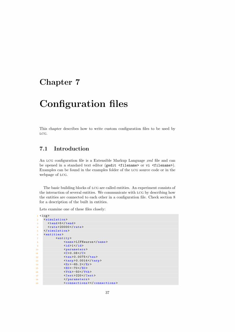
An lcg configuration file is a Extensible Markup Language xml file and canbe opened in a standard text editor (gedit <filename> or vi <filename>).Examples can be found in the examples folder of the lcg source code or in thewebpage of lcg.
The basic building blocks of lcg are called entities. An experiment consists ofthe interaction of several entities. We communicate with lcg by describing howthe entities are connected to each other in a configuration file. Check section 8for a description of the built in entities.
Lets examine one of these files closely:
‘‘‘‘ ‘‘1 <lcg>
‘‘‘‘ ‘‘2 <simulation >
‘‘‘‘ ‘‘3 <tend>5</tend>
‘‘‘‘ ‘‘4 <rate>20000</rate>
‘‘‘‘ ‘‘5 </simulation >
‘‘‘‘ ‘‘6 <entities >
‘‘‘‘ ‘‘7 <entity >
‘‘‘‘ ‘‘8 <name>LIFNeuron </name>
‘‘‘‘ ‘‘9 <id>1</id>
‘‘‘‘ ‘‘10 <parameters >
‘‘‘‘ ‘‘11 <C>0.08</C>
‘‘‘‘ ‘‘12 <tau>0.0075 </tau>
‘‘‘‘ ‘‘13 <tarp>0.0014 </tarp>
‘‘‘‘ ‘‘14 <Er> -65.2</Er>
‘‘‘‘ ‘‘15 <E0> -70</E0>
‘‘‘‘ ‘‘16 <Vth> -50</Vth>
‘‘‘‘ ‘‘17 <Iext>220</Iext>
‘‘‘‘ ‘‘18 </parameters >
‘‘‘‘ ‘‘19 <connections ></connections >
37

38 CHAPTER 7. CONFIGURATION FILES
‘‘‘‘ ‘‘20 </entity >
‘‘‘‘ ‘‘21 </entities >
‘‘‘‘ ‘‘22 </lcg>
Example 7.1: A simple example of a configuration file with a simulated integrateand fire neuron.
This file is composed layers. The most general is the <lcg> layer; this basicallytells the program that this is a configuration file. Inside this layer there are twoother:
• <simulation> - where the general parameters are defined e.g. the sam-pling rate (rate) and the duration (tend).
• <entities> - where the entities are listed and connected to each other.Generally each <entity> has a
– <name> - the global descriptor of the entitiy.
– <id> - the global identification number of an entity. This is used toconnect entities and the ids have to be unique.
– <parameters> - the parameters of the entity. These vary betweeneach entity. You can use the manual section 8.
– <connections> - the global ids to which this entity is connected.
Now lets create a file called example.xml. Open a terminal and copy thefollowing lines one by one:
‘‘‘‘ ‘‘1 mkdir ~/ examples # this creates a directory called under your home
‘‘‘‘ ‘‘folder (that ’s what the tilt is for)
‘‘‘‘ ‘‘2 cd ~/ examples # goes inside this directory
‘‘‘‘ ‘‘3 gedit example1.xml # creates and opens a file called example.xml in
‘‘‘‘ ‘‘the current folder using gnome text editor.
Note that if you do have a system without gnome like Mac OS the commandgedit will not work; any text editor can be used. Now copy the example (7.1)above to this file. If you use copy and paste make sure that there are no extraspaces, this will depend on the your choice of editor. Save and close it. Youcan now run the example by doing: lcg -c example.xml
The -c option stands for configuration file can be used to tell lcg that weare going to pass a configuration file as an argument.
You have just ran a simulation of an integrate and fire neuron’s membranepotential for 5 seconds. This was a very basic example, so the data was notrecorded since there is no recording entity.
Chapter 8
Entities
Entities are one of the basic building blocks of real-time experiments with lcg.As mentioned in chapter 7, experiments are described in configuration files (thatfollow the XML standard) where entities are described and connected. Complexprotocols can be designed by combining entities in different ways.
Going a little bit in the design of the entities, in its essence, these are C++classes with particular defined methods that let them interface in the same waywith the experiment engine. These methods are:
• initialise() - where the initial parameters of the entity are set as well asthe initial input.
• firstStep() - executed in the first step of the experiment (where parametersthat depend on precise timing can be initialised).
• step() - that is executed at every timestep of the simulation/experiment.
• handleEvent() - that is executed every time an event is received by theentity.
• terminate() - that is executed when the simulation/experiment ends.
Aside of the above described methods, entities have access to the outputs of allentities they are connected to and have an output of themselves. The output isnonetheless than a single double value that changes (or not) at every time-stepdepending on either the step() or the handleEvent() methods.
This chapter describes the entities contained in lcg, it provides short defini-tions of entity and the general properties. The descriptions can be used tocreate configuration files, however there are also Python helper classes to createconfiguration files. The helper classes are the ones used by most protocols andits usage is encouraged.
39
40 CHAPTER 8. ENTITIES
8.1 H5Recorder
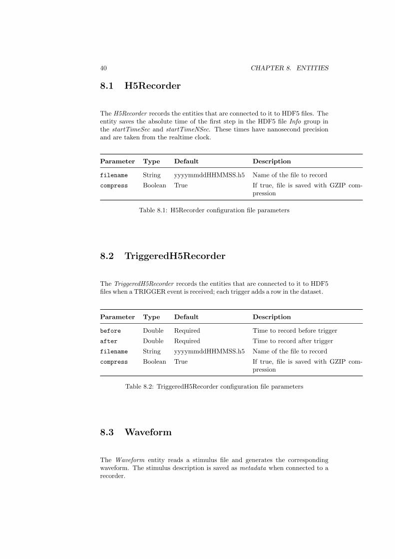
The H5Recorder records the entities that are connected to it to HDF5 files. Theentity saves the absolute time of the first step in the HDF5 file Info group inthe startTimeSec and startTimeNSec. These times have nanosecond precisionand are taken from the realtime clock.
Parameter Type Default Description
filename String yyyymmddHHMMSS.h5 Name of the file to record
compress Boolean True If true, file is saved with GZIP com-pression
Table 8.1: H5Recorder configuration file parameters
8.2 TriggeredH5Recorder
The TriggeredH5Recorder records the entities that are connected to it to HDF5files when a TRIGGER event is received; each trigger adds a row in the dataset.
Parameter Type Default Description
before Double Required Time to record before trigger
after Double Required Time to record after trigger
filename String yyyymmddHHMMSS.h5 Name of the file to record
compress Boolean True If true, file is saved with GZIP com-pression
Table 8.2: TriggeredH5Recorder configuration file parameters
8.3 Waveform
The Waveform entity reads a stimulus file and generates the correspondingwaveform. The stimulus description is saved as metadata when connected to arecorder.
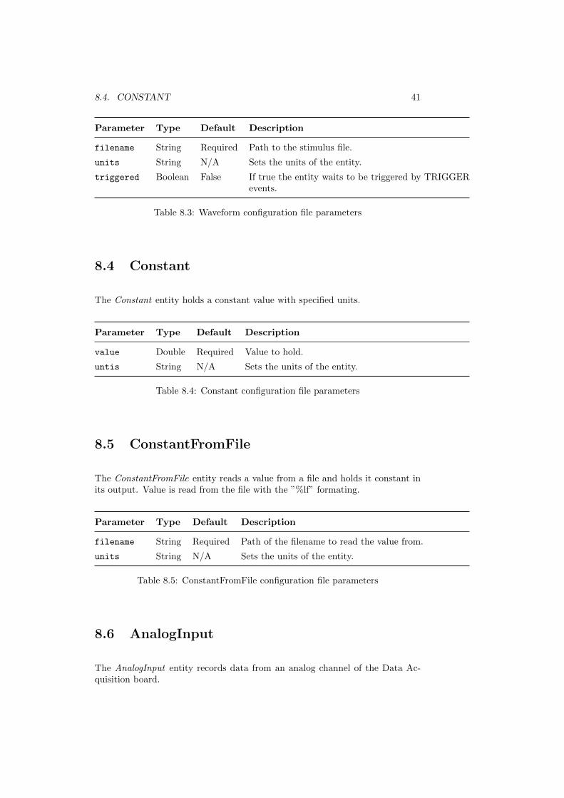
8.4. CONSTANT 41
Parameter Type Default Description
filename String Required Path to the stimulus file.
units String N/A Sets the units of the entity.
triggered Boolean False If true the entity waits to be triggered by TRIGGERevents.
Table 8.3: Waveform configuration file parameters
8.4 Constant
The Constant entity holds a constant value with specified units.
Parameter Type Default Description
value Double Required Value to hold.
untis String N/A Sets the units of the entity.
Table 8.4: Constant configuration file parameters
8.5 ConstantFromFile
The ConstantFromFile entity reads a value from a file and holds it constant inits output. Value is read from the file with the ”%lf” formating.
Parameter Type Default Description
filename String Required Path of the filename to read the value from.
units String N/A Sets the units of the entity.
Table 8.5: ConstantFromFile configuration file parameters
8.6 AnalogInput
The AnalogInput entity records data from an analog channel of the Data Ac-quisition board.

42 CHAPTER 8. ENTITIES
Parameter Type Default Description
deviceFile String Required Device File (example /dev/-comedi0 to record from the firstcomedi board).
inputSubdevice Integer Required Subdevice (needs to be an analoginput subdevice)
readChannel Integer Required Input channel to read from.
inputConversionFactor Double Required Conversion factor associated withthe quantity being measured.
range String [-10,+10] Input range to control the boardinternal gains.
reference String GRSE or NRSE Refers to the grounding schemebeing used, check the board man-ual.
units String mV Units after conversion.
Table 8.6: AnalogInput configuration file parameters
8.7 AnalogOutput
The AnalogOutput entity outputs data to an analog channel of the Data Acqui-sition board.
Parameter Type Default Description
deviceFile String Required Device File (example /dev/-comedi0 to record from the firstcomedi board).
ouputSubdevice Integer Required Subdevice (needs to be an analogoutput subdevice)
writeChannel Integer Required Output channel to write to.
outputConversionFactor Double Required Conversion factor associated withthe quantity being output.
range String [-10,+10] Output range to control theboard internal gains.
reference String GRSE or NRSE Refers to the grounding schemebeing used, check the board man-ual.
units String mV Units after conversion.
Table 8.7: AnalogOutput configuration file parameters

8.8. ANALOGIO 43
8.8 AnalogIO
The AnalogIO entity that combines entities 8.6 and 8.7. Reads from an inputchannel and outputs what is connected to it to an analog channel of the DataAcquisition board.
Parameter Type Default Description
deviceFile String Required Device File (example /dev/-comedi0 to record from the firstcomedi board).
inputSubdevice Integer Required Subdevice (needs to be an analoginput subdevice)
readChannel Integer Required Input channel to read from.
inputConversionFactor Double Required Conversion factor associated withthe quantity being measured.
inputRange String [-10,+10] Output range to control theboard internal gains.
reference String GRSE or NRSE Refers to the grounding schemebeing used, check the board man-ual.
units String mV Input units after conversion.
ouputSubdevice Integer Required Subdevice (needs to be an analogoutput subdevice)
writeChannel Integer Required Output channel to write to.
outputConversionFactor Double Required Conversion factor associated withthe quantity being output.
Table 8.8: AnalogIO configuration file parameters
8.9 RealNeuron
The RealNeuron entity that combines entities 8.6 and 8.7 and is able to performActive Electrode Compensation Online Brette et al. (2008). Emits spikes uponthreshold crossing.
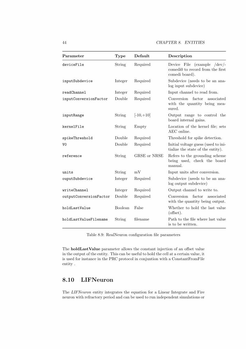
44 CHAPTER 8. ENTITIES
Parameter Type Default Description
deviceFile String Required Device File (example /dev/-comedi0 to record from the firstcomedi board).
inputSubdevice Integer Required Subdevice (needs to be an ana-log input subdevice)
readChannel Integer Required Input channel to read from.
inputConversionFactor Double Required Conversion factor associatedwith the quantity being mea-sured.
inputRange String [-10,+10] Output range to control theboard internal gains.
kernelFile String Empty Location of the kernel file; setsAEC online.
spikeThreshold Double Required Threshold for spike detection.
V0 Double Required Initial voltage guess (used to ini-tialize the state of the entity).
reference String GRSE or NRSE Refers to the grounding schemebeing used, check the boardmanual.
units String mV Input units after conversion.
ouputSubdevice Integer Required Subdevice (needs to be an ana-log output subdevice)
writeChannel Integer Required Output channel to write to.
outputConversionFactor Double Required Conversion factor associatedwith the quantity being output.
holdLastValue Boolean False Whether to hold the last value(offset).
holdLastValueFilename String filename Path to the file where last valueis to be written.
Table 8.9: RealNeuron configuration file parameters
The holdLastValue parameter allows the constant injection of an offset valuein the output of the entity. This can be useful to hold the cell at a certain value, itis used for instance in the PRC protocol in conjuntion with a ConstantFromFileentity .
8.10 LIFNeuron
The LIFNeuron entity integrates the equation for a Linear Integrate and Fireneuron with refractory period and can be used to run independent simulations or

8.11. IZHIKEVICHNEURON 45
to interface simulated neurons with real cells. It is often used also for debugingof complex protocols.
Parameter Type Default Description
C Double Required Cell membrane capacitance.
tau Double Required Cell membrane time constant.
tarp Double Required Refractory period.
Er Double Required Reset potential.
E0 Double Required Equilibrium potential.
Vth Double Required Threshold for spike emission.
Iext Double Required External current offset.
holdLastValue Boolean False Whether to hold the last value (offset).
holdLastValueFilename String filename File where last value is written.
Table 8.10: LIFNeuron configuration file parameters
8.11 IzhikevichNeuron
The IzhickevichNeuron entity integrates the equation for a Izhickevich neuronwith refractory period and can be used to run independent simulations or tointerface simulated neurons with real cells; similarly to entity 8.10. It is oftenused also for debuging of complex protocols.
Parameter Type Default Description
a Double 0.02 a parameter.
b Double 0.2 b parameter.
c Double -65 c parameter.
d Double 2 d parameter.
Vspk Double 30 Spike voltage value.
Iext Double 0 External current offset.
Table 8.11: IzhickevichNeuron configuration file parameters
8.12 FrequencyEstimator
The FrequencyEstimator entity estimates the instantaneous frequency of anevent by iterating the following formula:
Fk = tk−1 ·
(1 − e−tk/τ)
)+ Fk−1 · e−tk/τ , (8.1)

46 CHAPTER 8. ENTITIES
where tk is the time of the kth event and τ (in s) the time scale over which theinstantaneous event rate is estimated, weighing each new event time and the pre-vious event rate history Fk−1 Wallach et al. (2011); Linaro et al. (2014).
Parameter Type Default Description
tau Double Required Estimator time constant.
initialFrequency Double 0.0 Initial frequency estimation (Fk−1).
Table 8.12: FrequencyEstimator configuration file parameters
8.13 PID
The PID entity is evolved by TRIGGER or SPIKE events, here referred bytriggers. The output of the entity is kept constant between triggers. Further-more, it can be set ON or OFF by a TOGGLE event; when OFF, the triggershave no effect on the output of the entity.
The entity requires two inputs; the inputs are compared to yield the errorsignal ek = input2 − input1. The output of the PID is then updated at everytrigger by the equation:
Ik holding = gP · ek + gI ·k∑i=0
ei + gD · (ek − ek−1), (8.2)
where gP , gI , gD are the proportional, integral, and derivative gains, respec-tively.
Parameter Type Default Description
gp Double Required Proportional gain.
gi Double Required Integral gain.
gd Double 0.0 Derivative gain.
Table 8.13: PID configuration file parameters
8.14 EventCounter
The EventCounter entity counts events received and emits events when a certaincount is reached. It can be used to trigger or toggle other entities or to stop theexperiment/simulation.
lcg currently implements the following events:
1. SPIKE - Signal a spike in a Neuron.
2. TRIGGER - Trigger other entities.
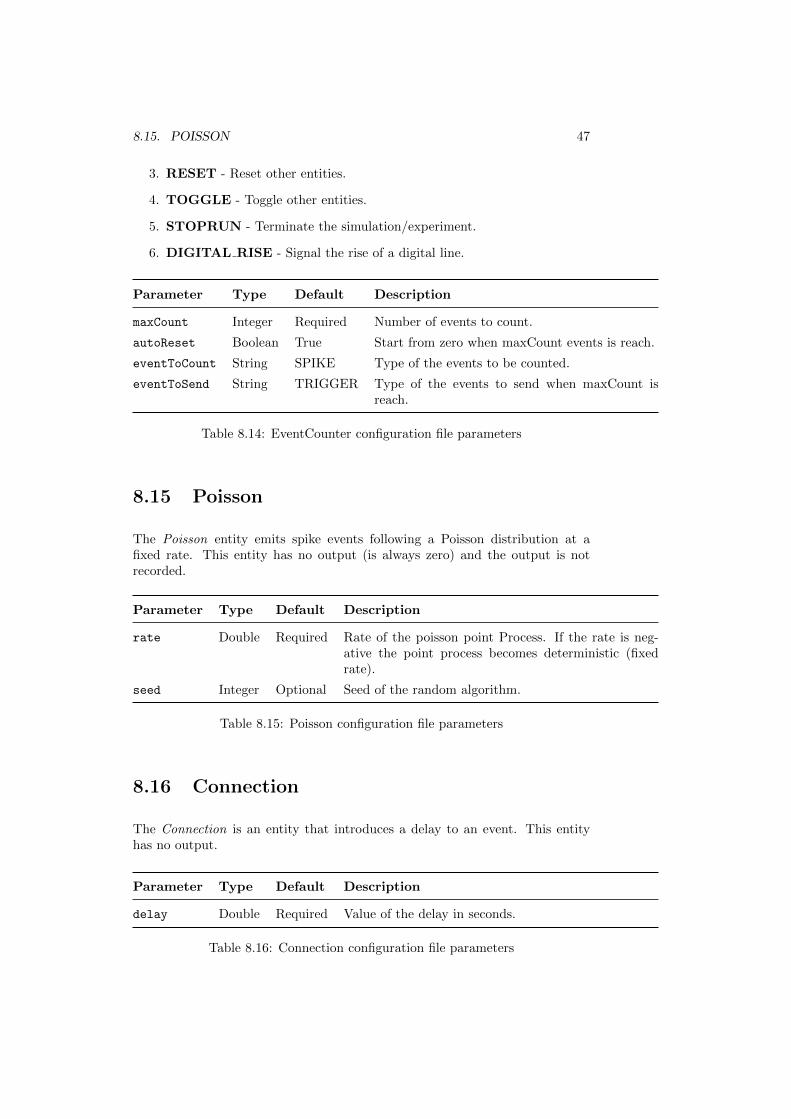
8.15. POISSON 47
3. RESET - Reset other entities.
4. TOGGLE - Toggle other entities.
5. STOPRUN - Terminate the simulation/experiment.
6. DIGITAL RISE - Signal the rise of a digital line.
Parameter Type Default Description
maxCount Integer Required Number of events to count.
autoReset Boolean True Start from zero when maxCount events is reach.
eventToCount String SPIKE Type of the events to be counted.
eventToSend String TRIGGER Type of the events to send when maxCount isreach.
Table 8.14: EventCounter configuration file parameters
8.15 Poisson
The Poisson entity emits spike events following a Poisson distribution at afixed rate. This entity has no output (is always zero) and the output is notrecorded.
Parameter Type Default Description
rate Double Required Rate of the poisson point Process. If the rate is neg-ative the point process becomes deterministic (fixedrate).
seed Integer Optional Seed of the random algorithm.
Table 8.15: Poisson configuration file parameters
8.16 Connection
The Connection is an entity that introduces a delay to an event. This entityhas no output.
Parameter Type Default Description
delay Double Required Value of the delay in seconds.
Table 8.16: Connection configuration file parameters

48 CHAPTER 8. ENTITIES
8.17 VariableDelayConnection
The VariableDelayConnection is an entity that introduces a delay to an event.This entity has no output and no parameters, the behavior is dictated by theoperators connected to it: see entities PhasicDelay, SobolDelay and RandomDe-lay.
8.18 SynapticConnection
The SynapticConnection is an entity that introduces a delay to a SPIKE eventwith synaptic weight. This entity has no output.
Parameter Type Default Description
delay Double Required Value of the delay in seconds.
weight Double Required Weight of the synapse.
Table 8.17: SynapticConnection configuration file parameters
8.19 PhasicDelay
The PhasicDelay is a special type of entity (functor) that returns the inputmultiplied by a constant value. It can be used for instance to give the phase inan slightly noisy oscillatory cycle. This entity has no output.
Parameter Type Default Description
delay Double 0.0 Value of the delay (usually between zero and one)
Table 8.18: PhasicDelay configuration file parameters
8.20 SobolDelay
The SobolDelay is a special type of entity (functor) that returns numbers drawnfrom a Sobol Pseudo-Random distribution multiplied by the input to the entity.Its used for instance in the PRC protocol, use the --dry-run switch for anexample. This entity has no output.
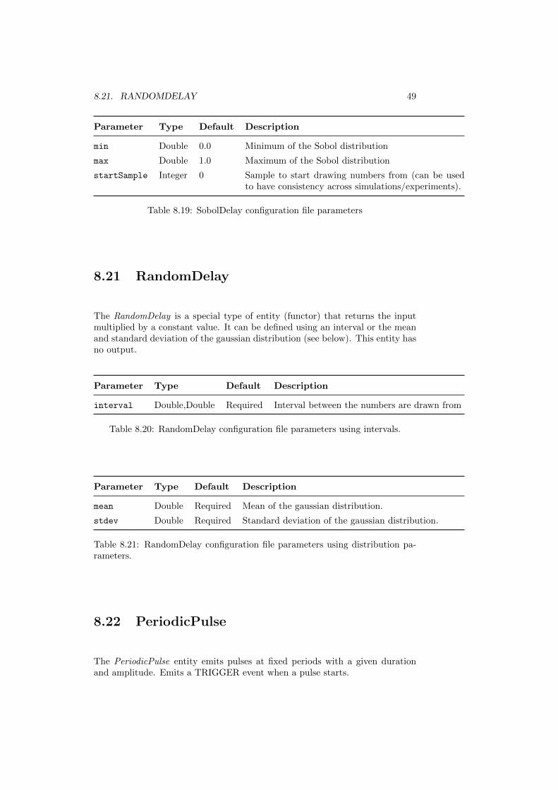
8.21. RANDOMDELAY 49
Parameter Type Default Description
min Double 0.0 Minimum of the Sobol distribution
max Double 1.0 Maximum of the Sobol distribution
startSample Integer 0 Sample to start drawing numbers from (can be usedto have consistency across simulations/experiments).
Table 8.19: SobolDelay configuration file parameters
8.21 RandomDelay
The RandomDelay is a special type of entity (functor) that returns the inputmultiplied by a constant value. It can be defined using an interval or the meanand standard deviation of the gaussian distribution (see below). This entity hasno output.
Parameter Type Default Description
interval Double,Double Required Interval between the numbers are drawn from
Table 8.20: RandomDelay configuration file parameters using intervals.
Parameter Type Default Description
mean Double Required Mean of the gaussian distribution.
stdev Double Required Standard deviation of the gaussian distribution.
Table 8.21: RandomDelay configuration file parameters using distribution pa-rameters.
8.22 PeriodicPulse
The PeriodicPulse entity emits pulses at fixed periods with a given durationand amplitude. Emits a TRIGGER event when a pulse starts.

50 CHAPTER 8. ENTITIES
Parameter Type Default Description
frequency Double Required Frequency of the pulses.
duration Double Required Sets the duration of the pulses (in seconds).
amplitude Double Required Sets the amplitude of the pulses.
units String pA Units of the output.
Table 8.22: PeriodicPulse configuration file parameters
8.23 PeriodicTrigger
The PeriodicTrigger entity emits trigger events with a fixed period.
Parameter Type Default Description
frequency Double Required Frequency of the triggers.
delay Double 0 Sets the Delay of the first trigger.
tend Double INFINITY Sets the maximum time of the last trigger.
Table 8.23: PeriodicTrigger configuration file parameters
8.24 ExponentialSynapse
The ExponentialSynapse entity models a synapse as a single exponential. Needsto be connected to a Neuron and injects a conductance. Spike events increasethe weight of the synapse.
Parameter Type Default Description
E Double Required Reversal Potential.
tau Double Required Time constant.
Table 8.24: ExponentialSynapse configuration file parameters
8.25 Exp2Synapse
The Exp2Synapse entity models a synapse as a alpha function. Needs to beconnected to a Neuron and injects a conductance. Spike events increase theweight of the synapse.
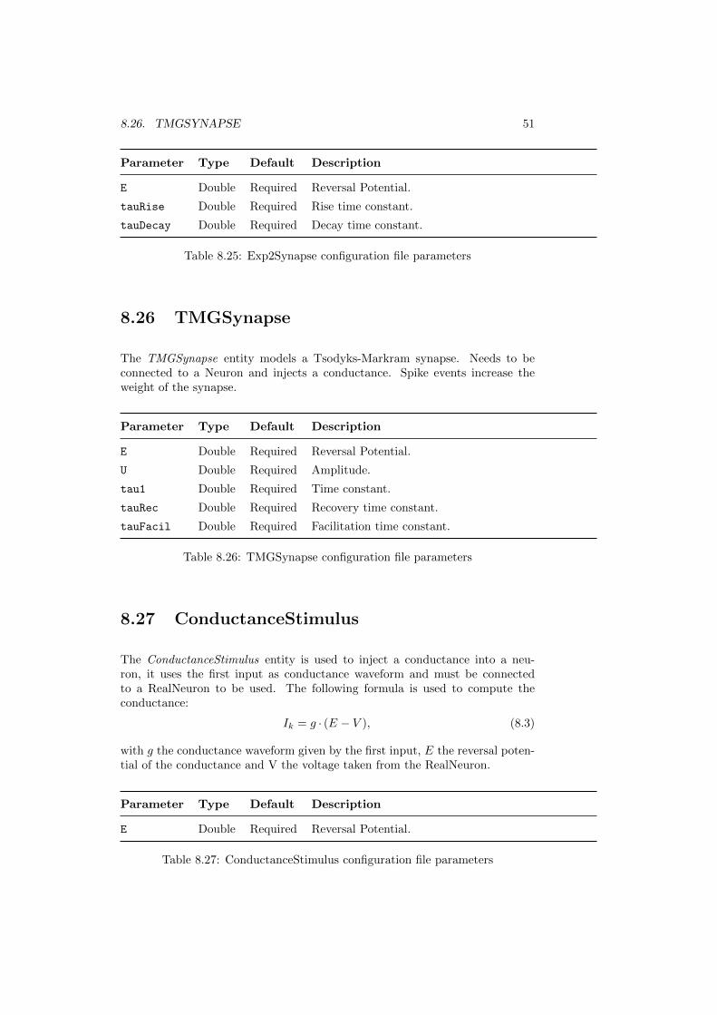
8.26. TMGSYNAPSE 51
Parameter Type Default Description
E Double Required Reversal Potential.
tauRise Double Required Rise time constant.
tauDecay Double Required Decay time constant.
Table 8.25: Exp2Synapse configuration file parameters
8.26 TMGSynapse
The TMGSynapse entity models a Tsodyks-Markram synapse. Needs to beconnected to a Neuron and injects a conductance. Spike events increase theweight of the synapse.
Parameter Type Default Description
E Double Required Reversal Potential.
U Double Required Amplitude.
tau1 Double Required Time constant.
tauRec Double Required Recovery time constant.
tauFacil Double Required Facilitation time constant.
Table 8.26: TMGSynapse configuration file parameters
8.27 ConductanceStimulus
The ConductanceStimulus entity is used to inject a conductance into a neu-ron, it uses the first input as conductance waveform and must be connectedto a RealNeuron to be used. The following formula is used to compute theconductance:
Ik = g · (E − V ), (8.3)
with g the conductance waveform given by the first input, E the reversal poten-tial of the conductance and V the voltage taken from the RealNeuron.
Parameter Type Default Description
E Double Required Reversal Potential.
Table 8.27: ConductanceStimulus configuration file parameters

52 CHAPTER 8. ENTITIES
8.28 NMDAConductanceStimulus
The NMDAConductanceStimulus entity is used to inject an NMDA conductanceinto a neuron, it uses the first input as conductance waveform and must beconnected to a RealNeuron to be used (like entity 8.27 ). The following formulais used to compute the conductance:
Ik =g · (E − V )
1 +K1 · exp−K2 ·V , (8.4)
with g the conductance waveform given by the first input, E the reversal poten-tial of the conductance and V the voltage taken from the RealNeuron.
Parameter Type Default Description
E Double Required Reversal Potential.
K1 Double Required NMDA amplitude.
K2 Double Required NMDA time constant.
Table 8.28: ConductanceStimulus configuration file parameters
8.29 OU
The OU entity outputs an Ornstein-Uhlenbeck fluctuating waveform with staticmean, standard deviation and time constant.
Parameter Type Default Description
mean Mean Required Sets the mean of the OU process.
stdev Double Required Sets the standard deviation of the OUprocess.
tau Double Required Sets the time constant of the OU pro-cess.
units String Required Sets the units of the entity.
initialCondition Double Required Sets the initial Condition.
interval Double,Double Required Sets the interval.
Table 8.29: OU configuration file parameters
8.30 OUNonStationary
The OUNonStationary entity outputs an Ornstein-Uhlenbeck fluctuating wave-form with mean and standard deviation taken from the first two inputs.
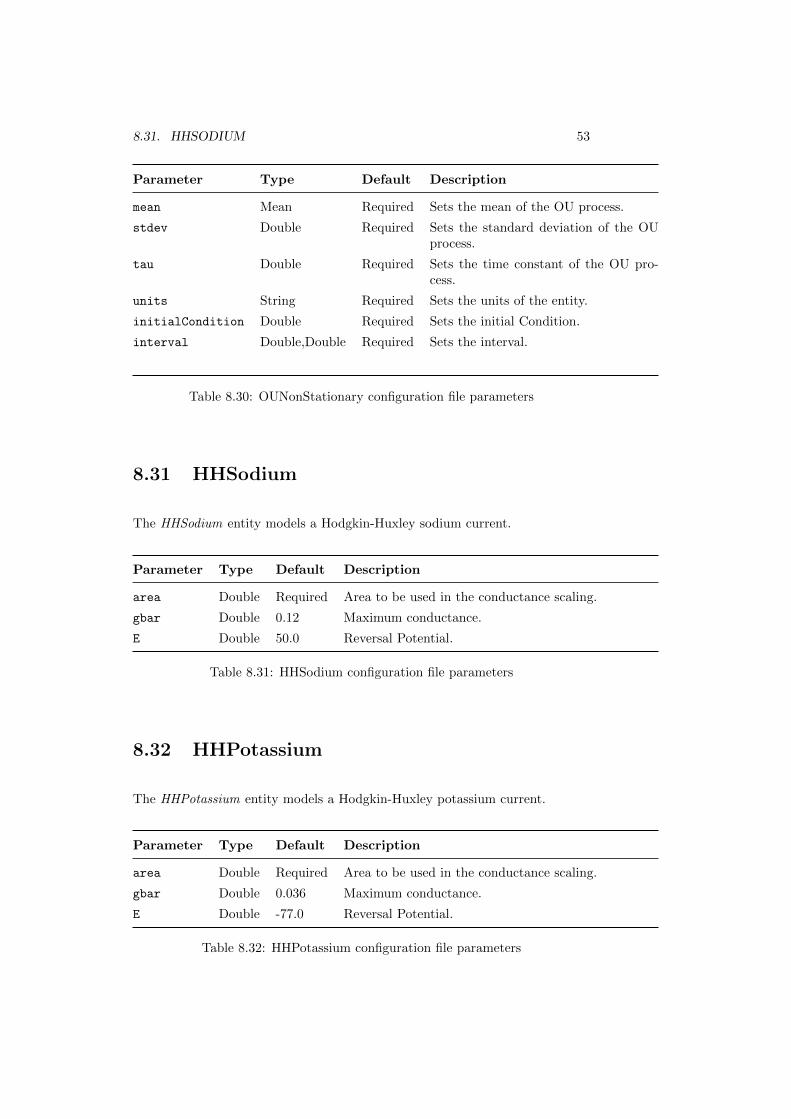
8.31. HHSODIUM 53
Parameter Type Default Description
mean Mean Required Sets the mean of the OU process.
stdev Double Required Sets the standard deviation of the OUprocess.
tau Double Required Sets the time constant of the OU pro-cess.
units String Required Sets the units of the entity.
initialCondition Double Required Sets the initial Condition.
interval Double,Double Required Sets the interval.
Table 8.30: OUNonStationary configuration file parameters
8.31 HHSodium
The HHSodium entity models a Hodgkin-Huxley sodium current.
Parameter Type Default Description
area Double Required Area to be used in the conductance scaling.
gbar Double 0.12 Maximum conductance.
E Double 50.0 Reversal Potential.
Table 8.31: HHSodium configuration file parameters
8.32 HHPotassium
The HHPotassium entity models a Hodgkin-Huxley potassium current.
Parameter Type Default Description
area Double Required Area to be used in the conductance scaling.
gbar Double 0.036 Maximum conductance.
E Double -77.0 Reversal Potential.
Table 8.32: HHPotassium configuration file parameters

54 CHAPTER 8. ENTITIES
8.33 HHSodiumCN
The HHSodiumCN entity models a Hodgkin-Huxley sodium current with Chan-nel Noise.
Parameter Type Default Description
area Double Required Area to be used in the conductance scaling.
gbar Double 0.12 Maximum conductance.
E Double 50.0 Reversal Potential.
gamma Double 10.0 Single channel conductance.
Table 8.33: HHSodiumCN configuration file parameters
8.34 HHPotassiumCN
The HHPotassiumCN entity models a Hodgkin-Huxley potassium current withchannel noise.
Parameter Type Default Description
area Double Required Area to be used in the conductance scaling.
gbar Double 0.036 Maximum conductance.
E Double -77.0 Reversal Potential.
gamma Double 10.0 Single channel conductance.
Table 8.34: HHPotassiumCN configuration file parameters
8.35 HH2Sodium
The HH2Sodium entity models a Hodgkin-Huxley sodium current with temper-ature correction.
Parameter Type Default Description
area Double Required Area to be used in the conductance scaling.
gbar Double 0.12 Maximum conductance.
E Double 50.0 Reversal Potential.
vtraub Double -63 variable to adjust threshold.
temperature Double 36 Reversal Potential.
Table 8.35: HH2Sodium configuration file parameters

8.36. HH2POTASSIUM 55
8.36 HH2Potassium
The HH2Potassium entity models a Hodgkin-Huxley potassium current withtemperature correction.
Parameter Type Default Description
area Double Required Area to be used in the conductance scaling.
gbar Double 0.036 Maximum conductance.
E Double -77.0 Reversal Potential.
vtraub Double -63 variable to adjust threshold.
temperature Double 36 Reversal Potential.
Table 8.36: HH2Potassium configuration file parameters
8.37 MCurrent
The MCurrent entity models a persistent sodium current with temperaturecorrection.
Parameter Type Default Description
area Double Required Area to be used in the conductance scaling.
gbar Double 0.12 Maximum conductance.
E Double 50.0 Reversal Potential.
taumax Double 1000 time constant.
temperature Double 36 Reversal Potential.
Table 8.37: MCurrent configuration file parameters
8.38 WBSodium
The WBSodium entity models a Wang-Buzsaki sodium current.
Parameter Type Default Description
area Double Required Area to be used in the conductance scaling.
gbar Double 0.035 Maximum conductance.
E Double 55.0 Reversal Potential.
Table 8.38: WBSodium configuration file parameters
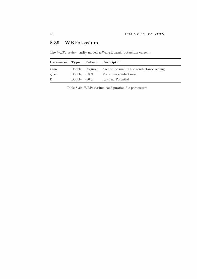
56 CHAPTER 8. ENTITIES
8.39 WBPotassium
The WBPotassium entity models a Wang-Buzsaki potassium current.
Parameter Type Default Description
area Double Required Area to be used in the conductance scaling.
gbar Double 0.009 Maximum conductance.
E Double -90.0 Reversal Potential.
Table 8.39: WBPotassium configuration file parameters

Chapter 9
Additional features
This chapter will describe some additional features present in lcg that mostlikely are not of daily use. However, they can prove rather useful in someparticular scenarios.
9.1 Computation of the SHA checksum
9.2 Adding comments to data files
57

58 CHAPTER 9. ADDITIONAL FEATURES

References
59

60 CHAPTER 9. ADDITIONAL FEATURES

Bibliography
R. Brette, Z. Piwkowska, C. Monier, M. Rudolph-Lilith, J. Fournier, M. Levy,Y. Fregnac, T. Bal, and A. Destexhe, Neuron 59, 379 (2008).
C. Koch and I. Segev, eds., Methods in Neuronal Modeling: From Synapses toNetworks (Computational Neuroscience) (The MIT Press, 1989).
P. Wallisch, Matlab for Neuroscientists, Neuroscience 2011 (Academic Press,2011), ISBN 9780123838360, URL http://books.google.be/books?id=
K3zFygAACAAJ.
Z. F. Mainen and T. J. Sejnowski, Science 268, 1503 (1995).
L. Badel, S. Lefort, R. Brette, C. C. H. Petersen, W. Gerstner, and M. J. E.Richardson, Journal of neurophysiology 99, 656 (2008).
S. Crochet and C. C. H. Petersen, Nature neuroscience 9, 608 (2006).
A. Wallach, D. Eytan, A. Gal, C. Zrenner, and S. Marom, Frontiers in neuro-engineering 4, 3 (2011).
D. Linaro, J. Couto, and M. Giugliano, Journal of Neuroscience Methods 230,5 (2014).
61

62 BIBLIOGRAPHY

Appendix A
MATLAB reference
TODO
63

64 APPENDIX A. MATLAB REFERENCE

Appendix B
UNIX reference
TODO
65