Leachate Characterisation and Assessment of … PDF/2013/January/Salami and...Leachate Characterisation and Assessment of Groundwater Quality: A Case of Soluos Dumpsite in Lagos State,

ISSN: 2354-2373

Leachate Characterisation and

Assessment of Groundwater Quality:

A Case of Soluos Dumpsite in Lagos

State, Nigeria

By

Salami L.

Susu A. A.

Greener Journal of Internet, Information and Communication Systems ISSN: 2354-2373 Vol. 1 (1), pp. 013-032, January 2013.

www.gjournals.org 13

Research Article

Leachate Characterisation and Assessment of Groundwater Quality: A Case of Soluos Dumpsite in

Lagos State, Nigeria

Salami L. and Susu A. A.

Department of Chemical and Polymer Engineering, Lagos State University, Epe, Lagos, Nigeria.

Corresponding Author’s Email: [email protected] ABSTRACT Groundwater contamination due to municipal landfill sites is a threat to ground water integrity. This current research characterised the heavy metals in leachate from Soluos dumpsite in Lagos, Nigeria and assessed the groundwater quality at different distances from the dumpsite for both dry and wet seasons. The contaminants examined are lead, zinc, copper, nickel, chromium, iron, manganese, magnesium, calcium, sodium, potassium and chloride. The results showed that the concentration level of contaminants examined in groundwater samples in all the well investigated fall within the maximum acceptable concentration stipulated by World Health Organisation and National Agency for Food and Drug Administration and Control except for GW2 for wet season; but it will be higher than the level stipulated by the regulatory bodies in future based on the predicted values, hence there is a need to upgrade the dumpsite to prevent future contamination of groundwater. A predictive model for transport of contaminants through a porous medium used in this work predicted the contaminants concentration in groundwater samples near the dumpsite to a very appreciable level of above 93% confidence level, using finite difference method implemented in Matlab 7.0. This showed that the model parameters used which were obtained by sensitivity analysis of previous work of Jhamnani and Singh are suitable for Soluos dumpsite in Lagos State. Descriptive statistics such as mean, variation, standard deviation, standard error and coefficient of variance were used to describe the basic features of the results of groundwater samples. Keywords: Students'use, search engines, information retrieval, web

INTRODUCTION The consumption of available resources has resulted in municipal solid waste (MSW) from industrial to domestic activities, which affect human health. Improper management of solid waste areas has resulted in serious ecological, environmental and health problems. Such practices contribute to widespread environmental pollution as well as spread of diseases (Bakis and Tuncan, 2011). The intensity of man’s activities has led to increasing volume of solid waste worldwide despite the current level of technological advancement and industrialization. Explosive population growth is one major factor responsible for increased municipal solid waste (Longe and Balogun, 2010). The precipitation that falls into a landfill, coupled with any disposed liquid waste, results in the extraction of water-soluble compounds and particulate matter of the waste and the subsequent formation of leachate (salami, 2012). Once leachate is formed and is released to the groundwater environment, it will migrate downward through the unsaturated zone until it eventually reaches the saturated zone. Leachate then will follow the hydraulic gradient of the groundwater system and contaminate the groundwater. Threats to the groundwater from the unlined and uncontrolled landfills exist in many parts of the world, particularly in the under-developed and developing countries (Nigeria inclusive) where the hazardous industrial waste is also co-disposed with municipal waste and no provision to separate secured hazardous landfills exists (Kumar and Alappat, 2003). Even if there are no hazardous wastes placed in municipal landfills, the leachate is still reported as a significant threat to the groundwater (Lema et al., 1988; Lu, 1985). A number of incidences have been reported in the past where leachate had contaminated the surrounding soil and polluted the underlying groundwater aquifer or nearby surface water (Kumar et al., 2002; Kumar and Alappat, 2003; Masters, 1998; Lo, 1996; Chain and Dewalle, 1976; Kelly, 1976; Noble and Arnold, 1991; Qasim and Chiang, 1994; Reinhart and Grosh, 1998; Mc Bean, 1995). The aims and objectives of this work are as follows: (i) to characterise leachate and assess the level of groundwater contamination due to leachate percolation from the unlined Soluos dumpsite in Alimosho Local Government area of Lagos State, Nigeria, (ii) develop suitable model parameters for Soluos dumpsite and



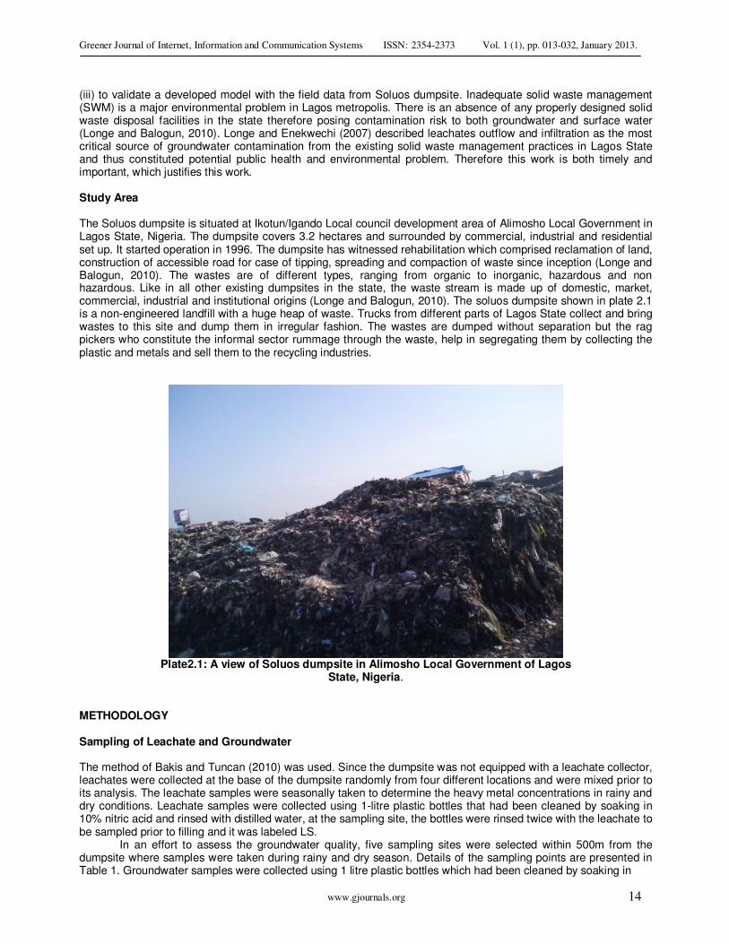
(iii) to validate a developed model with the field data from Soluos dumpsite. Inadequate solid waste management (SWM) is a major environmental problem in Lagos metropolis. There is an absence of any properly designed solid waste disposal facilities in the state therefore posing contamination risk to both groundwater and surface water (Longe and Balogun, 2010). Longe and Enekwechi (2007) described leachates outflow and infiltration as the most critical source of groundwater contamination from the existing solid waste management practices in Lagos State and thus constituted potential public health and environmental problem. Therefore this work is both timely and important, which justifies this work. Study Area The Soluos dumpsite is situated at Ikotun/Igando Local council development area of Alimosho Local Government in Lagos State, Nigeria. The dumpsite covers 3.2 hectares and surrounded by commercial, industrial and residential set up. It started operation in 1996. The dumpsite has witnessed rehabilitation which comprised reclamation of land, construction of accessible road for case of tipping, spreading and compaction of waste since inception (Longe and Balogun, 2010). The wastes are of different types, ranging from organic to inorganic, hazardous and non hazardous. Like in all other existing dumpsites in the state, the waste stream is made up of domestic, market, commercial, industrial and institutional origins (Longe and Balogun, 2010). The soluos dumpsite shown in plate 2.1 is a non-engineered landfill with a huge heap of waste. Trucks from different parts of Lagos State collect and bring wastes to this site and dump them in irregular fashion. The wastes are dumped without separation but the rag pickers who constitute the informal sector rummage through the waste, help in segregating them by collecting the plastic and metals and sell them to the recycling industries.

Plate2.1: A view of Soluos dumpsite in Alimosho Local Government of Lagos

State, Nigeria. METHODOLOGY Sampling of Leachate and Groundwater The method of Bakis and Tuncan (2010) was used. Since the dumpsite was not equipped with a leachate collector, leachates were collected at the base of the dumpsite randomly from four different locations and were mixed prior to its analysis. The leachate samples were seasonally taken to determine the heavy metal concentrations in rainy and dry conditions. Leachate samples were collected using 1-litre plastic bottles that had been cleaned by soaking in 10% nitric acid and rinsed with distilled water, at the sampling site, the bottles were rinsed twice with the leachate to be sampled prior to filling and it was labeled LS.

In an effort to assess the groundwater quality, five sampling sites were selected within 500m from the dumpsite where samples were taken during rainy and dry season. Details of the sampling points are presented in Table 1. Groundwater samples were collected using 1 litre plastic bottles which had been cleaned by soaking in



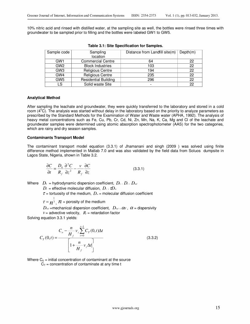
10% nitric acid and rinsed with distilled water, at the sampling site as well, the bottles were rinsed three times with groundwater to be sampled prior to filling and the bottles were labeled GW1 to GW5.

Table 3.1: Site Specification for Samples.

Sample code Sampling location

Distance from Landfill site(m) Depth(m)

GW1 Commercial Centre 64 22 GW2 Block Industries 103 22 GW3 Religious Centre 194 22 GW4 Religious Centre 235 22 GW5 Residential Building 296 22 LS Solid waste Site - 22

Analytical Method After sampling the leachate and groundwater, they were quickly transferred to the laboratory and stored in a cold room (4

0C). The analysis was started without delay in the laboratory based on the priority to analyze parameters as

prescribed by the Standard Methods for the Examination of Water and Waste water (APHA, 1992). The analysis of heavy metal concentrations such as Fe, Cu, Pb, Cr, Cd, Ni, Zn, Mn, Na, K, Ca, Mg and Cl of the leachate and groundwater samples were determined using atomic absorption spectrophotometer (AAS) for the two categories, which are rainy and dry season samples. Contaminants Transport Model The contaminant transport model equation (3.3.1) of Jhamanani and singh (2009 ) was solved using finite difference method implemented in Matlab 7.0 and was also validated by the field data from Soluos dumpsite in Lagos State, Nigeria, shown in Table 3.2.

z

C

R

v

z

C

R

D

t

C

ff

h

∂

∂−

∂

∂=

∂

∂

2

2

(3.3.1)

Where hD = hydrodynamic dispersion coefficient, mdeh DDD +=

eD = effective molecular diffusion, me DD τ=

τ = tortuosity of the medium, mD = molecular diffusion coefficient

n3

1

=τ , n = porosity of the medium

mdD =mechanical dispersion coefficient, vDmd α= , α = dispersivity

v= advective velocity, fR = retardation factor

Solving equation 3.3.1 yields:

∆+

∆−

=

∑−

=

tvH

n

ttCvH

nC

tC

z

f

t

t

Tz

f

o

T

1

),0(

),0(

1

0 (3.3.2)

Where C0 = initial concentration of contaminant at the source CT = concentration of contaminate at any time t



Table 3.3.1: Model parameters for simulation

S/N Model Parameters Unit Value 1 Time yr 50 2 Molecular diffusion coefficient m

2/yr 0.027

3 Mechanical dispersion coefficient m2/yr 0.075

4 Effective molecular diffusion coefficient m2/yr 0.02

5 Dispersivity M 0.15 6 Advective velocity m/yr 0.5 7 Hydrodynamic dispersion m

2/yr 0.095

8 Porosity 0.74

9 Retardation factor 1

10 Equivalent height of leachate M 0.64

11 t∆ S 1

12 z∆ M 1.5

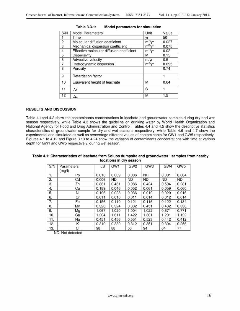
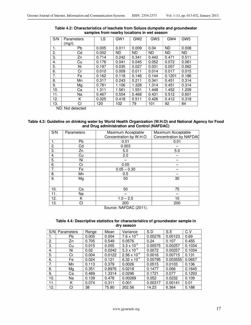
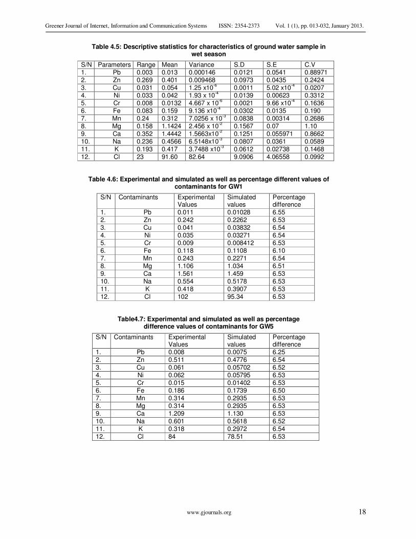
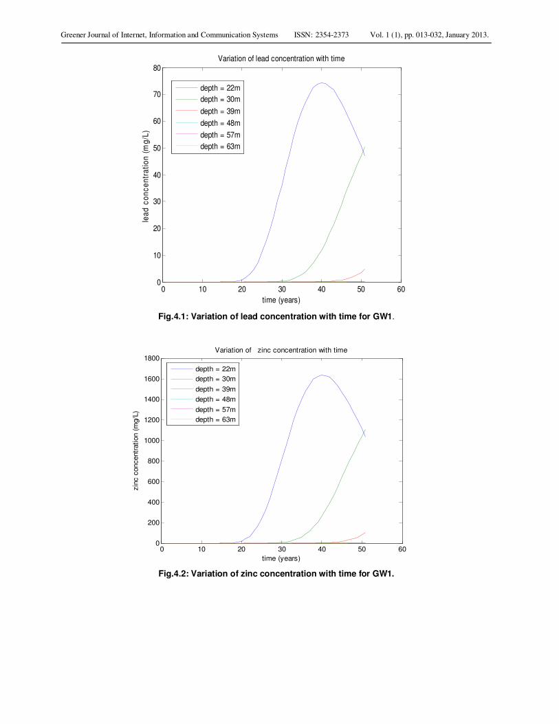
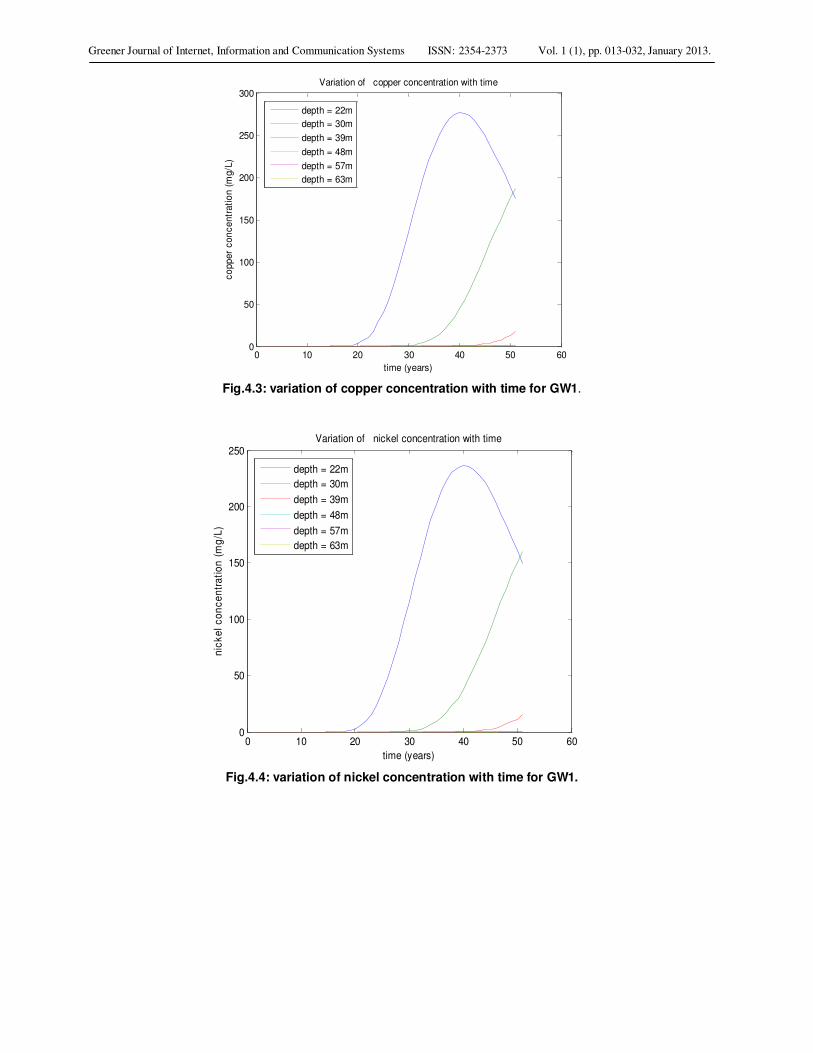
RESULTS AND DISCUSSION Table 4.1and 4.2 show the contaminants concentrations in leachate and groundwater samples during dry and wet season respectively, while Table 4.3 shows the guideline on drinking water by World Health Organization and National Agency for Food and Drug Administration and Control. Tables 4.4 and 4.5 show the descriptive statistics characteristics of groundwater sample for dry and wet seasons respectively, while Table 4.6 and 4.7 show the experimental and simulated as well as percentage different values of contaminants for GW1 and GW5 respectively. Figures 4.1 to 4.12 and Figure 3.13 to 4.24 show the variation of contaminants concentrations with time at various depth for GW1 and GW5 respectively, during wet season.

Table 4.1: Characteristics of leachate from Soluos dumpsite and groundwater samples from nearby locations in dry season

S/N Parameters (mg/l)

LS GW1 GW2 GW3 GW4 GW5

1. Pb 0.010 0.009 0.006 ND 0.001 0.004 2. Cd 0.006 ND ND ND ND ND 3. Zn 0.861 0.461 0.986 0.424 0.594 0.281 4. Cu 0.189 0.046 0.052 0.061 0.059 0.060 5. Ni 0.196 0.028 0.036 0.019 0.020 0.016 6. Cr 0.011 0.010 0.011 0.014 0.012 0.014 7. Fe 0.156 0.110 0.121 0.116 0.122 0.134 8. Mn 0.326 0.324 0.332 0.451 0.432 0.338 9. Mg 1.067 1.020 1.004 1.022 0.671 0.771 10. Ca 1.204 1.611 1.422 1.301 1.201 1.122 11. Na 0.451 0.456 0.551 0.523 0.442 0.412 12. K 0.310 0.330 0.312 0.351 0.304 0.256 13. Cl 98 88 56 94 64 77

ND: Not detected



Table 4.2: Characteristics of leachate from Soluos dumpsite and groundwater

samples from nearby locations in wet season

S/N Parameters (mg/l)

LS GW1 GW2 GW3 GW4 GW5

1. Pb 0.005 0.011 0.009 0.04 ND 0.008 2. Cd 0.002 ND ND ND ND ND 3. Zn 0.714 0.242 0.341 0.442 0.471 0.511 4. Cu 0.176 0.041 0.045 0.052 0.072 0.061 5. Ni 0.197 0.035 0.027 0.031 0.057 0.062 6. Cr 0.010 0.009 0.011 0.014 0.017 0.015 7. Fe 0.162 0.118 0.146 0.144 0.1201 0.186 8. Mn 0.317 0.243 0.211 0.341 0.451 0.314 9. Mg 0.781 1.106 1.328 1.314 0.451 0.314 10. Ca 1.311 1.561 1.551 1.448 1.452 1.209 11. Na 0.467 0.554 0.468 0.431 0.512 0.601 12. K 0.325 0.418 0.511 0.426 0.412 0.318 13. Cl 120 102 79 101 92 84

ND: Not detected Table 4.3: Guideline on drinking water by World Health Organization (W.H.O) and National Agency for Food

and Drug administration and Control (NAFDAC)

S/N Parameters Maximum Acceptable Concentration by W.H.O

Maximum Acceptable Concentration by NAFDAC

1. Pb 0.01 0.01 2. Cd 0.003 – 3. Zn 5.0 5.0 4. Cu 2.0 – 5. Ni – – 6. Cr 0.05 – 7. Fe 0.05 – 0.30 – 8. Mn 0.5 – 9. Mg 50 30

10. Ca 50 75 11. Na – – 12. K 1.0 – 2.0 10 13. Cl 200 200

Source: NAFDAC (2011).

Table 4.4: Descriptive statistics for characteristics of groundwater sample in dry season

S/N Parameters Range Mean Variance S.D S.E C.V 1. Pb 0.005 0.004 7.6 x 10

-6 0.00276 0.00123 0.69

2. Zn 0.705 0.549 0.0576 0.24 0.107 0.455 3. Cu 0.015 0.055 3.3 x 10

-5 0.00575 0.00257 0.1034

4. Ni 0.02 0.0242 5.3 x 10-5

0.0072 0.00257 0.1034 5. Cr 0.004 0.0122 2.56 x 10

-6 0.0016 0.00715 0.131

6. Fe 0.024 0.121 6.32 x 10-5

0.00795 0.003555 0.0657 7. Mn 0.113 0.379 0.0026 0.0515 0.0103 0.136 8. Mg 0.351 0.8976 0.0218 0.1477 0.066 0.1645 9. Ca 0.489 1.3314 0.0296 0.1721 0.077 0.1293 10. Na 0.139 0.478 0.00269 0.052 0.0232 0.109 11. K 0.074 0.311 0.001 0.00317 0.00141 0.01 12. Cl 38 75.80 202.56 14.23 6.364 0.188



Table 4.5: Descriptive statistics for characteristics of ground water sample in

wet season

S/N Parameters Range Mean Variance S.D S.E C.V 1. Pb 0.003 0.013 0.000146 0.0121 0.0541 0.88971 2. Zn 0.269 0.401 0.009468 0.0973 0.0435 0.2424 3. Cu 0.031 0.054 1.25 x10

-6 0.0011 5.02 x10

-4 0.0207

4. Ni 0.033 0.042 1.93 x 10-4

0.0139 0.00623 0.3312 5. Cr 0.008 0.0132 4.667 x 10

-6 0.0021 9.66 x10

-4 0.1636

6. Fe 0.083 0.159 9.136 x10-4

0.0302 0.0135 0.190 7. Mn 0.24 0.312 7.0256 x 10

-3 0.0838 0.00314 0.2686

8. Mg 0.158 1.1424 2.456 x 10-2

0.1567 0.07 1.10 9. Ca 0.352 1.4442 1.5663x10

-2 0.1251 0.055971 0.8662

10. Na 0.236 0.4566 6.5148x10-3

0.0807 0.0361 0.0589 11. K 0.193 0.417 3.7488 x10

-3 0.0612 0.02738 0.1468

12. Cl 23 91.60 82.64 9.0906 4.06558 0.0992

Table 4.6: Experimental and simulated as well as percentage different values of contaminants for GW1

S/N Contaminants Experimental Values

Simulated values

Percentage difference

1. Pb 0.011 0.01028 6.55 2. Zn 0.242 0.2262 6.53 3. Cu 0.041 0.03832 6.54 4. Ni 0.035 0.03271 6.54 5. Cr 0.009 0.008412 6.53 6. Fe 0.118 0.1108 6.10 7. Mn 0.243 0.2271 6.54 8. Mg 1.106 1.034 6.51 9. Ca 1.561 1.459 6.53 10. Na 0.554 0.5178 6.53 11. K 0.418 0.3907 6.53 12. Cl 102 95.34 6.53

Table4.7: Experimental and simulated as well as percentage difference values of contaminants for GW5

S/N Contaminants Experimental Values

Simulated values

Percentage difference

1. Pb 0.008 0.0075 6.25 2. Zn 0.511 0.4776 6.54 3. Cu 0.061 0.05702 6.52 4. Ni 0.062 0.05795 6.53 5. Cr 0.015 0.01402 6.53 6. Fe 0.186 0.1739 6.50 7. Mn 0.314 0.2935 6.53 8. Mg 0.314 0.2935 6.53 9. Ca 1.209 1.130 6.53 10. Na 0.601 0.5618 6.52 11. K 0.318 0.2972 6.54 12. Cl 84 78.51 6.53


Fig.4.1: Variation of lead concentration with time for GW1.

Fig.4.2: Variation of zinc concentration with time for GW1.

0 10 20 30 40 50 600

10

20

30

40

50

60

70

80

time (years)

lea

d c

on

ce

ntr

ati

on

(m

g/L

)

Variation of lead concentration with time

depth = 22m

depth = 30m

depth = 39m

depth = 48m

depth = 57m

depth = 63m

0 10 20 30 40 50 600

200

400

600

800

1000

1200

1400

1600

1800

time (years)

zin

c c

oncentr

ation (

mg/L

)

Variation of zinc concentration with time

depth = 22m

depth = 30m

depth = 39m

depth = 48m

depth = 57m

depth = 63m


Fig.4.3: variation of copper concentration with time for GW1.

Fig.4.4: variation of nickel concentration with time for GW1.

0 10 20 30 40 50 600

50

100

150

200

250

300

time (years)

co

pp

er

co

nc

en

tra

tio

n (

mg

/L)

Variation of copper concentration with time

depth = 22m

depth = 30m

depth = 39m

depth = 48m

depth = 57m

depth = 63m

0 10 20 30 40 50 600

50

100

150

200

250

time (years)

nic

ke

l c

on

ce

ntr

ati

on

(m

g/L

)

Variation of nickel concentration with time

depth = 22m

depth = 30m

depth = 39m

depth = 48m

depth = 57m

depth = 63m


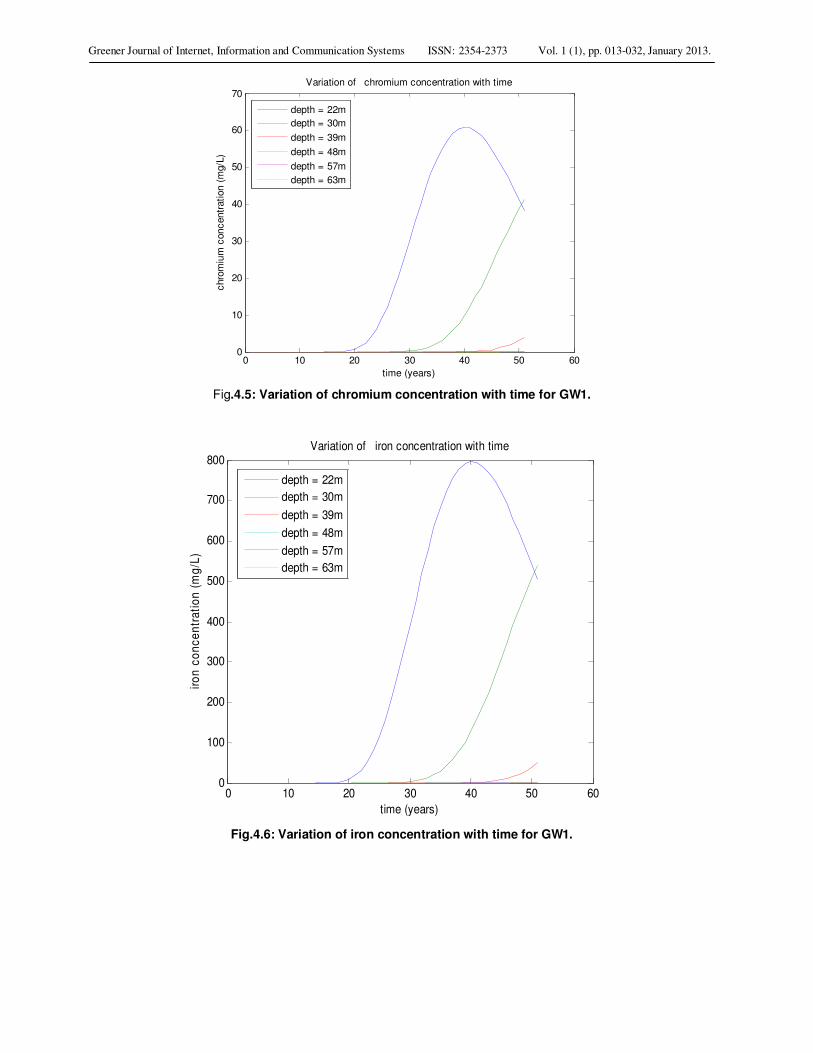
Fig.4.5: Variation of chromium concentration with time for GW1.

Fig.4.6: Variation of iron concentration with time for GW1.

0 10 20 30 40 50 600

10

20

30

40

50

60

70

time (years)

chro

miu

m c

oncentr

ation (

mg/L

)

Variation of chromium concentration with time

depth = 22m

depth = 30m

depth = 39m

depth = 48m

depth = 57m

depth = 63m

0 10 20 30 40 50 600

100

200

300

400

500

600

700

800

time (years)

iro

n c

on

ce

ntr

ati

on

(m

g/L

)

Variation of iron concentration with time

depth = 22m

depth = 30m

depth = 39m

depth = 48m

depth = 57m

depth = 63m


Fig.4.7: Variation of manganese concentration with time for GW1.

Fig.4.8: Variation of magnesium with time for GW1.

0 10 20 30 40 50 600

1000

2000

3000

4000

5000

6000

7000

8000

time (years)

mangnesiu

m c

oncentr

ation (

mg/L

)

Variation of magnesium concentration with time

depth = 22m

depth = 30m

depth = 39m

depth = 48m

depth = 57m

depth = 63m

0 10 20 30 40 50 600

100

200

300

400

500

600

700

800

time (years)

m

agnesiu

m c

oncentr

ation (

mg/L

)


depth = 22m

depth = 30m

depth = 39m

depth = 48m

depth = 57m

depth = 63m


Fig.4.9: Variation of calcium concentration with time for GW1.

Fig.4.10: Variation of sodium concentration with time for GW1.

0 10 20 30 40 50 600

2000

4000

6000

8000

10000

12000

time (years)

ca

lciu

m c

on

ce

ntr

ati

on

(m

g/L

)

Variation of calcium concentration with time

depth = 22m

depth = 30m

depth = 39m

depth = 48m

depth = 57m

depth = 63m

0 10 20 30 40 50 600

500

1000

1500

2000

2500

3000

3500

4000

time (years)

so

diu

m c

on

ce

ntr

ati

on

(m

g/L

)

Variation of sodium concentration with time

depth = 22m

depth = 30m

depth = 39m

depth = 48m

depth = 57m

depth = 63m


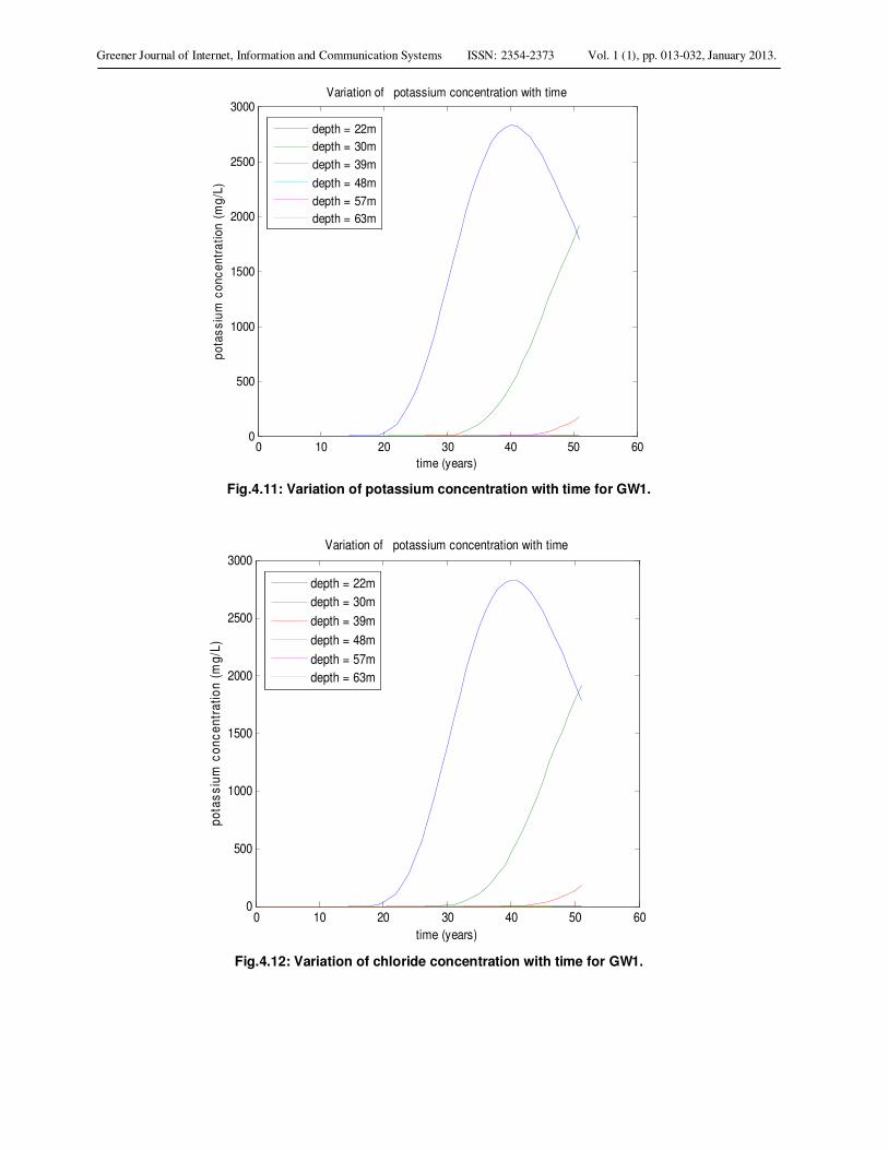
Fig.4.11: Variation of potassium concentration with time for GW1.

Fig.4.12: Variation of chloride concentration with time for GW1.

0 10 20 30 40 50 600

500

1000

1500

2000

2500

3000

time (years)

po

tas

siu

m c

on

ce

ntr

ati

on

(m

g/L

)

Variation of potassium concentration with time

depth = 22m

depth = 30m

depth = 39m

depth = 48m

depth = 57m

depth = 63m

0 10 20 30 40 50 600

500

1000

1500

2000

2500

3000

time (years)

po

tas

siu

m c

on

ce

ntr

ati

on

(m

g/L

)


depth = 22m

depth = 30m

depth = 39m

depth = 48m

depth = 57m

depth = 63m


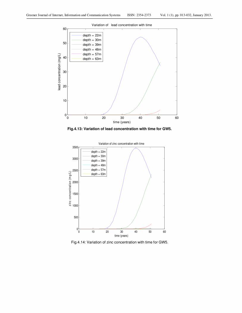
Fig.4.13: Variation of lead concentration with time for GW5.

Fig.4.14: Variation of zinc concentration with time for GW5.

0 10 20 30 40 50 600

10

20

30

40

50

60

time (years)

lead c

oncentr

ation (

mg/L

)

Variation of lead concentration with time

depth = 22m

depth = 30m

depth = 39m

depth = 48m

depth = 57m

depth = 63m

0 10 20 30 40 50 600

500

1000

1500

2000

2500

3000

3500

time (years)

zin

c c

on

ce

ntr

ati

on

(m

g/L

)

Variation of zinc concentration with time

depth = 22m

depth = 30m

depth = 39m

depth = 48m

depth = 57m

depth = 63m


0 10 20 30 40 50 600

20

40

60

80

100

120

time (years)

chro

miu

m c

oncentration (m

g/L

)

Variation of chromium concentration with time

depth = 22m

depth = 30m

depth = 39m

depth = 48m

depth = 57m

depth = 63m

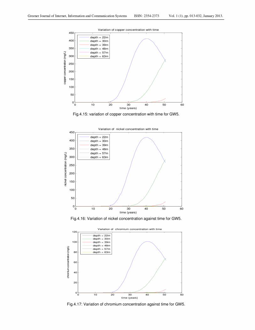
Fig.4.15: variation of copper concentration with time for GW5.

Fig.4.16: Variation of nickel concentration against time for GW5.

Fig.4.17: Variation of chromium concentration against time for GW5.

0 10 20 30 40 50 600

50

100

150

200

250

300

350

400

450

time (years)

copper concentration (m

g/L

)

Variation of copper concentration with time

depth = 22m

depth = 30m

depth = 39m

depth = 48m

depth = 57m

depth = 63m

0 10 20 30 40 50 600

50

100

150

200

250

300

350

400

450

time (years)

nic

kel concentration (m

g/L

)

Variation of nickel concentration with time

depth = 22m

depth = 30m

depth = 39m

depth = 48m

depth = 57m

depth = 63m


Fig.4.18: Variation of iron concentration against time for GW5.

Fig.4.19: Variation of manganese concentration with time for GW5.

0 10 20 30 40 50 600

200

400

600

800

1000

1200

1400

time (years)

iron c

oncentr

ation (

mg/L

)

Variation of iron concentration with time

depth = 22m

depth = 30m

depth = 39m

depth = 48m

depth = 57m

depth = 63m

0 10 20 30 40 50 600

500

1000

1500

2000

2500

time (years)

mag

anes

e c

once

ntr

atio

n (

mg/L

)

Variation of maganese concentration with time

depth = 22m

depth = 30m

depth = 39m

depth = 48m

depth = 57m

depth = 63m


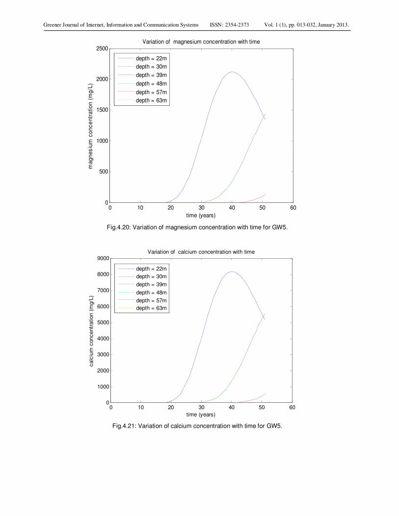
Fig.4.20: Variation of magnesium concentration with time for GW5.

Fig.4.21: Variation of calcium concentration with time for GW5.

0 10 20 30 40 50 600

500

1000

1500

2000

2500

time (years)

ma

gn

es

ium

co

nc

en

tra

tio

n (

mg

/L)


depth = 22m

depth = 30m

depth = 39m

depth = 48m

depth = 57m

depth = 63m

0 10 20 30 40 50 600

1000

2000

3000

4000

5000

6000

7000

8000

9000

time (years)

calc

ium

concentr

ation (

mg/L

)

Variation of calcium concentration with time

depth = 22m

depth = 30m

depth = 39m

depth = 48m

depth = 57m

depth = 63m


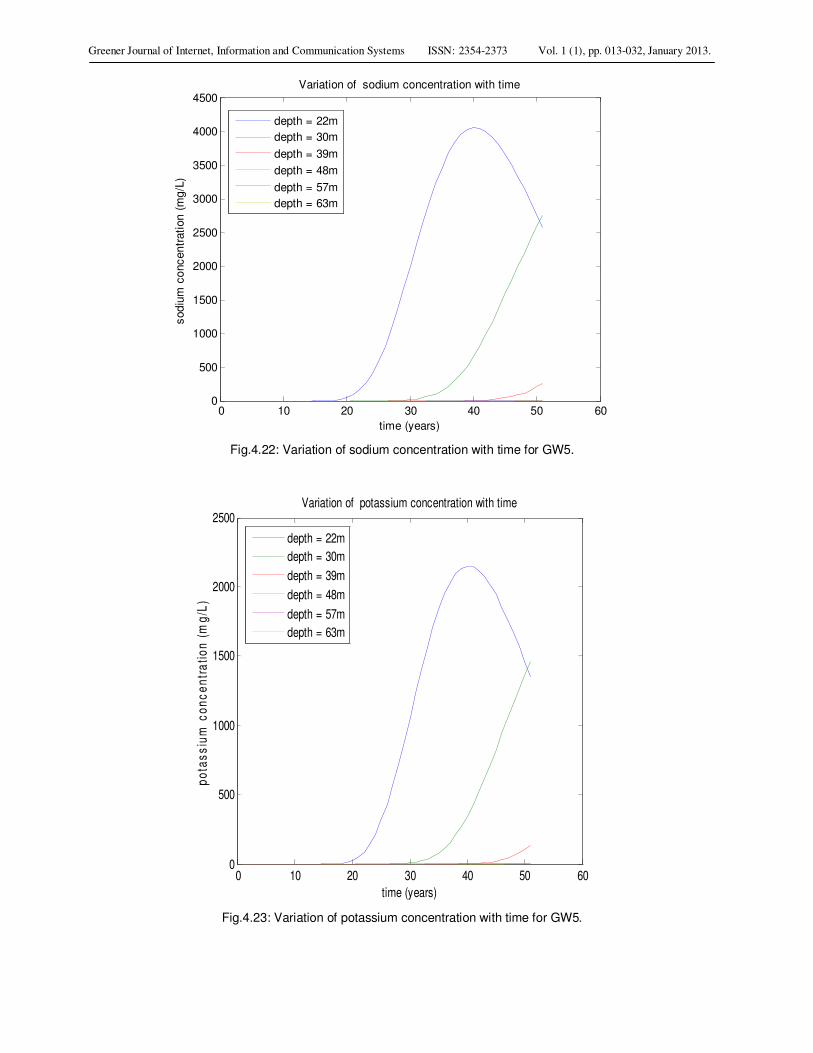
Fig.4.22: Variation of sodium concentration with time for GW5.

Fig.4.23: Variation of potassium concentration with time for GW5.

0 10 20 30 40 50 600

500

1000

1500

2000

2500

3000

3500

4000

4500

time (years)

sod

ium

co

nc

en

trati

on (

mg

/L)

Variation of sodium concentration with time

depth = 22m

depth = 30m

depth = 39m

depth = 48m

depth = 57m

depth = 63m

0 10 20 30 40 50 600

500

1000

1500

2000

2500

time (years)

po

tas

siu

m c

on

ce

ntr

ati

on

(m

g/L

)


depth = 22m

depth = 30m

depth = 39m

depth = 48m

depth = 57m

depth = 63m


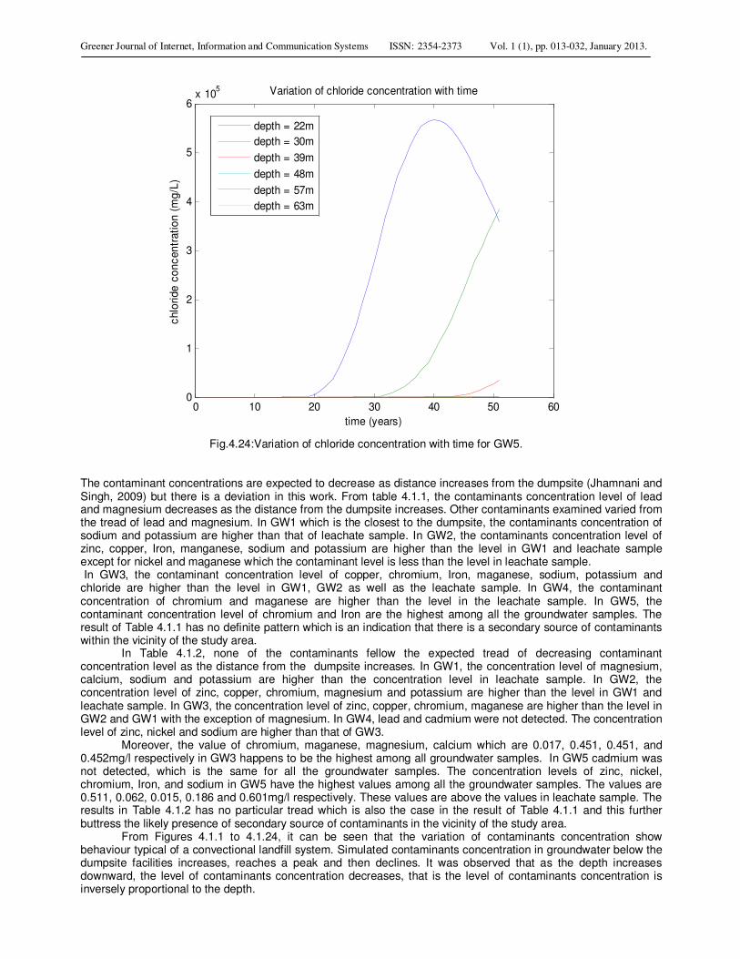
Fig.4.24:Variation of chloride concentration with time for GW5.

The contaminant concentrations are expected to decrease as distance increases from the dumpsite (Jhamnani and Singh, 2009) but there is a deviation in this work. From table 4.1.1, the contaminants concentration level of lead and magnesium decreases as the distance from the dumpsite increases. Other contaminants examined varied from the tread of lead and magnesium. In GW1 which is the closest to the dumpsite, the contaminants concentration of sodium and potassium are higher than that of leachate sample. In GW2, the contaminants concentration level of zinc, copper, Iron, manganese, sodium and potassium are higher than the level in GW1 and leachate sample except for nickel and maganese which the contaminant level is less than the level in leachate sample. In GW3, the contaminant concentration level of copper, chromium, Iron, maganese, sodium, potassium and chloride are higher than the level in GW1, GW2 as well as the leachate sample. In GW4, the contaminant concentration of chromium and maganese are higher than the level in the leachate sample. In GW5, the contaminant concentration level of chromium and Iron are the highest among all the groundwater samples. The result of Table 4.1.1 has no definite pattern which is an indication that there is a secondary source of contaminants within the vicinity of the study area.

In Table 4.1.2, none of the contaminants fellow the expected tread of decreasing contaminant concentration level as the distance from the dumpsite increases. In GW1, the concentration level of magnesium, calcium, sodium and potassium are higher than the concentration level in leachate sample. In GW2, the concentration level of zinc, copper, chromium, magnesium and potassium are higher than the level in GW1 and leachate sample. In GW3, the concentration level of zinc, copper, chromium, maganese are higher than the level in GW2 and GW1 with the exception of magnesium. In GW4, lead and cadmium were not detected. The concentration level of zinc, nickel and sodium are higher than that of GW3.

Moreover, the value of chromium, maganese, magnesium, calcium which are 0.017, 0.451, 0.451, and 0.452mg/l respectively in GW3 happens to be the highest among all groundwater samples. In GW5 cadmium was not detected, which is the same for all the groundwater samples. The concentration levels of zinc, nickel, chromium, Iron, and sodium in GW5 have the highest values among all the groundwater samples. The values are 0.511, 0.062, 0.015, 0.186 and 0.601mg/l respectively. These values are above the values in leachate sample. The results in Table 4.1.2 has no particular tread which is also the case in the result of Table 4.1.1 and this further buttress the likely presence of secondary source of contaminants in the vicinity of the study area.

From Figures 4.1.1 to 4.1.24, it can be seen that the variation of contaminants concentration show behaviour typical of a convectional landfill system. Simulated contaminants concentration in groundwater below the dumpsite facilities increases, reaches a peak and then declines. It was observed that as the depth increases downward, the level of contaminants concentration decreases, that is the level of contaminants concentration is inversely proportional to the depth.

0 10 20 30 40 50 600

1

2

3

4

5

6x 10

5

time (years)

chlo

ride

co

nc

en

trati

on (

mg

/L)

Variation of chloride concentration with time

depth = 22m

depth = 30m

depth = 39m

depth = 48m

depth = 57m

depth = 63m



Though the level of contaminants measured in groundwater samples for both dry and wet season fall within the guideline of National Agency for Food and Drug Administration and Control and World Health Organisation for drinking water, it was obvious from Figures 4.1.1 to 4.1.24 that the concentrations of contaminants in the groundwater around the vicinity of the study area will increase above the level stipulated by the regulatory bodies therefore, there is a need to upgrade the dumpsite.

The soil stratigraphy of Lagos metropolis or the existing sequence of soil type occurring in the metropolis makes land-filling operation very risky, especially when one considers the prevalent high water table in Lagos (Longe and Balogun, 2010). However, the stratigraphy at Soluos dumpsite consisting of clay and silty clay appears to have significantly influenced the moderate level of contaminant found in groundwater samples. The contaminants concentrations for wet season are higher than the contaminants concentrations for dry season which is due to the fact that during wet season, the volume of water available in landfill site for leaching solute from wastes is more than the dry season period. On this basis, the contaminants concentration of wet season were used for simulation of model equation 3.4.1 to predict the level of contaminants in groundwater using finite difference method implemented in Matlab 7.0. The model predicted the experimental results to a very high level of above 93% confidence level as shown in Table 4.1.6 and Table 4.1.7. This revealed that the model parameters of Table 3.4.1 used in this work, which were obtained through sensitivity analysis of the model parameters of Jhamnani and Singh are suitable for Soluos dump site. Descriptive statistics which provides qualitative measure of accuracy about the contaminants such as mean, variance, standard deviation, standard error and coefficient of variance were used to describe the basic features of the field data obtained. In dry season, the mean, variance and standard deviation of contaminants except for chloride range from 0.004 to 1.3314, 2.56 × 10

-6 to 0.0576 and 2.76 × 10

-3 to 0.24 respectively, while the

standard error and coefficient of variance of contaminants except for chloride range from 1.23 x 10-3

to 6.364 and 0.188 to 0.69 respectively. More so, in wet season, the mean, variance and standard deviation of contaminants except for chloride range from 0.0136 to 1.44442, 1.25 × 10

-6 to 2.456 × 10

-2 and 0.00216 to 0.1251 respectively,

while standard error and coefficient of variance of contaminants except for chloride range from 5.02 × 10-4

to 0.0541 and 0.0207 to 0.8897 respectively. CONCLUSION The contaminants concentration is expected to decrease as the distance from the dumpsite increases but the experimental results of this work deviate from such a pattern. The contaminants concentration in groundwater samples in all the well investigated fall within the guideline of maximum acceptable concentration for drinking water by World Health Organization and National Agency for Food and Drug Administration and Control. It was cleared from the predicted results that the level of contaminants concentration in the groundwater in the vicinity of the study area will be above the level stipulated by the regulatory bodies in future. hence there is a need to upgrading the dumpsite to prevent future contamination of groundwater.

The predictive transport model used in this work predicted the experimental results to a very appreciable level of more than 93% confidence level, hence the model parameters used in this work which were obtained through sensitivity analysis of model parameters of Jhamnani and Singh are suitable for Solous dumpsite. Descriptive statistics which provides qualitative measure of accuracy about the samples such as mean, variance, standard deviation, standard error and coefficient of variance were used to describe the basic features of the experimental results. REFERENCES Bakis R and Tuncan A (2011). “An investigation of heavy metal and migration through groundwater from landfill

area of Eskisehir in Turkey”. Environmental Monitoring Assessment. 176: 87 – 98. Chain ESK and DeWalle FB (1976). “Sanitary landfill leachates and their treatment”. ASCE, Journal of

Environmental Engineering Division, 102(2): 411 – 431. Guideline for drinking water (2011). National Agency for Food and Drug Administration and Control. Jhamnani B and Singh SK (2009). Groundwater contamination due to Bhalaswa landfill site in New Dehli.

International Journal of Civil and Environmental Engineering. 1(3):121 – 125. Kelley WE (1976). “Groundwater pollution near a landfill”. ASCE. Journal of Environmental Engineering Division,

102(6): 1189 – 1199. Kumar D and Alappat BJ (2003). “Analysis of leachate contamination potential of a municipal landfill using leachate

pollution index”. Workshop on sustainable landfill management, India, December 3 – 5:147 – 153. Kumar D, Khare M and Alappat BJ (2002). “Threat to groundwater from the municipal landfills in Delhi, India”.

Proceedings of the 28th WEDC Conference on sustainable Environmental Sanitation and Water Services,

Kolkata, India. 377 – 380. Long EO and Balogun MR (2010). “Groundwater quality assessment near a municipal landfill, Lagos. Nigeria”. Research Journal of Applied Science, Engineering and Technology. 2(1):39 – 44.



Longe EO and Enekwechi LO (2007). “Investigation on potential groundwater impacts and influence of local

hydrogeology on natural attenuation of leachate at a municipal landfill”. International Journal of Environmental Science Technology, 4(1): 133 – 140.

LO IMC (1996). “Characteristics and Treatment of Leachates from domestic landfill”. Environmental International, 22(4): 433 – 442.

Lu JCS (1985). “Leachate from municipal landfills, production and management”, Noyes Publisher, Park Ridge. Masters GM (1998). “Introduction to Environmental Engineering and Science”. Prentice – Hall of India Private

Limited, New Delhi, India. Mc Bean EA, Rovers FA and Farquhar GJ (1995). “Solid waste landfill engineering and design”. Prentice Hall, PTR,

Englewood cliff. Noble JJ and Arnold AE (1991). “Experimental and mathematical modeling of moisture transport in landfills”.

Chemical Engineering Communication. 100: 95 – 111. Qasim SR and Chiang W (1994). “Sanitary landfill leachate”. Technomic Publishing Company International, Lan

caster. Reinhart DR and Grosh CJ (1998). “Analysis of Florida MSW landfill leachate quality”. Department of Civil and

Environmental Engineering, University of Central Florida. Salami L (2012). Leachate characterization and assessment of ground water quality: A case of Solous dumpsite in

Lagos State. PhD seminar paper, Lagos State University, Epe, Lagos, Nigeria.

Documents

Leachate Characterisation and Assessment of … PDF/2013/January/Salami and...Leachate Characterisation and Assessment of Groundwater Quality: A Case of Soluos Dumpsite in Lagos State,