Leaf spring modelling

43

Chapter 3

Leaf spring modelling

Accurate full vehicle multi-body simulation models are heavily dependent on the accuracy at

which the subsystems, and more fundamentally, the different components that make up the

subsystems, are modelled. It is needless to say that an accurate model of a leaf spring is

needed if accurate suspension models, and eventually, full vehicle simulation models are to be

created. The leaf spring has been used in vehicle suspensions for many years. It is particularly

popular in commercial vehicles as it is robust, reliable and cost effective. Even though leaf

springs are frequently used in practice they still hold great challenges in creating accurate

mathematical models.

This chapter investigates the modelling of the leaf spring in the spring only configuration as

described in Chapter 2.

1. Introduction

As concluded in Chapter 1, the majority of the leaf spring models in literature considers the

leaf spring configuration where the leaf spring is attached to the vehicle using the fixed-

shackled end configuration, whereas the suspension under investigation in this study has the

leaf spring supported by the hangers, as was shown in Figure 1.4 in Chapter 1. The minimum

requirements set for the leaf spring model are that it has to be able to capture the spring

stiffness and hysteresis loop of the leaf spring. In addition to these requirements, the model

should preferably be able to account for changes in the load length of the leaf spring. It was

shown in Chapter 2 that the stiffness of leaf springs is very sensitive to changes in the loaded

length.

From the literature study conducted in Chapter 1 it was shown that many methods exist that

can be used to model leaf springs with varying success depending on the application. The

methods have different advantages and disadvantages, with some being more computationally

efficient than others. It would be ideal if all the modelling techniques could be evaluated

against each other, comparing accuracy and efficiency. This is however not the goal of this

study, rather a novel leaf spring model will be proposed and compared to one of the modelling

methods from literature namely, neural networks. The aim with the proposed model is not to

add just another modelling method but to try and obtain a model that is able to emulate the

complex behaviour of the multi-leaf spring accurately and still be computationally efficient as

well as being physically meaningful. The proposed elasto-plastic leaf spring model and the

neural network leaf spring model are fundamentally two different techniques. The elasto-

plastic leaf spring model is a physics-based model whereas the neural network model is a non-

physics based model. Physics based models have certain advantages over non-physics based

models. The main advantage of a physics based model, especially in the context of this study,

is that the model has parameters that are associated with certain aspects of the behaviour of

C h a p t e r 3 Lea f S p r i n g M o d e l l i n g

44

the system. This makes it possible to use the physics based model in situations where the

parameters can be optimized as well as performing sensitivity analysis. On the other hand the

non-physics based neural network model has the potential to have a better computational

efficiency than the other leaf spring models including the elasto-plastic leaf spring model.

This computational efficiency can be utilized in the situations mentioned above by using the

neural network in a gray-box or semi-physical approach as mentioned in Dreyfus (2005). The

physics based and non-physics based models each have their advantages and therefore both

are investigated in this chapter. The elasto-plastic leaf spring model will be presented first

after which the neural network approach to modelling the leaf spring will be discussed.

2. Elasto-plastic leaf spring model

Some of the physical phenomena that gives multi-leaf springs their unique characteristics are

the contact and friction processes that are present between the individual blades. These

processes are responsible for the hysteretic behaviour of the leaf spring. The contact and

friction processes are complex phenomena and modelling them are computationally

expensive. Additional complexity is added to the contact and friction process as adjacent

blades may have varying pressure distributions between them (Li and Li, 2004 and Omar et

al., 2004). This paragraph presents the elasto-plastic leaf spring model that is able to emulate

the nonlinear, hysteretic behaviour of a leaf spring without needing to explicitly model the

complex microscopic physical phenomena such as contact and friction. The elasto-plastic leaf

spring model will first be used to model the multi-leaf spring. After the feasibility of the

elasto-plastic leaf spring model has been determined it will then be applied to the parabolic

leaf spring.

The following paragraph serves as an introduction to the elasto-plastic leaf spring model by

stating the origin of the idea for the model.

2.1. The behaviour of materials and leaf springs

Comparing the force-displacement characteristics of the multi-leaf spring to the stress-strain

behaviour of engineering materials, several similarities can be observed of which the most

notable is the two stiffness regimes that are present (see Figure 3.1). Figure 3.1(a) shows the

stress-strain curve for the elastic, linear hardening material model. From this curve two

stiffness regimes can clearly be observed. Regime 1 coincides with the elastic deformation of

the material and regime 2 with plastic deformation. Figure 3.1(b) presents a typical force-

displacement characteristic of a multi-leaf spring. On the force-displacement characteristic

two stiffness regimes can also be observed. Figure 3.1(c) shows the stress-strain curve of

materials and the force-displacement characteristic of a multi leaf spring superimposed. From

this figure it is concluded that it might be possible to use models, similar to material models,

to emulate the behaviour of multi-leaf springs. This led to the investigation of developing a

leaf spring model that was based on the approach used to model material behaviour.

Understanding the behaviour of engineering materials, and multi-leaf springs, requires that the

microscopic mechanisms be considered. A brief summary of the deformation behaviour of

materials and the models used to describe them will be given in the following paragraph. The

similarities between the microscopic mechanisms involved in materials and in leaf springs

will also be noted before presenting the elasto-plastic leaf spring models.

L e a f S p r i n g M o d e l l i n g C h a p t e r 3

45

Figure 3.1. Similarities between the behaviour of leaf springs and engineering materials. (a) Stress-strain curve

of elastic, linear-hardening material model. (b) Multi-leaf spring force-displacement characteristic. (c)

Superposition of force-displacement characteristic of a multi-leaf spring and the stress-strain curve of the elastic,

linear-hardening material model.

2.1.1. Deformation behaviour and models of materials

Materials may experience two kinds of deformation: elastic and inelastic (plastic or creep).

Elastic deformation is non-permanent and is associated with the stretching, but not breaking,

of inter-atomic bonds. In contrast, the two types of inelastic deformation involve processes

where bonds with original atom neighbours are broken and new bonds are formed with the

new neighbours as large numbers of atoms or molecules move relative to one another. If the

inelastic deformation is time dependent, it is classed as creep, as distinguished from plastic

deformation, which is not time dependent. The mechanism of plastic deformation is different

for crystalline and non-crystalline (amorphous) materials. For crystalline solids, deformation

is accomplished by means of a process called slip, which involves the motion of dislocations.

Whereas, plastic deformation in non-crystalline solids occur by a viscous flow mechanism.

Refer to Callister (2003) and Dowling (1999) for a more detailed discussion.

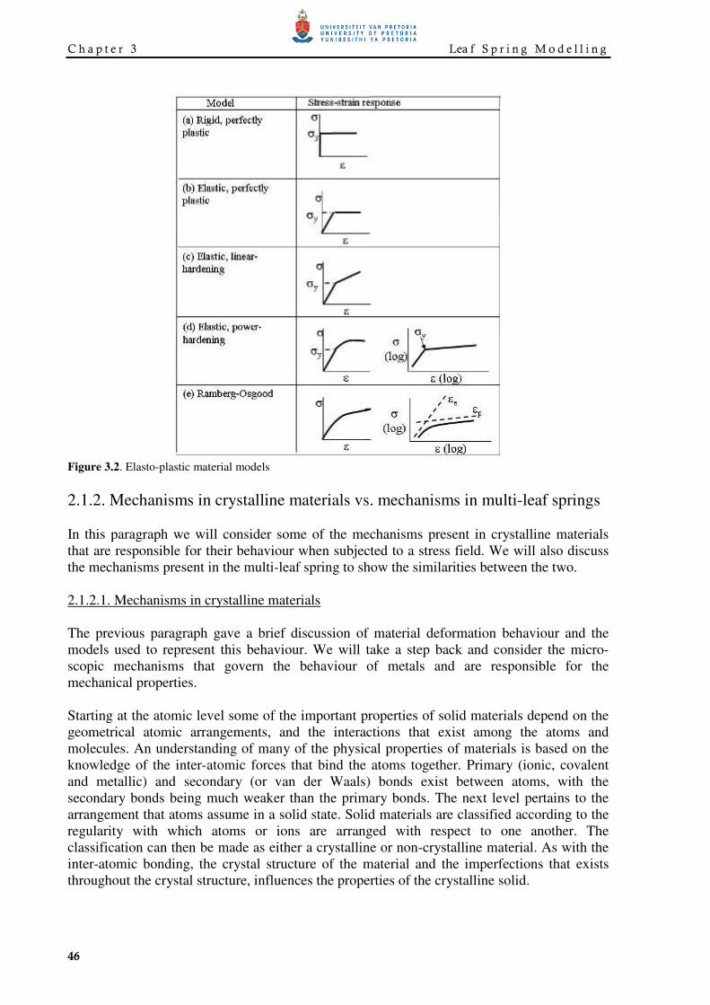
Several models that exist to describe the deformation behaviour of materials are shown in

Figure 3.2. This figure shows the elasto-plastic stress-strain curves of the models subjected to

a monotonic loading. All the curves have an elastic portion until the material starts yielding

after which the stress and strains are no longer linearly proportional i.e. does not follow

Hooke’s law. This region is associated with plastic deformation.


46

Figure 3.2. Elasto-plastic material models

2.1.2. Mechanisms in crystalline materials vs. mechanisms in multi-leaf springs

In this paragraph we will consider some of the mechanisms present in crystalline materials

that are responsible for their behaviour when subjected to a stress field. We will also discuss

the mechanisms present in the multi-leaf spring to show the similarities between the two.

2.1.2.1. Mechanisms in crystalline materials

The previous paragraph gave a brief discussion of material deformation behaviour and the

models used to represent this behaviour. We will take a step back and consider the micro-

scopic mechanisms that govern the behaviour of metals and are responsible for the

mechanical properties.

Starting at the atomic level some of the important properties of solid materials depend on the

geometrical atomic arrangements, and the interactions that exist among the atoms and

molecules. An understanding of many of the physical properties of materials is based on the

knowledge of the inter-atomic forces that bind the atoms together. Primary (ionic, covalent

and metallic) and secondary (or van der Waals) bonds exist between atoms, with the

secondary bonds being much weaker than the primary bonds. The next level pertains to the

arrangement that atoms assume in a solid state. Solid materials are classified according to the

regularity with which atoms or ions are arranged with respect to one another. The

classification can then be made as either a crystalline or non-crystalline material. As with the

inter-atomic bonding, the crystal structure of the material and the imperfections that exists

throughout the crystal structure, influences the properties of the crystalline solid.


47

It was mentioned in paragraph 2.1.1 that elastic deformation is associated with the stretching,

but not breaking, of inter-atomic bonds. Whereas, plastic deformation on a microscopic scale

corresponds to the net movement of large numbers of atoms in response to an applied stress

(Callister, 2003). During this process, inter-atomic bonds must be broken and then reformed.

In crystalline solids, plastic deformation most often involves the motion of dislocations (linear

imperfections in the atomic structure). Callister (2003) discusses the characteristics of

dislocations and their involvement in plastic deformation in more detail. Only some of the

basic concepts will be discussed here.

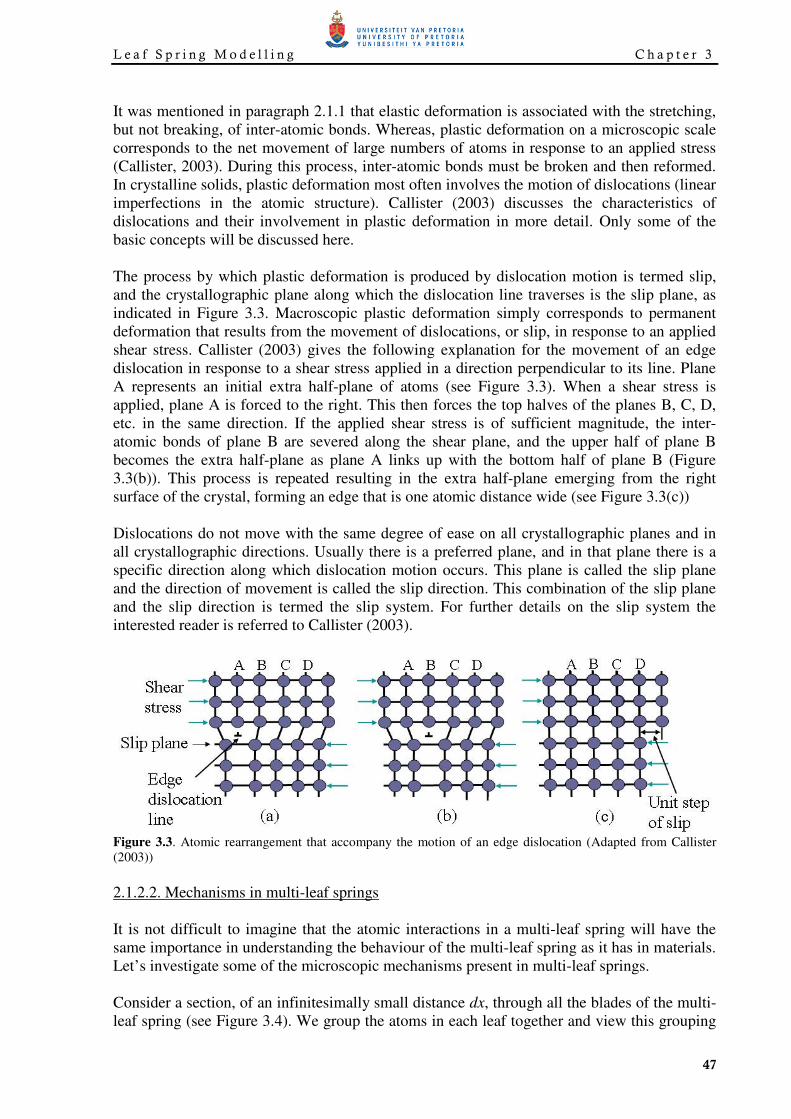
The process by which plastic deformation is produced by dislocation motion is termed slip,

and the crystallographic plane along which the dislocation line traverses is the slip plane, as

indicated in Figure 3.3. Macroscopic plastic deformation simply corresponds to permanent

deformation that results from the movement of dislocations, or slip, in response to an applied

shear stress. Callister (2003) gives the following explanation for the movement of an edge

dislocation in response to a shear stress applied in a direction perpendicular to its line. Plane

A represents an initial extra half-plane of atoms (see Figure 3.3). When a shear stress is

applied, plane A is forced to the right. This then forces the top halves of the planes B, C, D,

etc. in the same direction. If the applied shear stress is of sufficient magnitude, the inter-

atomic bonds of plane B are severed along the shear plane, and the upper half of plane B

becomes the extra half-plane as plane A links up with the bottom half of plane B (Figure

3.3(b)). This process is repeated resulting in the extra half-plane emerging from the right

surface of the crystal, forming an edge that is one atomic distance wide (see Figure 3.3(c))

Dislocations do not move with the same degree of ease on all crystallographic planes and in

all crystallographic directions. Usually there is a preferred plane, and in that plane there is a

specific direction along which dislocation motion occurs. This plane is called the slip plane

and the direction of movement is called the slip direction. This combination of the slip plane

and the slip direction is termed the slip system. For further details on the slip system the

interested reader is referred to Callister (2003).

Figure 3.3. Atomic rearrangement that accompany the motion of an edge dislocation (Adapted from Callister

(2003))

2.1.2.2. Mechanisms in multi-leaf springs

It is not difficult to imagine that the atomic interactions in a multi-leaf spring will have the

same importance in understanding the behaviour of the multi-leaf spring as it has in materials.

Let’s investigate some of the microscopic mechanisms present in multi-leaf springs.

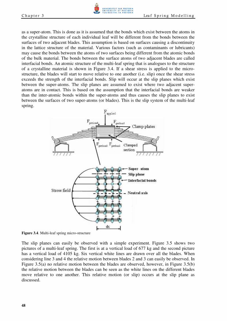
Consider a section, of an infinitesimally small distance dx, through all the blades of the multi-

leaf spring (see Figure 3.4). We group the atoms in each leaf together and view this grouping


48

as a super-atom. This is done as it is assumed that the bonds which exist between the atoms in

the crystalline structure of each individual leaf will be different from the bonds between the

surfaces of two adjacent blades. This assumption is based on surfaces causing a discontinuity

in the lattice structure of the material. Various factors (such as contaminants or lubricants)

may cause the bonds between the atoms of two surfaces being different from the atomic bonds

of the bulk material. The bonds between the surface atoms of two adjacent blades are called

interfacial bonds. An atomic structure of the multi-leaf spring that is analogues to the structure

of a crystalline material is shown in Figure 3.4. If a shear stress is applied to the micro-

structure, the blades will start to move relative to one another (i.e. slip) once the shear stress

exceeds the strength of the interfacial bonds. Slip will occur at the slip planes which exist

between the super-atoms. The slip planes are assumed to exist where two adjacent super-

atoms are in contact. This is based on the assumption that the interfacial bonds are weaker

than the inter-atomic bonds within the super-atoms and thus causes the slip planes to exist

between the surfaces of two super-atoms (or blades). This is the slip system of the multi-leaf

spring.

Figure 3.4. Multi-leaf spring micro-structure

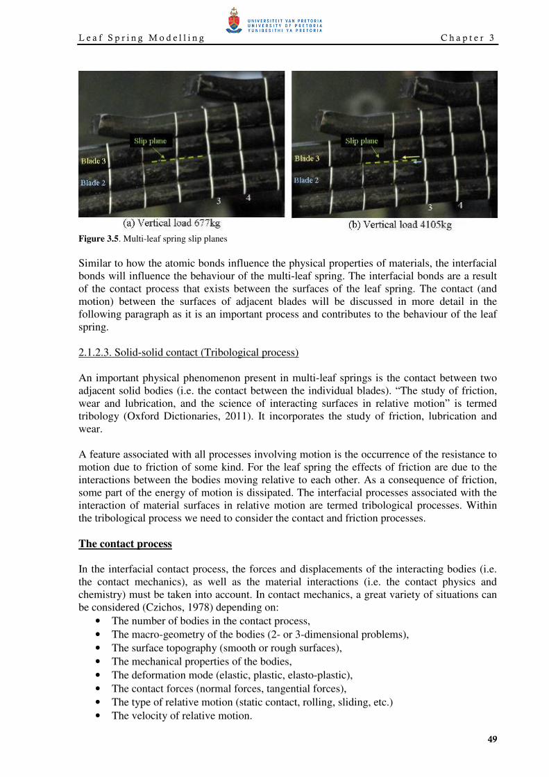
The slip planes can easily be observed with a simple experiment. Figure 3.5 shows two

pictures of a multi-leaf spring. The first is at a vertical load of 677 kg and the second picture

has a vertical load of 4105 kg. Six vertical white lines are drawn over all the blades. When

considering line 3 and 4 the relative motion between blades 2 and 3 can easily be observed. In

Figure 3.5(a) no relative motion between the blades are observed, however, in Figure 3.5(b)

the relative motion between the blades can be seen as the white lines on the different blades

move relative to one another. This relative motion (or slip) occurs at the slip plane as

discussed.


49

Figure 3.5. Multi-leaf spring slip planes

Similar to how the atomic bonds influence the physical properties of materials, the interfacial

bonds will influence the behaviour of the multi-leaf spring. The interfacial bonds are a result

of the contact process that exists between the surfaces of the leaf spring. The contact (and

motion) between the surfaces of adjacent blades will be discussed in more detail in the

following paragraph as it is an important process and contributes to the behaviour of the leaf

spring.

2.1.2.3. Solid-solid contact (Tribological process)

An important physical phenomenon present in multi-leaf springs is the contact between two

adjacent solid bodies (i.e. the contact between the individual blades). “The study of friction,

wear and lubrication, and the science of interacting surfaces in relative motion” is termed

tribology (Oxford Dictionaries, 2011). It incorporates the study of friction, lubrication and

wear.

A feature associated with all processes involving motion is the occurrence of the resistance to

motion due to friction of some kind. For the leaf spring the effects of friction are due to the

interactions between the bodies moving relative to each other. As a consequence of friction,

some part of the energy of motion is dissipated. The interfacial processes associated with the

interaction of material surfaces in relative motion are termed tribological processes. Within

the tribological process we need to consider the contact and friction processes.

The contact process

In the interfacial contact process, the forces and displacements of the interacting bodies (i.e.

the contact mechanics), as well as the material interactions (i.e. the contact physics and

chemistry) must be taken into account. In contact mechanics, a great variety of situations can

be considered (Czichos, 1978) depending on:

• The number of bodies in the contact process,

• The macro-geometry of the bodies (2- or 3-dimensional problems),

• The surface topography (smooth or rough surfaces),

• The mechanical properties of the bodies,

• The deformation mode (elastic, plastic, elasto-plastic),

• The contact forces (normal forces, tangential forces),

• The type of relative motion (static contact, rolling, sliding, etc.)

• The velocity of relative motion.


50

Czichos (1978) gives reference to review articles on various aspects of contact mechanics.

Some of the aspects with which the contact physics and chemistry are concerned with are the

interfacial bonding and the generation of adhesive junctions.

The friction process

Whenever two solid bodies are in direct or indirect contact and made to slide relative to one

another, there is always a resistance to the motion. This resistance to the motion is called

friction and is energy consuming. Friction has long been the interest of many scientific studies

and includes work done by Galileo, da Vinci, Amontons and Coulomb.

Different models have been developed in order to describe the macroscopic friction force

between two sliding surfaces. Czichos (1978) state that based on the existing knowledge of

the topography and the composition of solid surfaces, the following microscopic view of

sliding friction is postulated: friction occurs through asperity (surface atom) interactions. In

this model the macroscopic friction force can be expressed as the sum of microscopic friction

forces at the individual micro-contacts. The energy dissipated can be calculated in a similar

manner. The main processes involved in the different stages of the formation and separation

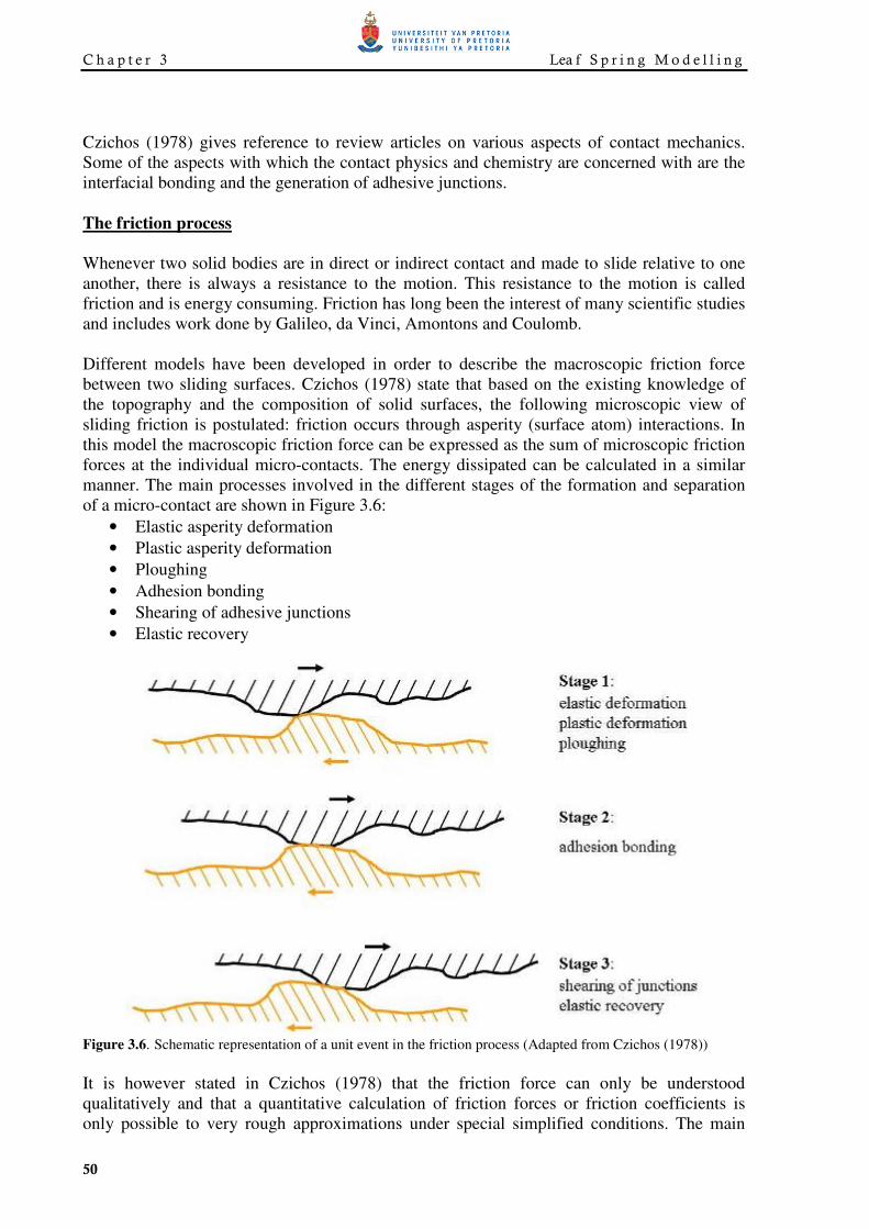
of a micro-contact are shown in Figure 3.6:

• Elastic asperity deformation

• Plastic asperity deformation

• Ploughing

• Adhesion bonding

• Shearing of adhesive junctions

• Elastic recovery

Figure 3.6. Schematic representation of a unit event in the friction process (Adapted from Czichos (1978))

It is however stated in Czichos (1978) that the friction force can only be understood

qualitatively and that a quantitative calculation of friction forces or friction coefficients is

only possible to very rough approximations under special simplified conditions. The main


51

reason for this is due to the incomplete knowledge of the surface properties of solids. In

another study, Merkle and Marks (2007) describe the friction between crystalline bodies using

a model that unifies elements of dislocation drag, contact mechanics and interface theory.

Their model, as yet, is not able to explain all the frictional effects, but is able to give

reasonable results for both the dynamic and static frictional coefficients.

2.1.2.4. Conclusion

From the brief discussion above, it was shown that there exist similarities between the

mechanisms governing the behaviour of engineering materials and multi-leaf springs. It is

clear that the mechanisms involved and the tribological processes associated with the multi-

leaf spring are complex. Therefore, instead of trying to model it on a microscopic level we

will rather try and quantify it on a macroscopic level. In material science, instead of modelling

the inter-atomic bonds, dislocation, etc., the material is characterised on a macroscopic level

by obtaining its mechanical properties. Similarly, the multi-leaf spring will be characterized

on a macroscopic level by obtaining its mechanical properties.

2.2. Mechanical properties of a multi-leaf spring

From the mechanisms governing the behaviour of multi-leaf springs as discussed above, it is

postulated that the multi-leaf spring will have two different stiffness regimes. In the study

conducted by Hoyle (2004) the presence of two stiffness regimes were noted. He associated

the first stiffness regime with small suspension deflections, which was significantly stiffer

than the second stiffness regime, which was associated with larger suspension deflections.

Hoyle (2004) attributed this to the fact that “if a certain load has to be applied to the

suspension in order to overcome the friction between the blades, then until this load has been

reached the blades will act like a solid beam. Implicit in this scenario is the possibility that for

small deflections the locked blades will have a different, and probably higher, stiffness than

the sum of the stiffnesses of the individual blades”. His suspicions are correct; the two

stiffness regimes are due to the characteristic of the friction process that governs the

characteristic of the interfacial bonds. Upon loading or unloading of the spring, the friction

force will cause the individual blades to have no relative motion (i.e. no slip). As the load is

increased (in the case of loading) or decreased (in the case of unloading) the friction force will

reach a critical point at which point the individual blades will start to move relative to one

another (i.e. slip along the slip planes). This causes the multi-leaf spring to act as either a solid

beam (no slip between blades) or a layered beam (slip between blades).

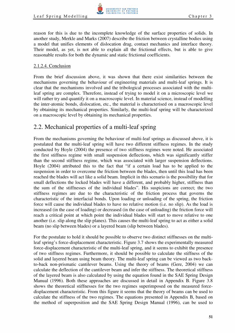
For the postulate to hold it should be possible to observe two distinct stiffnesses on the multi-

leaf spring’s force-displacement characteristic. Figure 3.7 shows the experimentally measured

force-displacement characteristic of the multi-leaf spring, and it seems to exhibit the presence

of two stiffness regimes. Furthermore, it should be possible to calculate the stiffness of the

solid and layered beam using beam theory. The multi-leaf spring can be viewed as two back-

to-back non-prismatic cantilever beams. Using the theory of beams (Gere, 2004) we can

calculate the deflection of the cantilever beam and infer the stiffness. The theoretical stiffness

of the layered beam is also calculated by using the equation found in the SAE Spring Design

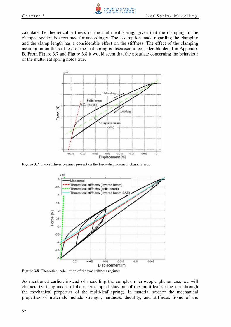
Manual (1996). Both these approaches are discussed in detail in Appendix B. Figure 3.8

shows the theoretical stiffnesses for the two regimes superimposed on the measured force-

displacement characteristic. From this figure it seems that the theory of beams can be used to

calculate the stiffness of the two regimes. The equations presented in Appendix B, based on

the method of superposition and the SAE Spring Design Manual (1996), can be used to


52

calculate the theoretical stiffness of the multi-leaf spring, given that the clamping in the

clamped section is accounted for accordingly. The assumption made regarding the clamping

and the clamp length has a considerable effect on the stiffness. The effect of the clamping

assumption on the stiffness of the leaf spring is discussed in considerable detail in Appendix

B. From Figure 3.7 and Figure 3.8 it would seem that the postulate concerning the behaviour

of the multi-leaf spring holds true.

Figure 3.7. Two stiffness regimes present on the force-displacement characteristic

Figure 3.8. Theoretical calculation of the two stiffness regimes

As mentioned earlier, instead of modelling the complex microscopic phenomena, we will

characterize it by means of the macroscopic behaviour of the multi-leaf spring (i.e. through

the mechanical properties of the multi-leaf spring). In material science the mechanical

properties of materials include strength, hardness, ductility, and stiffness. Some of the


53

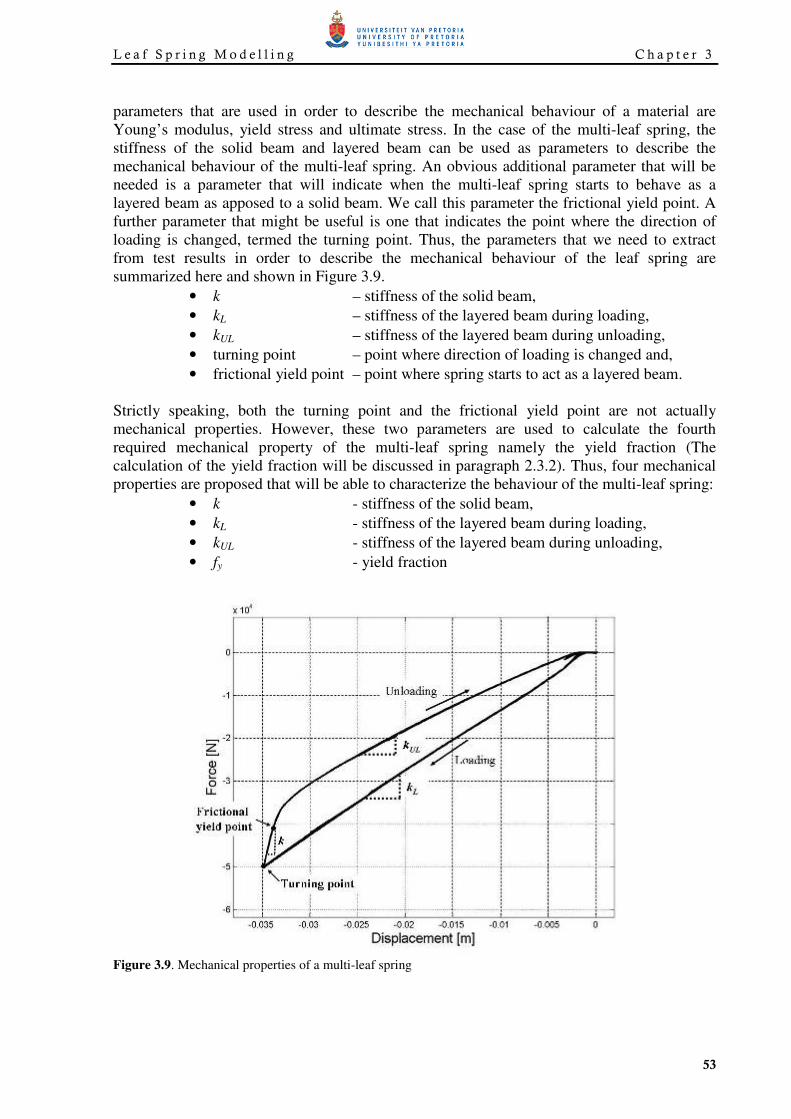
parameters that are used in order to describe the mechanical behaviour of a material are

Young’s modulus, yield stress and ultimate stress. In the case of the multi-leaf spring, the

stiffness of the solid beam and layered beam can be used as parameters to describe the

mechanical behaviour of the multi-leaf spring. An obvious additional parameter that will be

needed is a parameter that will indicate when the multi-leaf spring starts to behave as a

layered beam as apposed to a solid beam. We call this parameter the frictional yield point. A

further parameter that might be useful is one that indicates the point where the direction of

loading is changed, termed the turning point. Thus, the parameters that we need to extract

from test results in order to describe the mechanical behaviour of the leaf spring are

summarized here and shown in Figure 3.9.

• k – stiffness of the solid beam,

• kL – stiffness of the layered beam during loading,

• kUL – stiffness of the layered beam during unloading,

• turning point – point where direction of loading is changed and,

• frictional yield point – point where spring starts to act as a layered beam.

Strictly speaking, both the turning point and the frictional yield point are not actually

mechanical properties. However, these two parameters are used to calculate the fourth

required mechanical property of the multi-leaf spring namely the yield fraction (The

calculation of the yield fraction will be discussed in paragraph 2.3.2). Thus, four mechanical

properties are proposed that will be able to characterize the behaviour of the multi-leaf spring:

• k - stiffness of the solid beam,

• kL - stiffness of the layered beam during loading,

• kUL - stiffness of the layered beam during unloading,

• fy - yield fraction

Figure 3.9. Mechanical properties of a multi-leaf spring


54

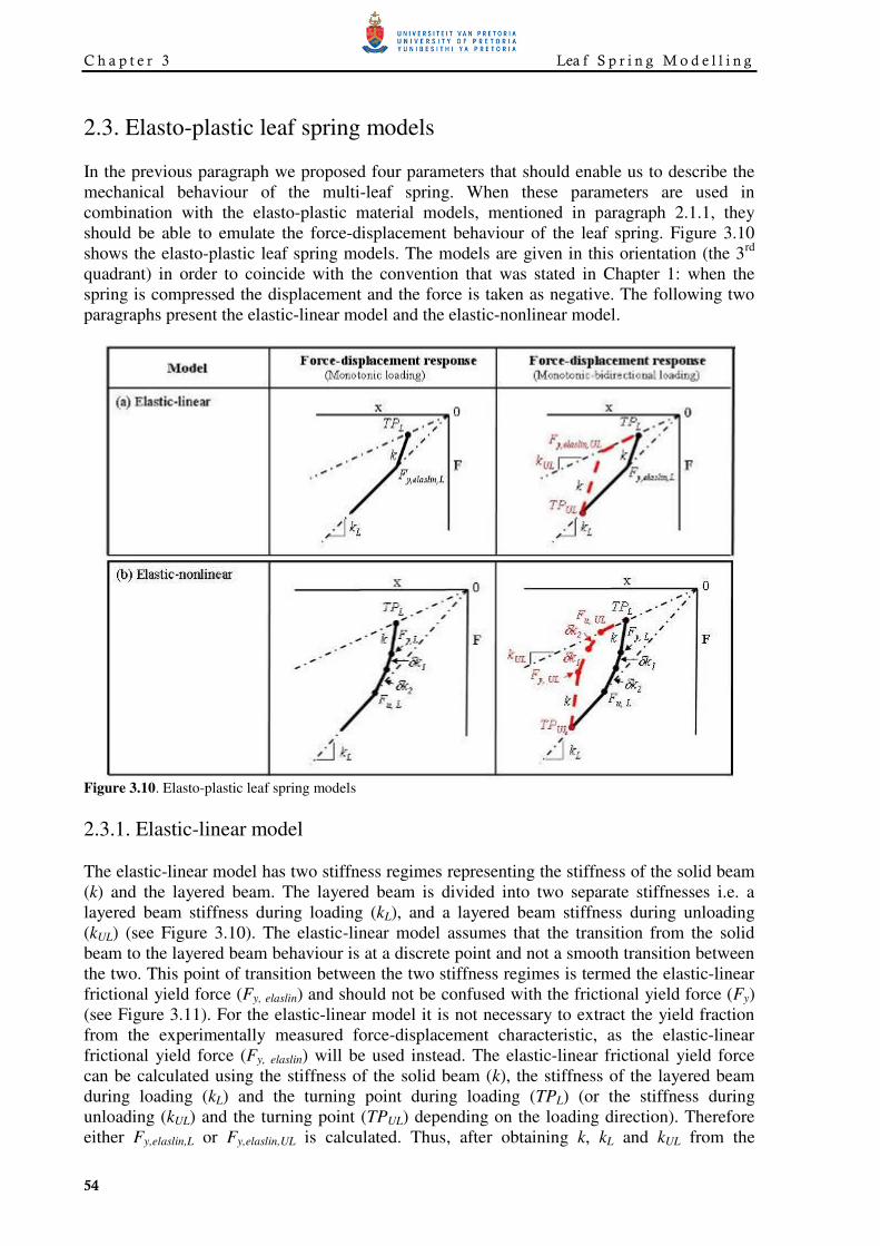
2.3. Elasto-plastic leaf spring models

In the previous paragraph we proposed four parameters that should enable us to describe the

mechanical behaviour of the multi-leaf spring. When these parameters are used in

combination with the elasto-plastic material models, mentioned in paragraph 2.1.1, they

should be able to emulate the force-displacement behaviour of the leaf spring. Figure 3.10

shows the elasto-plastic leaf spring models. The models are given in this orientation (the 3rd

quadrant) in order to coincide with the convention that was stated in Chapter 1: when the

spring is compressed the displacement and the force is taken as negative. The following two

paragraphs present the elastic-linear model and the elastic-nonlinear model.

Figure 3.10. Elasto-plastic leaf spring models

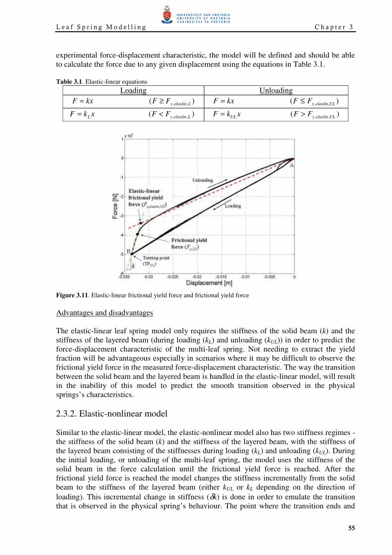
2.3.1. Elastic-linear model

The elastic-linear model has two stiffness regimes representing the stiffness of the solid beam

(k) and the layered beam. The layered beam is divided into two separate stiffnesses i.e. a

layered beam stiffness during loading (kL), and a layered beam stiffness during unloading

(kUL) (see Figure 3.10). The elastic-linear model assumes that the transition from the solid

beam to the layered beam behaviour is at a discrete point and not a smooth transition between

the two. This point of transition between the two stiffness regimes is termed the elastic-linear

frictional yield force (Fy, elaslin) and should not be confused with the frictional yield force (Fy)

(see Figure 3.11). For the elastic-linear model it is not necessary to extract the yield fraction

from the experimentally measured force-displacement characteristic, as the elastic-linear

frictional yield force (Fy, elaslin) will be used instead. The elastic-linear frictional yield force

can be calculated using the stiffness of the solid beam (k), the stiffness of the layered beam

during loading (kL) and the turning point during loading (TPL) (or the stiffness during

unloading (kUL) and the turning point (TPUL) depending on the loading direction). Therefore

either Fy,elaslin,L or Fy,elaslin,UL is calculated. Thus, after obtaining k, kL and kUL from the


55

experimental force-displacement characteristic, the model will be defined and should be able

to calculate the force due to any given displacement using the equations in Table 3.1.

Table 3.1. Elastic-linear equations

Loading Unloading

kxF = )( ,, LelaslinyFF ≥ kxF = )( ,, ULelaslinyFF ≤

xkF L= )( ,, LelaslinyFF < xkF UL= )( ,, ULelaslinyFF >

Figure 3.11. Elastic-linear frictional yield force and frictional yield force

Advantages and disadvantages

The elastic-linear leaf spring model only requires the stiffness of the solid beam (k) and the

stiffness of the layered beam (during loading (kL) and unloading (kUL)) in order to predict the

force-displacement characteristic of the multi-leaf spring. Not needing to extract the yield

fraction will be advantageous especially in scenarios where it may be difficult to observe the

frictional yield force in the measured force-displacement characteristic. The way the transition

between the solid beam and the layered beam is handled in the elastic-linear model, will result

in the inability of this model to predict the smooth transition observed in the physical

springs’s characteristics.

2.3.2. Elastic-nonlinear model

Similar to the elastic-linear model, the elastic-nonlinear model also has two stiffness regimes -

the stiffness of the solid beam (k) and the stiffness of the layered beam, with the stiffness of

the layered beam consisting of the stiffnesses during loading (kL) and unloading (kUL). During

the initial loading, or unloading of the multi-leaf spring, the model uses the stiffness of the

solid beam in the force calculation until the frictional yield force is reached. After the

frictional yield force is reached the model changes the stiffness incrementally from the solid

beam to the stiffness of the layered beam (either kUL or kL depending on the direction of

loading). This incremental change in stiffness (δk) is done in order to emulate the transition

that is observed in the physical spring’s behaviour. The point where the transition ends and


56

the spring again behaves as a layered beam is called the ultimate frictional yield force (Fu).

Beyond the ultimate frictional yield force the stiffness of the layered beam is used.

In addition to the parameters k, kUL and kL that we needed to extract from the measured force-

displacement characteristic for the elastic-linear model, we need to get the yield fraction for

the elastic-nonlinear model. The yield fraction is calculated from the frictional yield force and

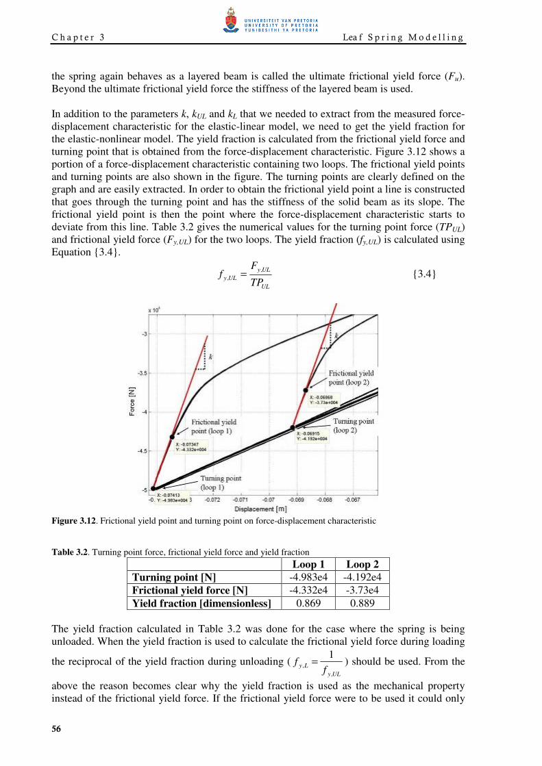
turning point that is obtained from the force-displacement characteristic. Figure 3.12 shows a

portion of a force-displacement characteristic containing two loops. The frictional yield points

and turning points are also shown in the figure. The turning points are clearly defined on the

graph and are easily extracted. In order to obtain the frictional yield point a line is constructed

that goes through the turning point and has the stiffness of the solid beam as its slope. The

frictional yield point is then the point where the force-displacement characteristic starts to

deviate from this line. Table 3.2 gives the numerical values for the turning point force (TPUL)

and frictional yield force (Fy,UL) for the two loops. The yield fraction (fy,UL) is calculated using

Equation {3.4}.

UL

ULy

ULyTP

Ff

,

, = {3.4}

Figure 3.12. Frictional yield point and turning point on force-displacement characteristic

Table 3.2. Turning point force, frictional yield force and yield fraction

Loop 1 Loop 2

Turning point [N] -4.983e4 -4.192e4

Frictional yield force [N] -4.332e4 -3.73e4

Yield fraction [dimensionless] 0.869 0.889

The yield fraction calculated in Table 3.2 was done for the case where the spring is being

unloaded. When the yield fraction is used to calculate the frictional yield force during loading

the reciprocal of the yield fraction during unloading (ULy

Lyf

f,

,

1= ) should be used. From the

above the reason becomes clear why the yield fraction is used as the mechanical property

instead of the frictional yield force. If the frictional yield force were to be used it could only


57

be applied to a single loop, whereas the yield fraction can be applied to all loops. Once the

mechanical properties (k, kUL, kL and the yield fraction) have been obtained, the equations in

Table 3.3 can be used to calculate the force for any given displacement.

Table 3.3. Elastic-nonlinear equations

Loading Unloading

Solid beam kxF = )( ,LyFF ≥ kxF = )( ,ULyFF ≤

Transition kxF δ= ( LyFF ,<

AND LuFF ,≥ )

kxF δ= ( ULyFF ,>

AND ULuFF ,≤ )

Layered beam xkF L= ( LuFF ,< ) xkF UL= ( ULuFF ,> )

Advantages and disadvantages

The elastic-nonlinear leaf spring model will be able to give better predictions for the transition

from the solid beam to the layered beam behaviour. However, there might be cases where it is

difficult to obtain the frictional yield point from the force-displacement characteristic, and

will therefore make it difficult to calculate the yield fraction. Furthermore, it has not yet been

proven that the yield fraction will not change between loops and therefore it may occur that

the yield fraction cannot be calculated in certain scenarios. Under these conditions the elastic-

nonlinear model will not be able to accurately represent the transient behaviour.

2.4. Validation of the elasto-plastic leaf spring model

The proposed elasto-plastic leaf spring models will now be implemented and validated against

measured data. The experimental data obtained using the spring only setup presented in

paragraph 2.1.2 in Chapter 2 will be used. The data from the spring only setup is used as this

setups isolates the leaf spring and does not include effects from other components.

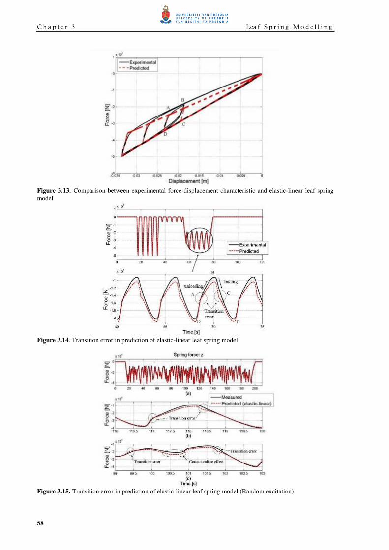
2.4.1. Elastic-linear model

The predictions of the elastic-linear model and the measured data, subjected to the same

displacement input, are compared in Figure 3.13 and Figure 3.14. Figure 3.13 shows the

comparison of the force-displacement characteristic and Figure 3.14 shows the comparison of

the spring force. The spring force was measured by the load cell situated between the actuator

and the multi-leaf spring (see Figure 2.16 in Chapter 2). From both figures the error this

model makes in predicting the transition between the solid and layered beam behaviour, can

clearly be observed. It can also be observed that there is a deviation in the amplitude at the

point at which the loading direction is changed (points B and D). Additionally, the model and

the physical system were subjected to a random displacement input. Figure 3.15 shows the

comparison of the spring force. The transitional error is shown in Figure 3.15(b). The errors

that the model makes in the transitional phase are compounded in cycles that have small

amplitudes. This compounding effect is shown in Figure 3.15(c). All the comparisons indicate

that the elastic-linear model gives good predictions of the vertical behaviour of the leaf spring.


58

Figure 3.13. Comparison between experimental force-displacement characteristic and elastic-linear leaf spring

model

Figure 3.14. Transition error in prediction of elastic-linear leaf spring model

Figure 3.15. Transition error in prediction of elastic-linear leaf spring model (Random excitation)


59

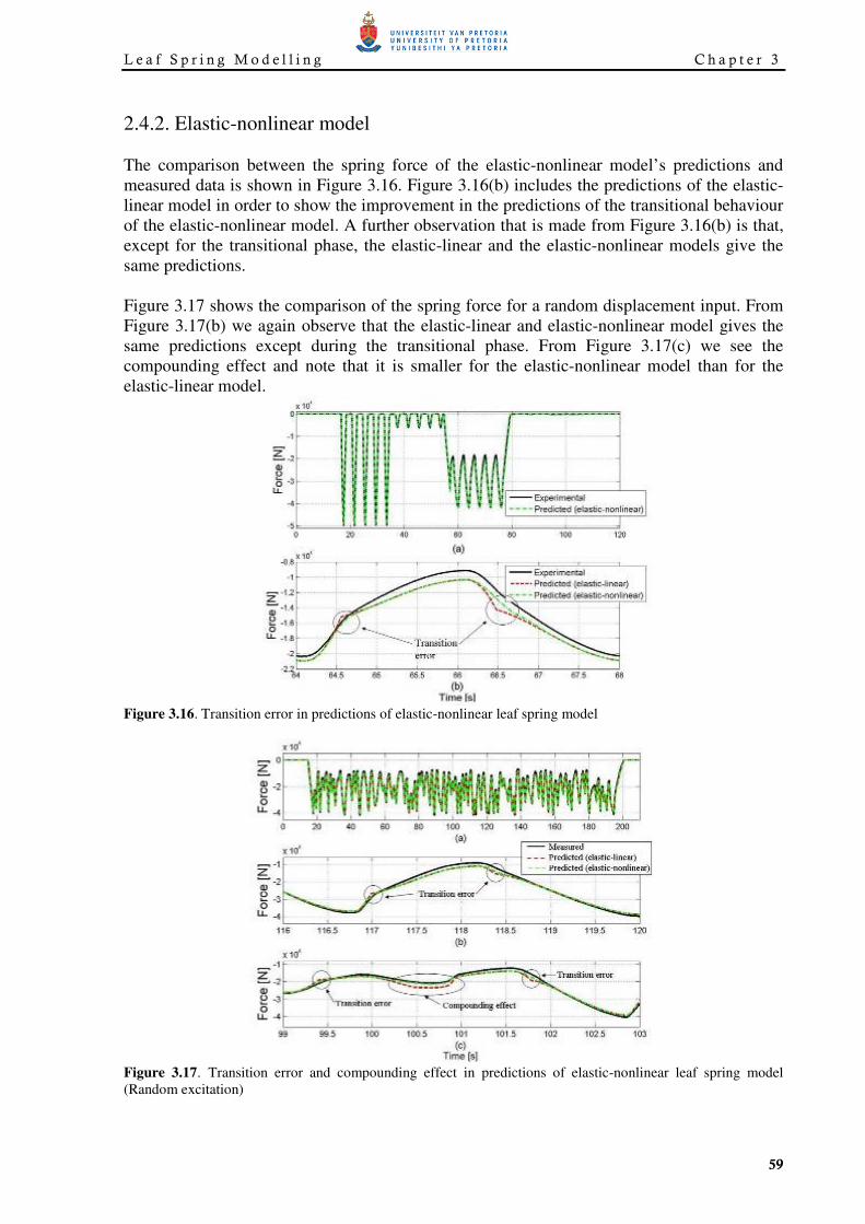
2.4.2. Elastic-nonlinear model

The comparison between the spring force of the elastic-nonlinear model’s predictions and

measured data is shown in Figure 3.16. Figure 3.16(b) includes the predictions of the elastic-

linear model in order to show the improvement in the predictions of the transitional behaviour

of the elastic-nonlinear model. A further observation that is made from Figure 3.16(b) is that,

except for the transitional phase, the elastic-linear and the elastic-nonlinear models give the

same predictions.

Figure 3.17 shows the comparison of the spring force for a random displacement input. From

Figure 3.17(b) we again observe that the elastic-linear and elastic-nonlinear model gives the

same predictions except during the transitional phase. From Figure 3.17(c) we see the

compounding effect and note that it is smaller for the elastic-nonlinear model than for the

elastic-linear model.

Figure 3.16. Transition error in predictions of elastic-nonlinear leaf spring model

Figure 3.17. Transition error and compounding effect in predictions of elastic-nonlinear leaf spring model

(Random excitation)


60

2.5. Conclusion

The proposed leaf-spring model is based on material behaviour and material models. The

analogy implies that the leaf-spring should have two stiffness regimes that are associated with

the no-slip and slip conditions, which corresponds to the elastic and inelastic deformation of

engineering materials. It was shown that the leaf-spring does indeed have these two stiffness

regimes present in its behaviour and that they can be estimated accurately by using beam

theory.

The comparisons between the predictions of the elastic-linear and the elastic-nonlinear model,

with the measured data, correlate well. Compared to the predictions of the elastic-linear model

the elastic-nonlinear model gives better predictions especially during the transitional phase.

The results show that the mechanical properties of the leaf spring, used with the elasto-plastic

leaf spring models, are able to predict the behaviour of the leaf spring for both sinusoidal and

random displacement inputs. From the qualitative results it can be concluded that the elasto-

plastic leaf spring models can accurately predict the complex behaviour of the multi-leaf

spring without needing to model the complex microscopic mechanisms. The elasto-plastic

leaf spring model offers a simple and efficient mathematical representation of the multi-leaf

spring, requiring only three parameters (when using the elastic-linear formulation) to

accurately capture the behaviour of the multi-leaf spring.

3. Elasto-plastic leaf spring model applied to the parabolic leaf

spring

In this paragraph the novel elasto-plastic leaf spring (EPLS) model, presented in the previous

paragraph and used to model a multi-leaf spring, will now be applied to a parabolic leaf

spring.

Figure 3.18 shows the force-displacement characteristic of the multi-leaf spring and the

parabolic leaf spring that was obtained using the spring only setup. The difference in the two

leaf spring’s characteristics can be observed. The parabolic leaf spring has a much smaller

hysteresis loop. This is due to the parabolic leaf spring having fewer blades and contact

between blades only at the ends which implies that there is less friction. The elastic-linear

formulation of the EPLS model, presented in paragraph 2.3.1, will be used to simulate the

parabolic leaf spring. The elastic-linear model is used as the parabolic leaf spring has a more

rapid transition between the solid and layered beam behaviour. This makes it difficult to

extract the yield fraction required by the elastic-nonlinear model. Furthermore, because the

transition from the solid beam to the layered beam behaviour takes place so rapidly the error

the elastic-linear model will make in the area of transition is much smaller than when used to

model the multi-leaf spring. Figure 3.19 shows the error the elastic-linear model will make

when used to model the multi-leaf spring and the parabolic leaf spring.


61

Figure 3.18. Force-displacement characteristic multi-leaf spring and parabolic leaf spring

Figure 3.19. Transition error of using linear-elastic model on multi-leaf spring and parabolic leaf spring

3.1. Extracting mechanical properties for the elastic-linear parabolic leaf spring

model

The parameters we need to extract from the experimental characteristic of the parabolic leaf

spring in order to define the elastic-linear model are: the stiffness of the solid beam (k) and the

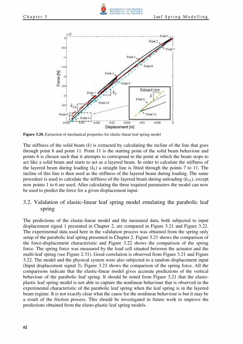
stiffness of the layered beam during loading (kL) and unloading (kUL). Figure 3.20 indicates

the extraction of the three parameters from the experimental characteristic of the parabolic

leaf spring. The force-displacement characteristic shown in Figure 3.20 was obtained using

the spring only setup discussed in paragraph 3.1.2 in Chapter 2.


62

Figure 3.20. Extraction of mechanical properties for elastic-linear leaf spring model

The stiffness of the solid beam (k) is extracted by calculating the incline of the line that goes

through point 6 and point 11. Point 11 is the starting point of the solid beam behaviour and

points 6 is chosen such that it attempts to correspond to the point at which the beam stops to

act like a solid beam and starts to act as a layered beam. In order to calculate the stiffness of

the layered beam during loading (kL) a straight line is fitted through the points 7 to 11. The

incline of this line is then used as the stiffness of the layered beam during loading. The same

procedure is used to calculate the stiffness of the layered beam during unloading (kUL), except

now points 1 to 6 are used. After calculating the three required parameters the model can now

be used to predict the force for a given displacement input.

3.2. Validation of elastic-linear leaf spring model emulating the parabolic leaf

spring

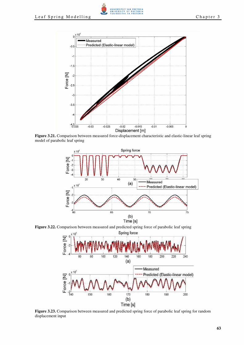
The predictions of the elastic-linear model and the measured data, both subjected to input

displacement signal 1 presented in Chapter 2, are compared in Figure 3.21 and Figure 3.22.

The experimental data used here in the validation process was obtained from the spring only

setup of the parabolic leaf spring presented in Chapter 2. Figure 3.21 shows the comparison of

the force-displacement characteristic and Figure 3.22 shows the comparison of the spring

force. The spring force was measured by the load cell situated between the actuator and the

multi-leaf spring (see Figure 2.31). Good correlation is observed from Figure 3.21 and Figure

3.22. The model and the physical system were also subjected to a random displacement input

(Input displacement signal 3). Figure 3.23 shows the comparison of the spring force. All the

comparisons indicate that the elastic-linear model gives accurate predictions of the vertical

behaviour of the parabolic leaf spring. It should be noted from Figure 3.21 that the elasto-

plastic leaf spring model is not able to capture the nonlinear behaviour that is observed in the

experimental characteristic of the parabolic leaf spring when the leaf spring is in the layered

beam regime. It is not exactly clear what the cause for the nonlinear behaviour is but it may be

a result of the friction process. This should be investigated in future work to improve the

predictions obtained from the elasto-plastic leaf spring models.


63

Figure 3.21. Comparison between measured force-displacement characteristic and elastic-linear leaf spring

model of parabolic leaf spring

Figure 3.22. Comparison between measured and predicted spring force of parabolic leaf spring

Figure 3.23. Comparison between measured and predicted spring force of parabolic leaf spring for random

displacement input


64

3.3. Conclusion

The elastic-linear formulation of the EPLS model was used to emulate the parabolic leaf

spring. After the required mechanical properties of the parabolic leaf spring were extracted, in

order to parameterise the elastic-linear leaf spring model, the model was simulated. The result

from the elastic-linear leaf spring model was compared to the measured data for which good

correlation was obtained.

4. Loaded length changes of a simply supported leaf spring

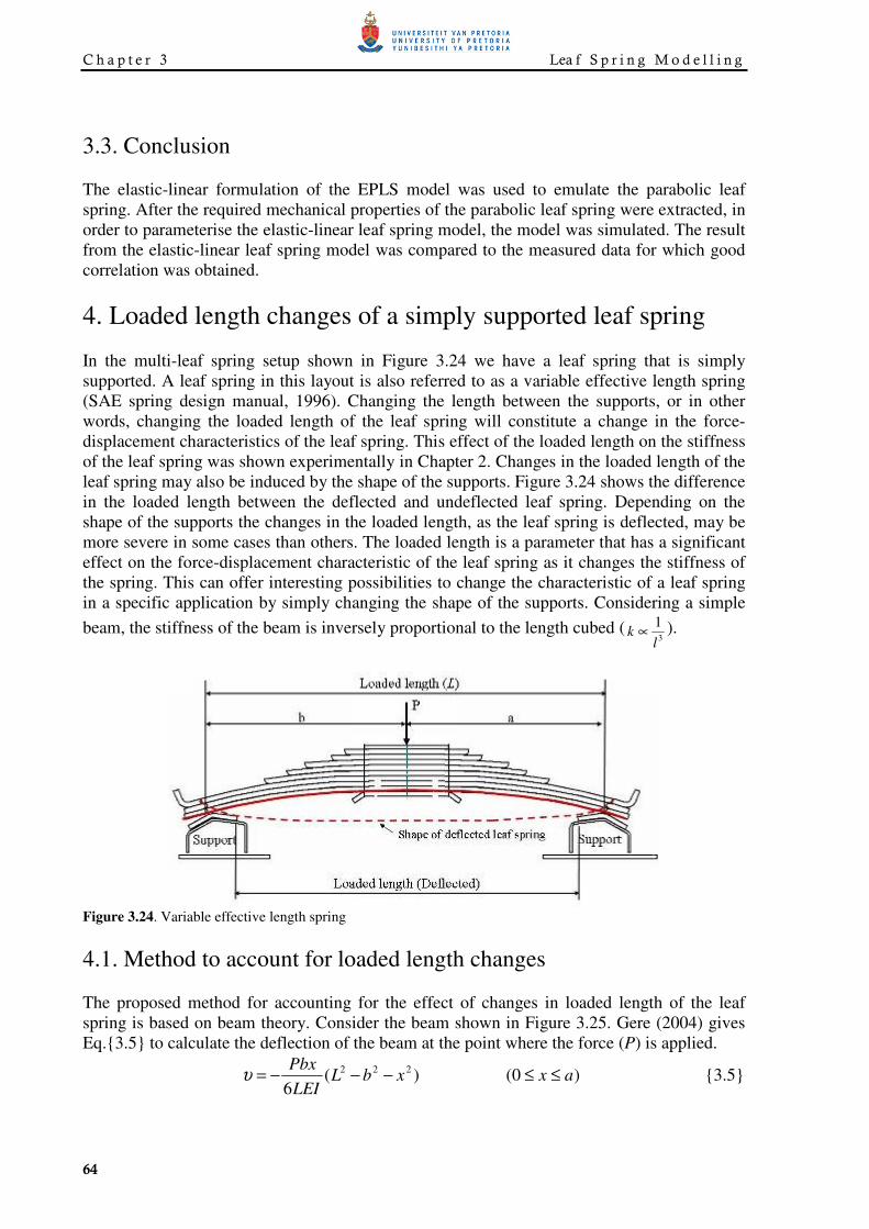
In the multi-leaf spring setup shown in Figure 3.24 we have a leaf spring that is simply

supported. A leaf spring in this layout is also referred to as a variable effective length spring

(SAE spring design manual, 1996). Changing the length between the supports, or in other

words, changing the loaded length of the leaf spring will constitute a change in the force-

displacement characteristics of the leaf spring. This effect of the loaded length on the stiffness

of the leaf spring was shown experimentally in Chapter 2. Changes in the loaded length of the

leaf spring may also be induced by the shape of the supports. Figure 3.24 shows the difference

in the loaded length between the deflected and undeflected leaf spring. Depending on the

shape of the supports the changes in the loaded length, as the leaf spring is deflected, may be

more severe in some cases than others. The loaded length is a parameter that has a significant

effect on the force-displacement characteristic of the leaf spring as it changes the stiffness of

the spring. This can offer interesting possibilities to change the characteristic of a leaf spring

in a specific application by simply changing the shape of the supports. Considering a simple

beam, the stiffness of the beam is inversely proportional to the length cubed (3

1

lk ∝ ).

Figure 3.24. Variable effective length spring

4.1. Method to account for loaded length changes

The proposed method for accounting for the effect of changes in loaded length of the leaf

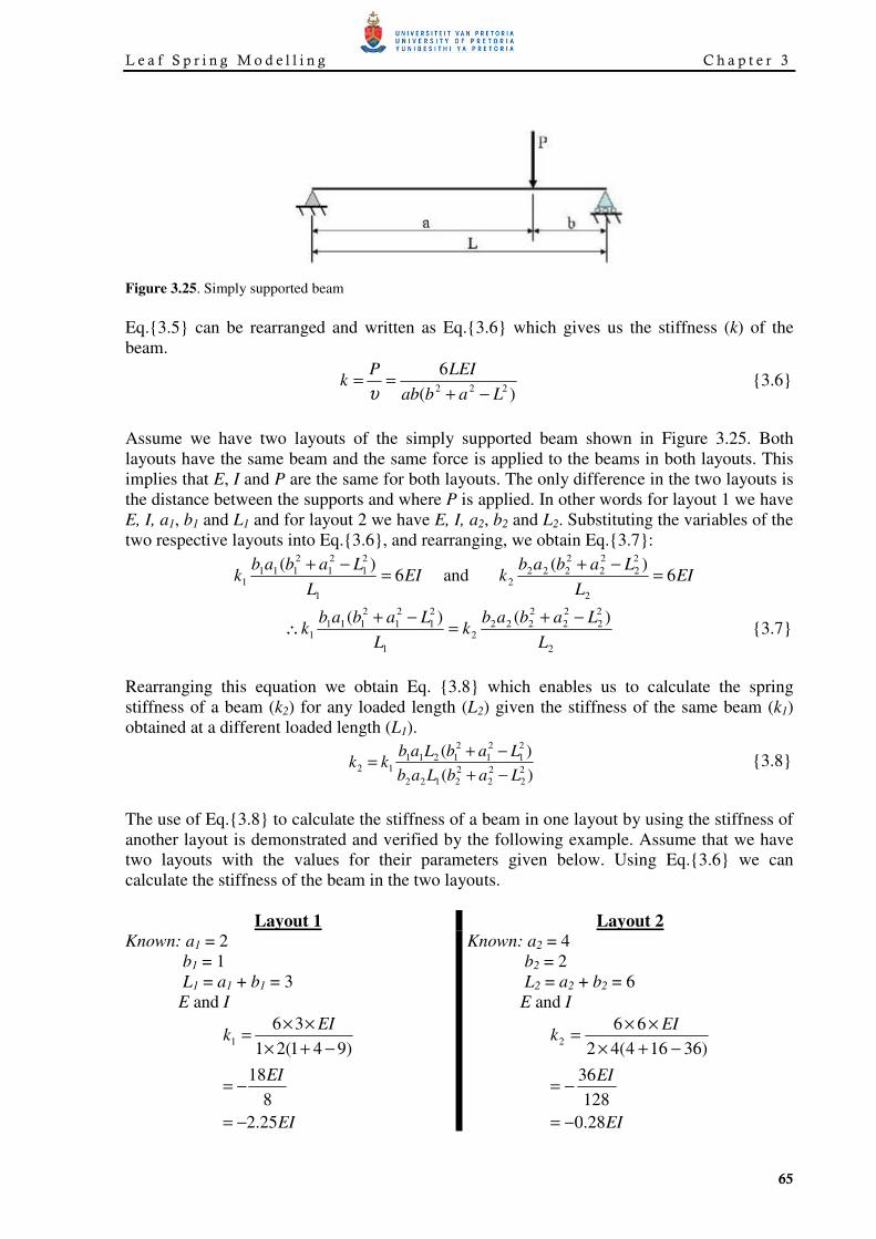
spring is based on beam theory. Consider the beam shown in Figure 3.25. Gere (2004) gives

Eq.{3.5} to calculate the deflection of the beam at the point where the force (P) is applied.

)(6

222xbL

LEI

Pbx−−−=υ )0( ax ≤≤ {3.5}


65

Figure 3.25. Simply supported beam

Eq.{3.5} can be rearranged and written as Eq.{3.6} which gives us the stiffness (k) of the

beam.

)(

6222

Labab

LEIPk

−+==

υ {3.6}

Assume we have two layouts of the simply supported beam shown in Figure 3.25. Both

layouts have the same beam and the same force is applied to the beams in both layouts. This

implies that E, I and P are the same for both layouts. The only difference in the two layouts is

the distance between the supports and where P is applied. In other words for layout 1 we have

E, I, a1, b1 and L1 and for layout 2 we have E, I, a2, b2 and L2. Substituting the variables of the

two respective layouts into Eq.{3.6}, and rearranging, we obtain Eq.{3.7}:

EIL

Lababk 6

)(

1

2

1

2

1

2

1111 =

−+ and EI

L

Lababk 6

)(

2

2

2

2

2

2

2222 =

−+

2

2

2

2

2

2

2222

1

2

1

2

1

2

1111

)()(

L

Lababk

L

Lababk

−+=

−+∴ {3.7}

Rearranging this equation we obtain Eq. {3.8} which enables us to calculate the spring

stiffness of a beam (k2) for any loaded length (L2) given the stiffness of the same beam (k1)

obtained at a different loaded length (L1).

)(

)(2

2

2

2

2

2122

2

1

2

1

2

121112

LabLab

LabLabkk

−+

−+= {3.8}

The use of Eq.{3.8} to calculate the stiffness of a beam in one layout by using the stiffness of

another layout is demonstrated and verified by the following example. Assume that we have

two layouts with the values for their parameters given below. Using Eq.{3.6} we can

calculate the stiffness of the beam in the two layouts.

Layout 1 Layout 2

Known: a1 = 2

b1 = 1

L1 = a1 + b1 = 3

E and I

EI

EI

EIk

25.2

8

18

)941(21

361

−=

−=

−+×

××=

Known: a2 = 4

b2 = 2

L2 = a2 + b2 = 6

E and I

EI

EI

EIk

28.0

128

36

)36164(42

662

−=

−=

−+×

××=


66

Now let’s approach this problem from a different angle. We would like to calculate the

stiffness of the beam in layout 2 but we do not know the young’s modules (E) or the inertia (I)

of the beam. However, we have the same beam in both layouts and we know the stiffness (k1),

and the length between the supports (L1, L2) and the application point (a1, b1, a2, b2) of the

force (P) for both layouts. In this situation we cannot use Eq.{3.6} to calculate the stiffness of

the beam as we do not know the young’s modules (E) of the material or the inertia (I) of the

beam. However, the information that is known makes it possible to use Eq.{3.8} to calculate

the stiffness of the beam in layout 2.

Known: k1 = -2.25EI

a1 = 2

b1 = 1

L1 = a1 + b1 = 3

a2 = 4

b2 = 2

L2 = a2 + b2 = 6

Substituting the known values into Eq.{3.8} we obtain:

EIk 28.02 −=

This is the same result as obtained when using Eq.{3.6}. Eq.{3.8} gives a simple method that

relates the stiffness of the leaf spring to its loaded length. This method makes it possible to

recalculate the experimentally extracted stiffnesses (k, kUL and kL), needed for the elasto-

plastic leaf spring model, obtained from one layout to other layouts. This implies that the

force-displacement characteristic only have to be obtained for one layout. To verify this the

elasto-plastic leaf spring model is combined with Eq.{3.8} to check whether this combined

model can indeed capture the change in stiffness for different loaded lengths. The predictions

from the combined model for both the multi-leaf spring and parabolic leaf spring are

compared to the experimental data obtained in Chapter 2. The validation results are presented

in the following paragraph.

4.2. Validation of loaded length calculation combined with EPLS

model

The combination of the proposed method for accounting for a change in loaded length and the

elastic-linear version of the EPLS model will now be validated against measured data. The

model will be used to predict the force-displacement characteristic of both the multi-leaf

spring and the parabolic leaf spring’s behaviour that was experimentally obtained in Chapter

2. The results from the model will be validated against these experimental measurements. The

loaded length was changed in the experimental setup by changing the longitudinal spacing of

the hangers. The experimental force-displacement characteristic, for both the multi-leaf spring

and parabolic leaf spring, were obtained at seven different spacings as was shown in Chapter

2. Four of these seven layouts will be used to validate the combined model. Table 3.4 shows

the dimensions of the four layouts that are used. The layout at the normal position is used to

extract the stiffnesses (k, kUL and kL) of the spring as needed to define the elastic-plastic

formulation of the EPLS model. These stiffnesses along with the loaded length of the other

layouts are then given to the combined model. The results for the multi-leaf spring and the

parabolic leaf spring are given in the following two paragraphs.


67

Table 3.4. Dimensions of layouts (see Figure 3.24)

Position Layout Front spacing (a)

[mm]

Rear spacing (b)

[mm]

Loaded length (L)

[mm]

Normal Original 510 478 988

Min 1 430 398 828

Pos3 2 490 458 908

Pos5 3 530 518 1048

4.2.1. Multi-leaf spring

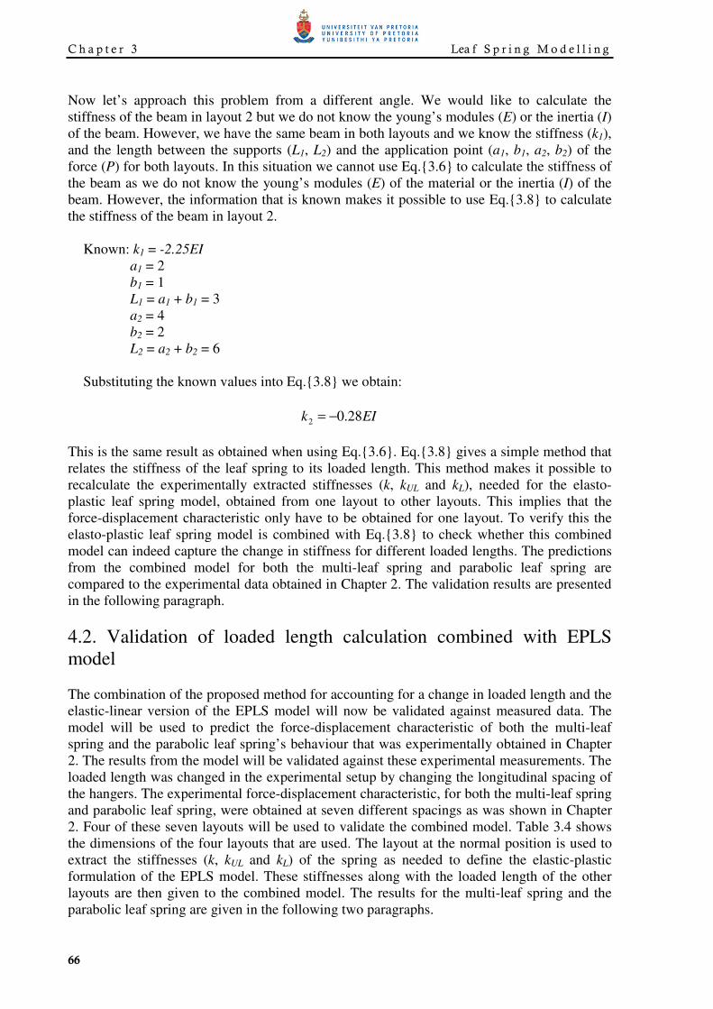
Figure 3.26 shows the comparison between the predicted and measured force-displacement

characteristic of the multi-leaf spring. From the figure the effect of the loaded length on the

stiffness of the multi-leaf spring can clearly be observed. The stiffness decreases from Lay 1

to Lay 3 as the loaded length increases. From the comparisons it is evident that Eq. {3.8}

combined with the linear-elastic formulation of the EPLS model gives accurate predictions of

the multi-leaf spring’s characteristics for different loaded lengths.

Figure 3.26. Comparison of measured and predicted force-displacement characteristics of multi-leaf spring for

different loaded lengths

4.2.2. Parabolic leaf spring

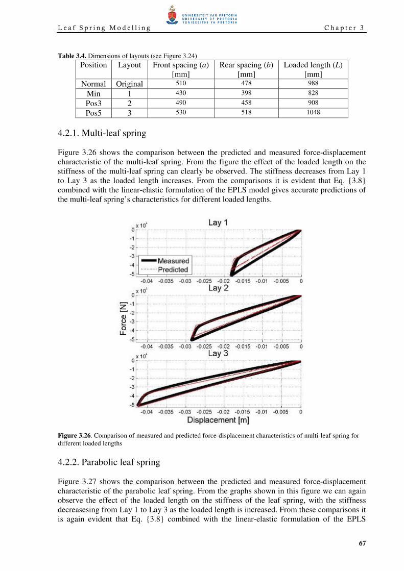
Figure 3.27 shows the comparison between the predicted and measured force-displacement

characteristic of the parabolic leaf spring. From the graphs shown in this figure we can again

observe the effect of the loaded length on the stiffness of the leaf spring, with the stiffness

decreasesing from Lay 1 to Lay 3 as the loaded length is increased. From these comparisons it

is again evident that Eq. {3.8} combined with the linear-elastic formulation of the EPLS


68

model gives accurate predictions of the parabolic leaf spring’s characteristics for different

loaded lengths.

Figure 3.27. Comparison of measured and predicted force-displacement characteristics of parabolic leaf spring

for different loaded lengths

4.3. Conclusion

The method that was proposed to account for changes in the loaded length was combined with

the linear-elastic leaf spring model. This combination was used to predict the characteristics

of different layouts of a multi-leaf spring as well as a parabolic leaf spring. The predicted

characteristics were compared to measured characteristics and showed good correlation. The

combined model was shown here to work for discrete changes in the loaded length. It should

be confirmed that this combined model is also capable of predicting the force-displacement

characteristic for a continuous change in the loaded length.

Up to this point we have shown that the physics-based EPLS model is able to emulate both

the multi-leaf spring as well as the parabolic leaf spring. The EPLS model was combined with

a method that is able to capture the sensitivity of the stiffness with respect to the loaded

length. Attention will now be given to the non-physics based neural network approach and its

ability to emulate the multi-leaf spring’s vertical behaviour.


69

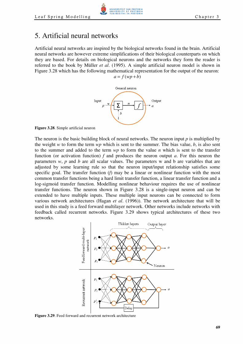
5. Artificial neural networks

Artificial neural networks are inspired by the biological networks found in the brain. Artificial

neural networks are however extreme simplifications of their biological counterparts on which

they are based. For details on biological neurons and the networks they form the reader is

referred to the book by Müller et al. (1995). A simple artificial neuron model is shown in

Figure 3.28 which has the following mathematical representation for the output of the neuron:

)( bwpfa +=

Figure 3.28. Simple artificial neuron

The neuron is the basic building block of neural networks. The neuron input p is multiplied by

the weight w to form the term wp which is sent to the summer. The bias value, b, is also sent

to the summer and added to the term wp to form the value n which is sent to the transfer

function (or activation function) f and produces the neuron output a. For this neuron the

parameters w, p and b are all scalar values. The parameters w and b are variables that are

adjusted by some learning rule so that the neuron input/input relationship satisfies some

specific goal. The transfer function (f) may be a linear or nonlinear function with the most

common transfer functions being a hard limit transfer function, a linear transfer function and a

log-sigmoid transfer function. Modelling nonlinear behaviour requires the use of nonlinear

transfer functions. The neuron shown in Figure 3.28 is a single-input neuron and can be

extended to have multiple inputs. These multiple input neurons can be connected to form

various network architectures (Hagan et al. (1996)). The network architecture that will be

used in this study is a feed forward multilayer network. Other networks include networks with

feedback called recurrent networks. Figure 3.29 shows typical architectures of these two

networks.

Figure 3.29. Feed forward and recurrent network architecture


70

5.1. Neural network model

This study will look at employing artificial neural networks in modelling the vertical

behaviour of the multi-leaf spring. The literature study in Chapter 1 showed that neural

networks have been used successfully to emulate the vertical behaviour of a leaf spring. Ghazi

Zadeh et al (2000) used two similar recurrent neural networks with one emulating the loading

behaviour and the other one the unloading behaviour of the leaf spring. A switching algorithm

was used to determine which one of the networks should be used depending on whether the

spring is loaded or unloaded. Each of the loading and unloading neural networks has

architecture of 3 x 10 x 20 x 1. The three inputs to the neural network are the deflection at the

current time step, the absolute value of the deflection change and the force at the previous

time step (this is the recurrent terminal). The required training data was generated by an

analytical model of the leaf spring.

Before going to a recurrent network architecture, such as used in the study by Ghazi Zadeh et

al.(2000), a simple feed forward network architecture will be used to emulate the force-

displacement characteristics of the multi-leaf spring. The advantage of using a feed forward

network over a recurrent network is that the training of the feed forward network is faster. The

feed forward neural network that is used in this study has two inputs being the displacement

and the velocity of the spring with the output being the spring force. The architecture of the

feed forward neural network is 2 x 35 x 1. The hidden layer has 35 neurons with a tan-

sigmoid (tansig) transfer function with the output layer having a linear (purelin) activation

function. The network is shown in Figure 3.30.

Figure 3.30. The 2-35-1 network

There is no clear method in which the architecture of a neural network can be determined.

There are however some general guidelines which can be followed to obtain a good neural

network. For instance, these guidelines give an indication of the amount of neurons that

should be used in order to obtain good generalization from the neural network. The choice of

the network architecture shown in Figure 3.30 was based on the following considerations. The

choice in using the displacement as input is obvious as any spring develops a force due to it

being deflected. The velocity is chosen as this will tell the neural network whether its being

loaded or unloaded. The nonlinear function that will be required to model the force-

displacement is not that complex and it is assumed that 35 neurons will be a good starting

point.

The 2-35-1 neural network is a much simpler network than was used in the study of Ghazi

Zadeh et al. (2000). Furthermore, instead of obtaining the training data from an analytical leaf

spring model, as was the case in the study of Ghazi Zadeh et al. (2000), the training data is

obtained from the experimental measurements on the leaf spring from Chapter 2. The multi-


71

leaf spring in the spring only setup will be used to evaluate whether the 2-35-1 neural network

can emulate the multi-leaf spring.

Two training sets were constructed from the experimental data. The first training set used data

that consisted of only the outer force-displacement loop. The second training set used data

that consisted of all the loops in the force-displacement characteristic that are the result of

different combinations of static loads and amplitudes. Figure 3.31 indicates the loops

mentioned above.

Figure 3.31. The different loops are shown on the force-displacement characteristic in (a) and, on the force and

displacements versus data points in (b)

Two 2-35-1 neural networks were trained, one using the first training data set and the other

using the second training data set. Both neural networks were then simulated by giving them

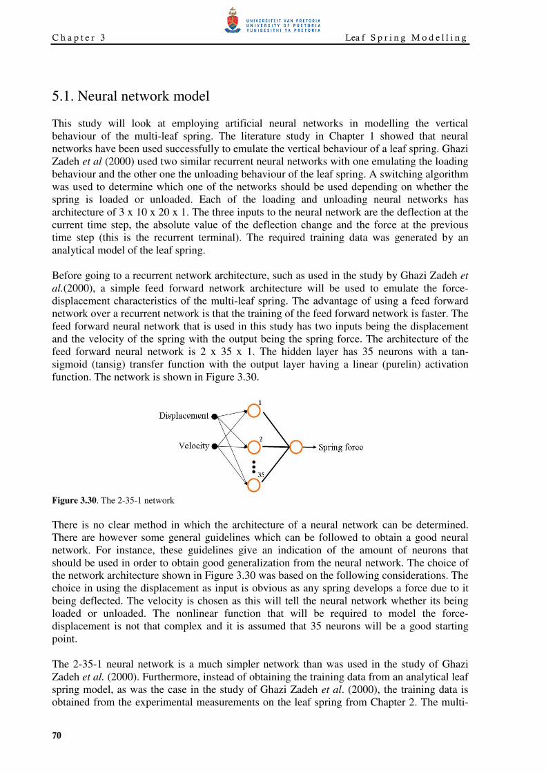
the same displacement input signal. Figure 3.32 shows the results of the neural network

compared to the experimental data when the first training set is used. From this figure it can

be observed that the neural network emulates the leaf spring well for the outer loop, however,

for the other loops it gives inaccurate predictions. The outer loop, for which good correlation

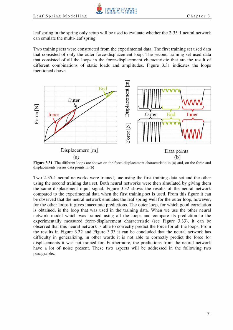
is obtained, is the loop that was used in the training data. When we use the other neural

network model which was trained using all the loops and compare its prediction to the

experimentally measured force-displacement characteristic (see Figure 3.33), it can be

observed that this neural network is able to correctly predict the force for all the loops. From

the results in Figure 3.32 and Figure 3.33 it can be concluded that the neural network has

difficulty in generalizing, in other words it is not able to correctly predict the force for

displacements it was not trained for. Furthermore, the predictions from the neural network

have a lot of noise present. These two aspects will be addressed in the following two

paragraphs.


72

Figure 3.32. Comparison of neural network predictions and experimental data (neural network trained with outer

loop)

Figure 3.33. Comparison of neural network predictions and experimental data (neural network trained with all

loops)

5.1.1. Reducing noise on neural network predictions

The results shown in Figure 3.33 showed that the neural network was able to predict the

spring force due to a given displacement when it was trained with data that covered the entire

working range of the function variables (in this case the displacement and velocity). The

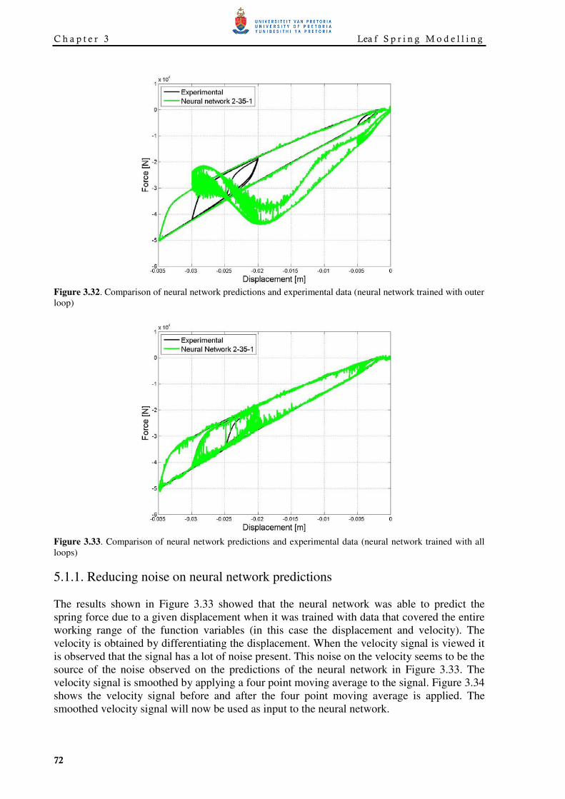
velocity is obtained by differentiating the displacement. When the velocity signal is viewed it

is observed that the signal has a lot of noise present. This noise on the velocity seems to be the

source of the noise observed on the predictions of the neural network in Figure 3.33. The

velocity signal is smoothed by applying a four point moving average to the signal. Figure 3.34

shows the velocity signal before and after the four point moving average is applied. The

smoothed velocity signal will now be used as input to the neural network.


73

Figure 3.34. Velocity signal before and after smoothing

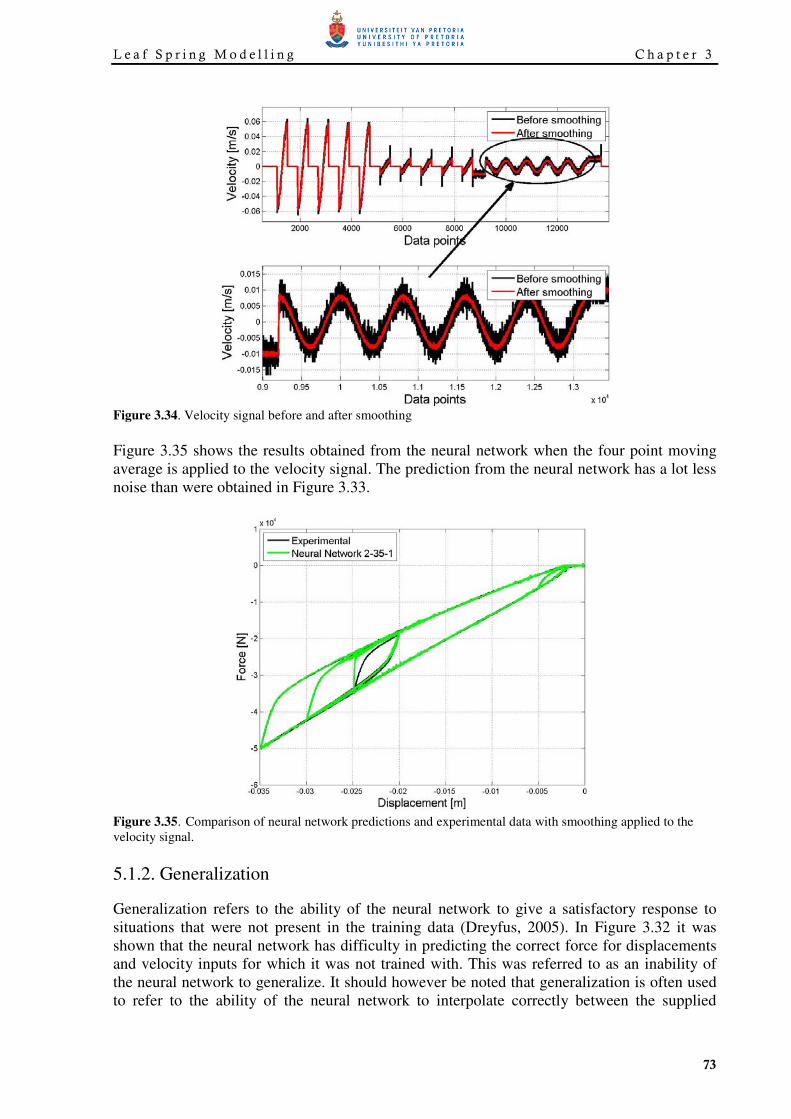
Figure 3.35 shows the results obtained from the neural network when the four point moving

average is applied to the velocity signal. The prediction from the neural network has a lot less

noise than were obtained in Figure 3.33.

Figure 3.35. Comparison of neural network predictions and experimental data with smoothing applied to the

velocity signal.

5.1.2. Generalization

Generalization refers to the ability of the neural network to give a satisfactory response to

situations that were not present in the training data (Dreyfus, 2005). In Figure 3.32 it was

shown that the neural network has difficulty in predicting the correct force for displacements

and velocity inputs for which it was not trained with. This was referred to as an inability of

the neural network to generalize. It should however be noted that generalization is often used

to refer to the ability of the neural network to interpolate correctly between the supplied


74

training data, whereas, in the case shown in Figure 3.32 the neural network is actually trying

to extrapolate.

The difference between the generalization ability of the neural network with respect to

interpolation and extrapolation is discussed using an example similar to the one used in Hagan

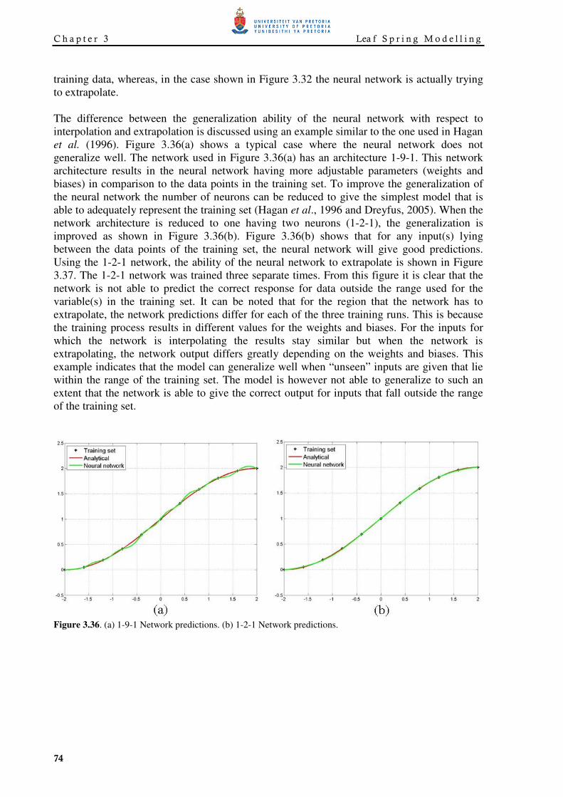
et al. (1996). Figure 3.36(a) shows a typical case where the neural network does not

generalize well. The network used in Figure 3.36(a) has an architecture 1-9-1. This network

architecture results in the neural network having more adjustable parameters (weights and

biases) in comparison to the data points in the training set. To improve the generalization of

the neural network the number of neurons can be reduced to give the simplest model that is

able to adequately represent the training set (Hagan et al., 1996 and Dreyfus, 2005). When the

network architecture is reduced to one having two neurons (1-2-1), the generalization is

improved as shown in Figure 3.36(b). Figure 3.36(b) shows that for any input(s) lying

between the data points of the training set, the neural network will give good predictions.

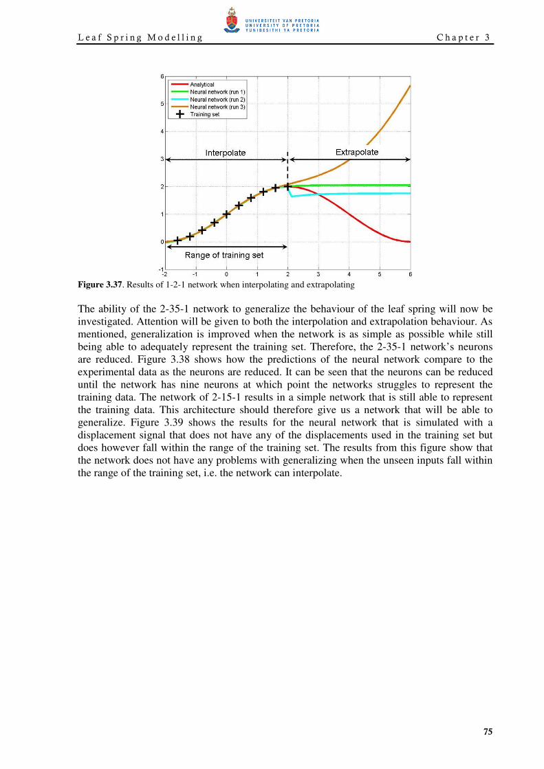
Using the 1-2-1 network, the ability of the neural network to extrapolate is shown in Figure

3.37. The 1-2-1 network was trained three separate times. From this figure it is clear that the

network is not able to predict the correct response for data outside the range used for the

variable(s) in the training set. It can be noted that for the region that the network has to

extrapolate, the network predictions differ for each of the three training runs. This is because

the training process results in different values for the weights and biases. For the inputs for

which the network is interpolating the results stay similar but when the network is

extrapolating, the network output differs greatly depending on the weights and biases. This

example indicates that the model can generalize well when “unseen” inputs are given that lie

within the range of the training set. The model is however not able to generalize to such an

extent that the network is able to give the correct output for inputs that fall outside the range

of the training set.

Figure 3.36. (a) 1-9-1 Network predictions. (b) 1-2-1 Network predictions.


75

Figure 3.37. Results of 1-2-1 network when interpolating and extrapolating

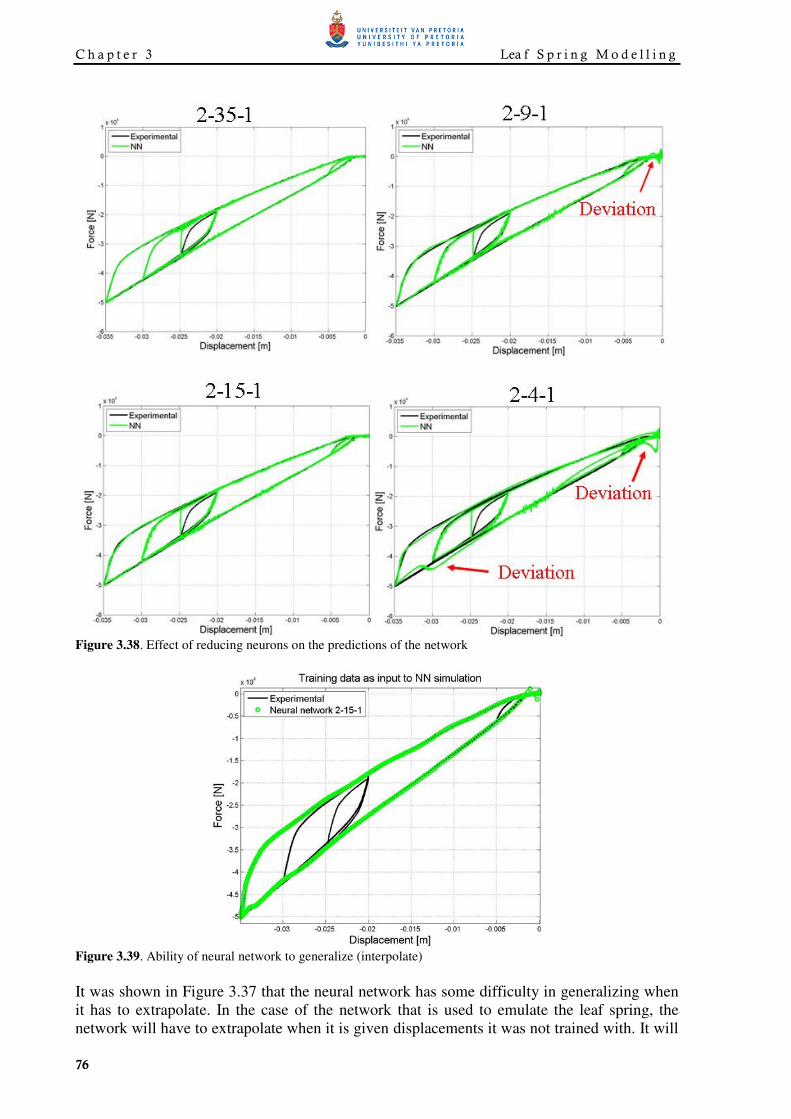
The ability of the 2-35-1 network to generalize the behaviour of the leaf spring will now be

investigated. Attention will be given to both the interpolation and extrapolation behaviour. As

mentioned, generalization is improved when the network is as simple as possible while still

being able to adequately represent the training set. Therefore, the 2-35-1 network’s neurons

are reduced. Figure 3.38 shows how the predictions of the neural network compare to the

experimental data as the neurons are reduced. It can be seen that the neurons can be reduced

until the network has nine neurons at which point the networks struggles to represent the

training data. The network of 2-15-1 results in a simple network that is still able to represent

the training data. This architecture should therefore give us a network that will be able to

generalize. Figure 3.39 shows the results for the neural network that is simulated with a

displacement signal that does not have any of the displacements used in the training set but

does however fall within the range of the training set. The results from this figure show that

the network does not have any problems with generalizing when the unseen inputs fall within

the range of the training set, i.e. the network can interpolate.


76

Figure 3.38. Effect of reducing neurons on the predictions of the network

Figure 3.39. Ability of neural network to generalize (interpolate)

It was shown in Figure 3.37 that the neural network has some difficulty in generalizing when

it has to extrapolate. In the case of the network that is used to emulate the leaf spring, the

network will have to extrapolate when it is given displacements it was not trained with. It will


77

also have to extrapolate when the network is given displacements that it has been trained with

but have a different excitation frequency. This dependency on frequency is present due to the

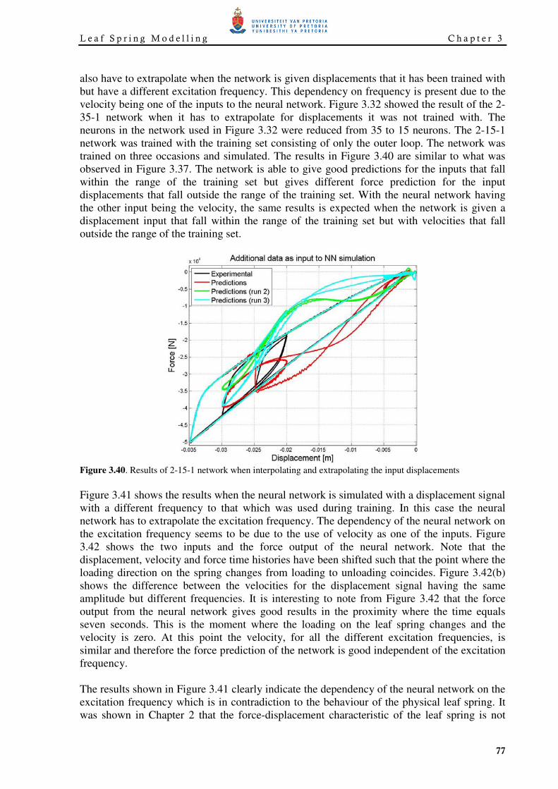
velocity being one of the inputs to the neural network. Figure 3.32 showed the result of the 2-

35-1 network when it has to extrapolate for displacements it was not trained with. The

neurons in the network used in Figure 3.32 were reduced from 35 to 15 neurons. The 2-15-1

network was trained with the training set consisting of only the outer loop. The network was

trained on three occasions and simulated. The results in Figure 3.40 are similar to what was

observed in Figure 3.37. The network is able to give good predictions for the inputs that fall

within the range of the training set but gives different force prediction for the input

displacements that fall outside the range of the training set. With the neural network having

the other input being the velocity, the same results is expected when the network is given a

displacement input that fall within the range of the training set but with velocities that fall

outside the range of the training set.

Figure 3.40. Results of 2-15-1 network when interpolating and extrapolating the input displacements

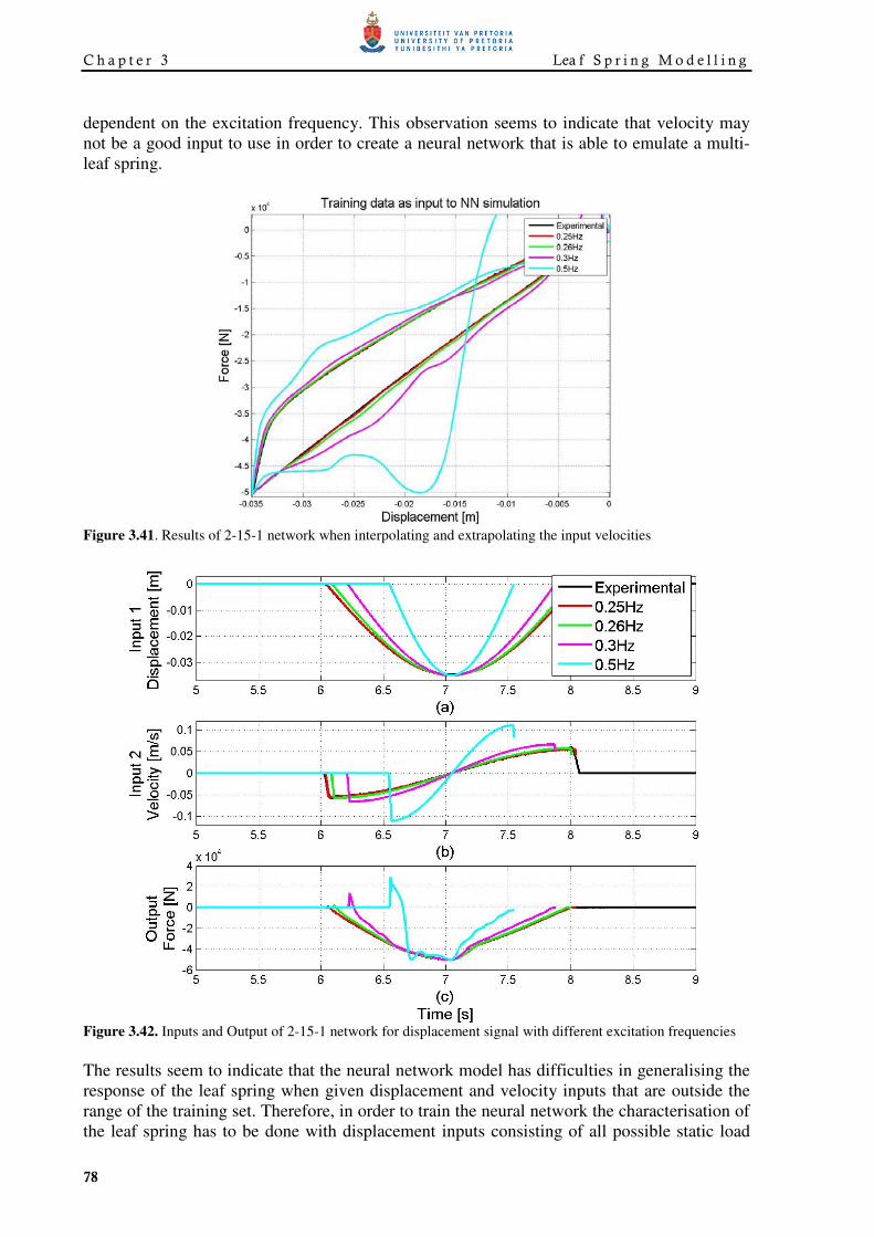
Figure 3.41 shows the results when the neural network is simulated with a displacement signal

with a different frequency to that which was used during training. In this case the neural

network has to extrapolate the excitation frequency. The dependency of the neural network on

the excitation frequency seems to be due to the use of velocity as one of the inputs. Figure

3.42 shows the two inputs and the force output of the neural network. Note that the

displacement, velocity and force time histories have been shifted such that the point where the

loading direction on the spring changes from loading to unloading coincides. Figure 3.42(b)

shows the difference between the velocities for the displacement signal having the same

amplitude but different frequencies. It is interesting to note from Figure 3.42 that the force

output from the neural network gives good results in the proximity where the time equals

seven seconds. This is the moment where the loading on the leaf spring changes and the

velocity is zero. At this point the velocity, for all the different excitation frequencies, is

similar and therefore the force prediction of the network is good independent of the excitation

frequency.

The results shown in Figure 3.41 clearly indicate the dependency of the neural network on the

excitation frequency which is in contradiction to the behaviour of the physical leaf spring. It

was shown in Chapter 2 that the force-displacement characteristic of the leaf spring is not


78

dependent on the excitation frequency. This observation seems to indicate that velocity may

not be a good input to use in order to create a neural network that is able to emulate a multi-

leaf spring.

Figure 3.41. Results of 2-15-1 network when interpolating and extrapolating the input velocities

Figure 3.42. Inputs and Output of 2-15-1 network for displacement signal with different excitation frequencies

The results seem to indicate that the neural network model has difficulties in generalising the

response of the leaf spring when given displacement and velocity inputs that are outside the

range of the training set. Therefore, in order to train the neural network the characterisation of

the leaf spring has to be done with displacement inputs consisting of all possible static load


79

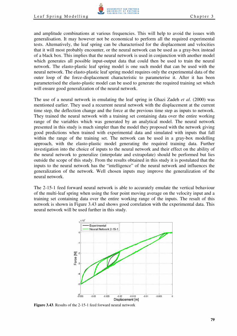
and amplitude combinations at various frequencies. This will help to avoid the issues with

generalisation. It may however not be economical to perform all the required experimental

tests. Alternatively, the leaf spring can be characterised for the displacement and velocities

that it will most probably encounter, or the neural network can be used as a gray-box instead

of a black box. This implies that the neural network is used in conjunction with another model

which generates all possible input-output data that could then be used to train the neural

network. The elasto-plastic leaf spring model is one such model that can be used with the

neural network. The elasto-plastic leaf spring model requires only the experimental data of the

outer loop of the force-displacement characteristic to parameterise it. After it has been

parameterised the elasto-plastic model can be used to generate the required training set which

will ensure good generalization of the neural network.

The use of a neural network in emulating the leaf spring in Ghazi Zadeh et al. (2000) was

mentioned earlier. They used a recurrent neural network with the displacement at the current

time step, the deflection change and the force at the previous time step as inputs to network.

They trained the neural network with a training set containing data over the entire working

range of the variables which was generated by an analytical model. The neural network

presented in this study is much simpler than the model they proposed with the network giving

good predictions when trained with experimental data and simulated with inputs that fall

within the range of the training set. The network can be used in a gray-box modelling

approach, with the elasto-plastic model generating the required training data. Further

investigation into the choice of inputs to the neural network and their effect on the ability of

the neural network to generalize (interpolate and extrapolate) should be performed but lies

outside the scope of this study. From the results obtained in this study it is postulated that the

inputs to the neural network has the “intelligence” of the neural network and influences the

generalization of the network. Well chosen inputs may improve the generalization of the

neural network.

The 2-15-1 feed forward neural network is able to accurately emulate the vertical behaviour

of the multi-leaf spring when using the four point moving average on the velocity input and a

training set containing data over the entire working range of the inputs. The result of this

network is shown in Figure 3.43 and shows good correlation with the experimental data. This

neural network will be used further in this study.

Figure 3.43. Results of the 2-15-1 feed forward neural network


80

6. Conclusion

This chapter was concerned with the modelling of the vertical behaviour of the leaf spring. A

novel physics-based model was developed that is able to capture the complex nonlinear

hysteric behaviour of the leaf spring. The capability of the elasto-plastic leaf spring model to

represent both the multi-leaf spring and the parabolic leaf spring was shown. A simple

modelling technique was also presented in order to capture the changes in stiffness of the leaf

spring due to changes in the loaded length of the leaf spring. The non-physics based neural

network approach was also investigated. It was found that the neural network was able to

emulate the vertical behaviour of the leaf spring when trained with data over the entire range

of the variables.

The next chapter will see the use of the elasto-plastic leaf spring model in creating a model of

the simplified version of the suspension system used during the characterisation in Chapter 2.

This is according to the systematic approach which sees an incremental increase in

complexity of models with validation at each stage. A comparison between the accuracy and

efficiency of the elasto-plastic and the neural network model of the multi-leaf spring will be

shown in Chapter 5 after the modified percentage relative error validation metric has been

introduced.

Documents

Leaf spring modelling