Embed Size (px)
Citation preview

Leaky aquiferLeaky aquifer
Aquifers which are overlain or underlain by semi permeable
strata are referred to as leaky Aquifers. In such aquifers
significant portion of the yield may be derived by vertical
leakage
• aquifer has infinite areal extent
• aquifer is homogeneous, isotropic and of uniform thickness
• pumping well is fully penetrating
• flow to pumping well is horizontal when pumping well is fully penetrating
• aquifer is leaky
• flow is unsteady
AssumptionsAssumptions•water is released instantaneously from storage with decline of hydraulic head
•diameter of pumping well is very small so that storage in the well can be neglected
•confining bed(s) has infinite areal extent, uniform vertical hydraulic conductivity and uniform thickness
•confining bed(s) is overlain or underlain by an infinite constant-head plane source
•flow in the aquitard(s) is vertical
a. Unconfined aquifer is recharged by lower confined aquifer
The velocity (v) of the downward or upward vertical flow(
Leakage) through the semi confining layer is proportional to to the
difference between groundwater table and piezometric head in the
Confined layers, which can be calculated by Darcy law.
B. Unconfined aquifer is recharging Lower confined aquifer
d. Upper confined aquifer is
Recharging lower confined aquiferc. Lower confined aquifer is recharging upper confined aquifer

E confined aquifer is rechargedFrom top unconfined and bottomConfined aquifer
Confined aquifer is recharge bothFrom top and bottom confined aquifers
Total vertical leakage Qe)
Qe= v*Ae or
Qe= (K’/b’)* Delta h*Ae
K’/b’ is called leakance and its reciprocal b’/K’
Is called hydraulic resistance “c” of the confining
Layer
Sq.root 0f (T*c) is called leakage factor B
The velocity (v) of the downward/ upward vertical flow(
Leakage) through the semi confining layer is proportional
to to the difference between groundwater table and
piezometric head in the Confined layers, which can be
calculated by Darcy law.
v= K’ Delta h/b’
Leakage is more near pumping well than far away as
Delta h is more Near pumping well
(((( ))))'b'KTB ====
Flow in leaky confined aquiferFlow in leaky confined aquifer
Unsteady state radial flow
Flow in leaky confined aquiferFlow in leaky confined aquifer
Unsteady state Radial flow

(((( ))))Br,uW
T4
Qs
ππππ====
(((( ))))'b'KTB ====
Type curves for leaky aquifersType curves for leaky aquifers
Example1Example1
The time drawdown data for unsteady flow in an observation well at 30 m from
Pumping well is given below. Q= 800 lpm. The thick ness of the aquifer is 12 m.
The thick ness of leaky aquifer is 4.0 m. Determine the aquifer parameters.
Time since
pumping
started (mts)
Drawdown
(m)
5 0.25
10 0.5
30 1.00
60 1.32
100 1.6
200 1.7
400 1.8
600 1.83
800 1.88
1000 1.91
1200 1.92
Data plot matched with r/B=0.2
The match point data is
W(u.r/B)= 3.5
1/u= 380
s= 1.91m
t= 1000mts
R= 30m
Q= 800lpm
b= 12 m
b’= 4m
(((( ))))Br,uW
T4
Qs
ππππ====
(((( ))))'b'KTB ====
where
T= 168 SQ.M/DAY
S=0.0014r/B=0.2B= 150 mC= 135.5 daysK= 14.04 m/dayK’= 0.03 m/day

Flow in leaky confined aquiferFlow in leaky confined aquifer
Steady state Radial flow
s=( Q/2PIT)*K0(r/B)Where r/B= r/sqrt(T*C)
K0( r/B) = modified Bessel function of the second Kind and zero order.
Differential Equation- Bassel function
Solution
Bessel Function of the Second Kind (Neumann Functions)
Zero Order
where C = 0.577 215 665
Bessel Function of the First Kind
ZeroOrder
Bessel function
where n is a non-negative real number. The solutions of this equation are
called Bessel Functions of order n . Although the order can be any real
number, the scope of this section is limited to non-negative integers,
i.e., , unless specified otherwise.
Since Bessel's differential equation is a second order ordinary differential
equation, two sets of functions, the Bessel function of the first
kind and the Bessel function of the second kind (also known as the
Weber Function) , are needed to form the general solution:
First Kind Second kind

•Plot K0(r/B) vrs r/B on log log plot •Plot s versus r on log log plot and find match point •And calculate s, r, r/B and K0( r/B) and use the equation
s=( Q/2PIT)*K0(r/B)Where r/B= r/sqrt(T*C)
K0( r/B) = modified Bessel function of the second Kind and zero order.
Problemb= 30 mb’=10 mQ=1800 lpm
DradownsDis D/D(m)10 0.6620 0.5560 0.35100 0.26300 0.07
Calculate T KK’B
Steady state Radial flow- Leaky
Modified leaky equationModified leaky equation
If r/B <0.05, then the original equation can be modified To s= (2.3Q/2PI T)*log 1.12 B/r
T can be estimated from Distance Draw down curveB= r0*1.12C= r^2/(1.25*T)
Problemb= 30 mb’=10 mQ=1800 lpm
DradownsDis D/D(m)10 0.6620 0.5560 0.35100 0.26300 0.07
Calculate T KK’B
Steady state Radial flow- (Leaky) Distance - Drawdown
Hantush Inflection point methodHantush Inflection point methodHantush developed a method for estimating T and S and C by Plotting time drawdown on semi log paper and getting si, ti, andDelta si, i refers to the inflection point. That is the point where drawdown (si) is one half of the final drawdown given By the equation
s=( Q/2PIT)*K0(r/B)Where r/B= r/sqrt(T*C)
K0( r/B) = modified Bessel function of the second Kind and zero order.
And ui= r/2B r/2B= r^2*S/4Tti
2.3 * si/delta si= e^(r/B)*k0((r/B)
The slope of the curve at the inflection point Delta si is the drawdown per log cycle time and is give by
Delta si= 2.3 Q/4PiT*e^-r/BTherefore
Un Steady state Radial flow-Leaky
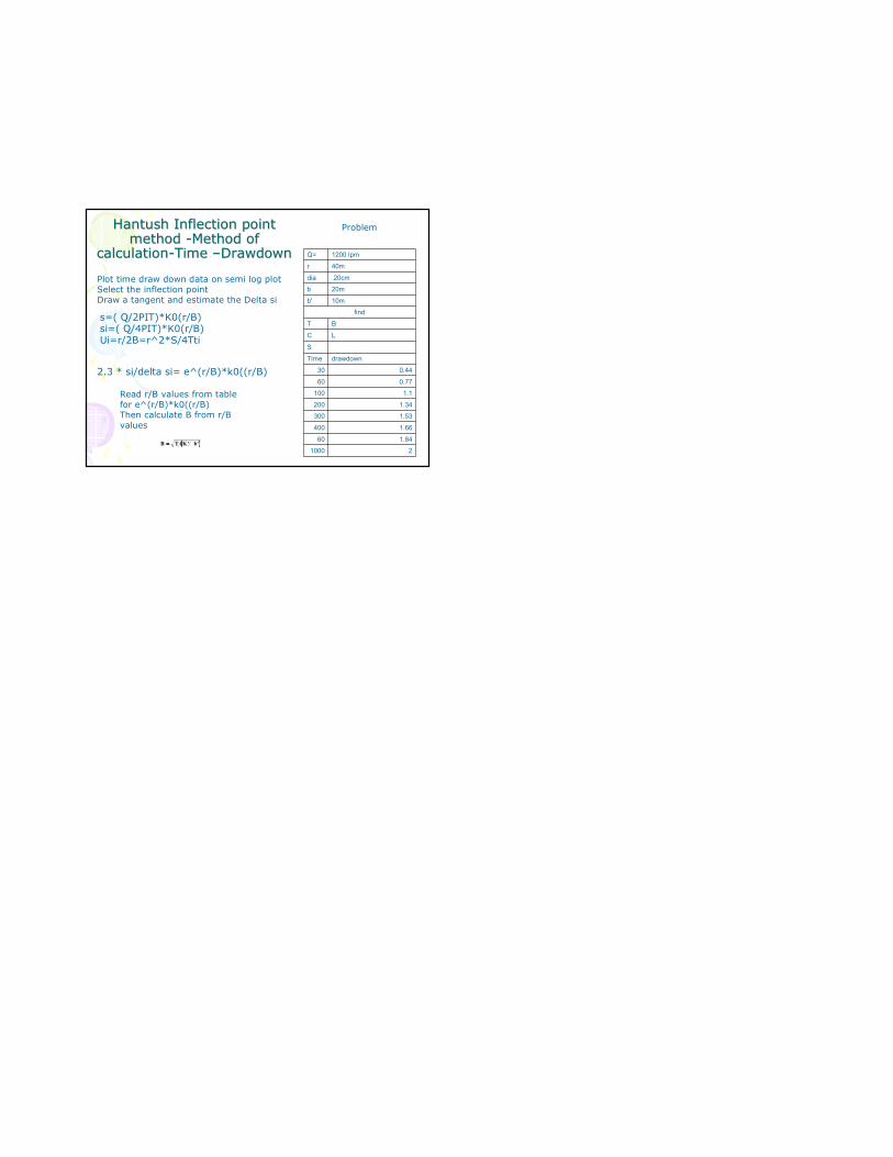
Hantush Inflection point Hantush Inflection point method method --Method of Method of
calculationcalculation--Time Time ––DrawdownDrawdown
(((( ))))'b'KTB ====
Plot time draw down data on semi log plotSelect the inflection pointDraw a tangent and estimate the Delta si
s=( Q/2PIT)*K0(r/B)si=( Q/4PIT)*K0(r/B)Ui=r/2B=r^2*S/4Tti
2.3 * si/delta si= e^(r/B)*k0((r/B)
Read r/B values from table for e^(r/B)*k0((r/B)Then calculate B from r/B values
Problem
Q= 1200 lpm
r 40m
dia .20cm
b 20m
b' 10m
find
T B
C L
S
Time drawdown
30 0.44
60 0.77
100 1.1
200 1.34
300 1.53
400 1.66
60 1.84
1000 2