Embed Size (px)
DESCRIPTION
LearnExcel
Citation preview

http://www.mrexcel.com/learn-excel.html
Learn Excel from Mr Excel - Week 10
Learn Excel from Mr ExcelCopyright 2005 Bill JelenAll Rights Reserved
Encourage your friends to sign up at
This week: There are three basic ways to enterformulas, and the method that you use says a lotabout how long you've been using spreadsheets.Read about all three methods in the first tip today,then vote about your favorite method athttp://www.mrexcel.com/formulapoll.php
The remaining three tips discuss AutoSum, why itdoesn't always work, other features in AutoSum, and why =COUNT() might be retuming the wrong results.
Part 2: calculating with excel
learn excel From mr excel
Part 2: calculating with excel
learn excel From mr excel
three MethodS oF entering ForMulAS
Problem: There are three basic ways of entering simple calculations in Excel. Knowing all three ways will allow you to enter formulas faster, according to the situation. Consider the worksheet shown in Fig. 336.
In Fig. 336, you want to calculate total cost in E3 as the Case Quantity in B3 times the Unit Cost in C3.Strategy: You can simply type the formula. 1) Put the cell pointer in E3 and type =b3*c3, as shown in Fig. 337,
and then hit Enter.
Fig. 336
Fig. 337
194

Part 2: calculating with excel
learn excel From mr excel
PartII
Part 2: calculating with excel
learn excel From mr excel
2) The formula will calculate. You will see the original formula in the formula bar above E1. The worksheet itself will show the result of the calculation, as shown in Fig. 338.
Advantage: If you are a good typist, you only need to type seven keystrokes. Disadvantage: This method gets complicated when you are dealing with complex formulas.Alternate Strategy: Use the arrow keys. Anyone who was using spread-sheets in the days of Lotus 1-2-3 often used this method. Once you have mastered this method, it is very fast and very intuitive.1) Move the cell pointer to E3. As shown in Fig. 339, type an Equal
sign to let Excel know that you are about to enter a formula.
Fig. 338
Fig. 339
195
Part 2: calculating with excel
learn excel From mr excel
Part 2: calculating with excel
learn excel From mr excel
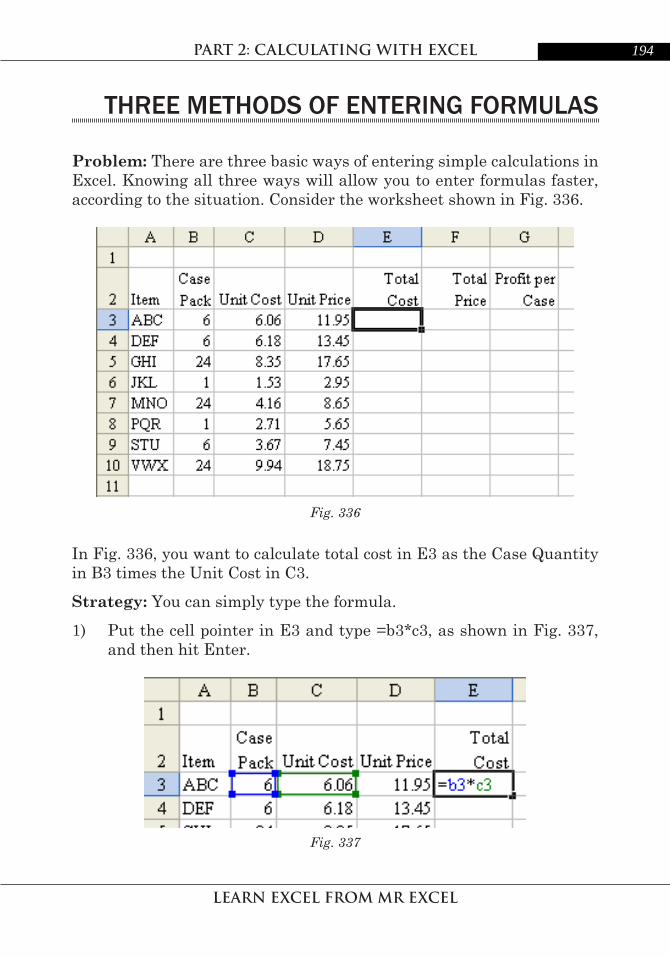
2) Hit the Left Arrow. As shown in Fig. 340, a dotted border surrounds the cell to the left of E3. Excel starts to build a formula of =D3.
3) Hit the Left Arrow key two more times. Your provisional formula is now =B3, as shown in Fig. 341.
4) On the keyboard, hit the * key. You can either hit Shift+8 or use the Asterisk key on the numeric keypad. The dotted border will disap-pear from B3 and be replaced by a solid-colored border, as shown in Fig. 342. Hitting any operator key, such as Plus, Minus, Asterisk, or Slash, tells Excel that you are moving on to the next part of the formula.
Fig. 340
Fig. 341
Fig. 342
196
Part 2: calculating with excel
learn excel From mr excel
PartII
Part 2: calculating with excel
learn excel From mr excel
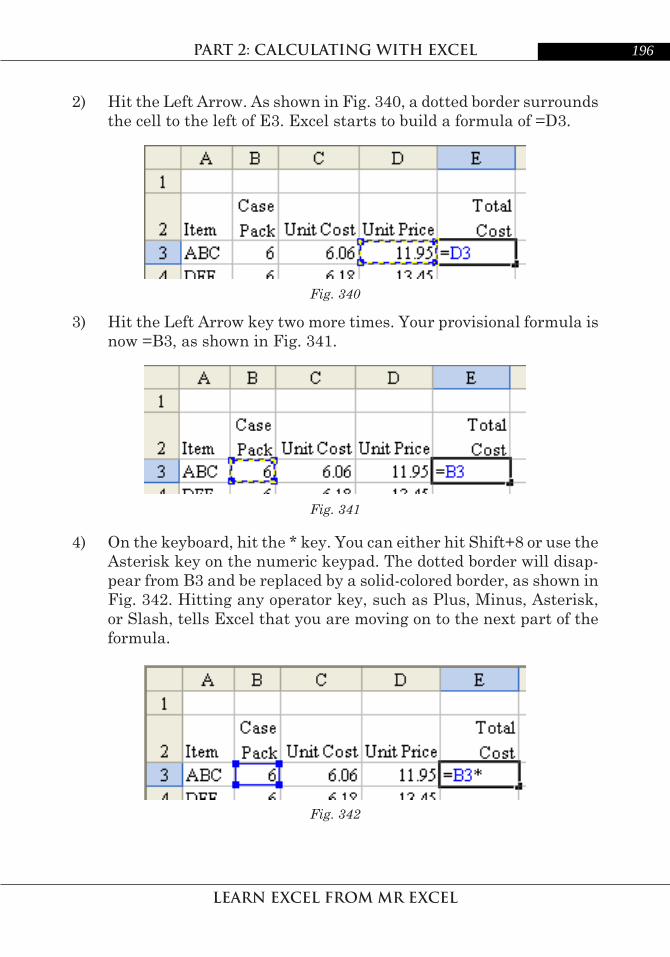
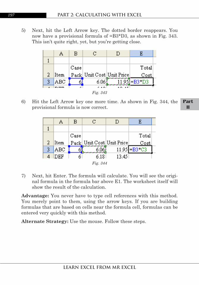
5) Next, hit the Left Arrow key. The dotted border reappears. You now have a provisional formula of =B3*D3, as shown in Fig. 343. This isn’t quite right, yet, but you’re getting close.
6) Hit the Left Arrow key one more time. As shown in Fig. 344, the provisional formula is now correct.
7) Next, hit Enter. The formula will calculate. You will see the origi-nal formula in the formula bar above E1. The worksheet itself will show the result of the calculation.
Advantage: You never have to type cell references with this method. You merely point to them, using the arrow keys. If you are building formulas that are based on cells near the formula cell, formulas can be entered very quickly with this method.Alternate Strategy: Use the mouse. Follow these steps.
Fig. 343
Fig. 344
197
Part 2: calculating with excel
learn excel From mr excel
Part 2: calculating with excel
learn excel From mr excel
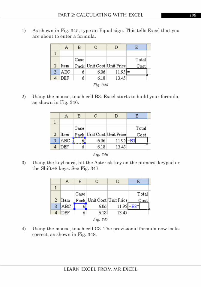
1) As shown in Fig. 345, type an Equal sign. This tells Excel that you are about to enter a formula.
2) Using the mouse, touch cell B3. Excel starts to build your formula, as shown in Fig. 346.
3) Using the keyboard, hit the Asterisk key on the numeric keypad or the Shift+8 keys. See Fig. 347.
4) Using the mouse, touch cell C3. The provisional formula now looks correct, as shown in Fig. 348.
Fig. 345
Fig. 346
Fig. 347
198

Part 2: calculating with excel
learn excel From mr excel
PartII
Part 2: calculating with excel
learn excel From mr excel
5) Hit the Enter key. The formula will calculate. You will see the orig-inal formula in the formula bar above E1. The worksheet itself will show the result of the calculation.
Advantages of the Mouse: It is easy to use the mouse to directly touch the cells you need in the formula.Disadvantage of the Mouse: It takes a long time to move your hands back and forth from the keyboard to the mouse. To enter the above for-mula, you have to hit a key, use the mouse, hit a key, use the mouse, and hit a key again. That is four movements back and forth from the keyboard to the mouse and back.Summary: There are three basic methods for entering formulas in Ex-cel. Using the right method for the situation can radically improve your efficiency.
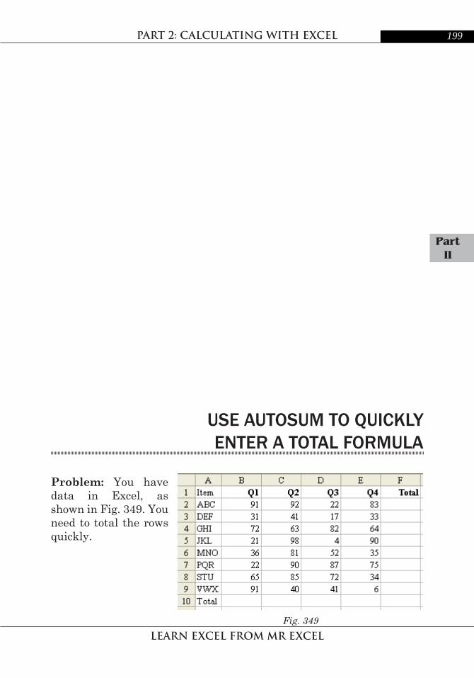
uSe AutoSuM to quiCkly enter A totAl ForMulA
Problem: You have data in Excel, as shown in Fig. 349. You need to total the rows quickly.
Fig. 348
Fig. 349
199
Part 2: calculating with excel
learn excel From mr excel
PartII
Part 2: calculating with excel
learn excel From mr excel
5) Hit the Enter key. The formula will calculate. You will see the orig-inal formula in the formula bar above E1. The worksheet itself will show the result of the calculation.
Advantages of the Mouse: It is easy to use the mouse to directly touch the cells you need in the formula.Disadvantage of the Mouse: It takes a long time to move your hands back and forth from the keyboard to the mouse. To enter the above for-mula, you have to hit a key, use the mouse, hit a key, use the mouse, and hit a key again. That is four movements back and forth from the keyboard to the mouse and back.Summary: There are three basic methods for entering formulas in Ex-cel. Using the right method for the situation can radically improve your efficiency.
uSe AutoSuM to quiCkly enter A totAl ForMulA
Problem: You have data in Excel, as shown in Fig. 349. You need to total the rows quickly.
Fig. 348
Fig. 349
199

Part 2: calculating with excel
learn excel From mr excel
Part 2: calculating with excel
learn excel From mr excel
Strategy: Use the AutoSum button on the Standard toolbar. The Auto-Sum button looks like the Greek letter sigma, as shown in Fig. 350.
1) Place the cell pointer in cell B10. Touch the AutoSum button, as shown in Fig. 351.
2) Excel analyzes your data and predicts that you want to total the range of num-bers above the cell point-er. As shown in Fig. 352, Excel enters a provisional formula of =SUM(B2:B9). Hit Enter to accept this formula.
Fig. 350
Fig. 351
Fig. 352
200
Part 2: calculating with excel
learn excel From mr excel
PartII
Part 2: calculating with excel
learn excel From mr excel
3) The square dot in the lower right corner of the cell pointer is the AutoFill handle. With the mouse, drag the Fill handle to the right to include cells C10 through F10. Release the mouse button and the formula will be copied to all five columns.
Summary: The AutoSum button on the Standard toolbar is a powerful tool for quickly entering a total formula.Functions Discussed: =SUM()
AutoSuM doeSn’t AlwAyS prediCt My dAtA CorreCtly
Problem: When using the AutoSum button, Excel sometimes predicts the wrong range of data to total. In Fig. 353, the AutoSum worked fine in F2 and F3, but in cell F4, Excel gets fooled into thinking that you want to total the rows above F4.
Strategy: After hitting the AutoSum button, the provisional range ad-dress is highlighted in the provisional formula. Using your mouse, high-light the right range.
Fig. 353
201

Part 2: calculating with excel
learn excel From mr excel
PartII
Part 2: calculating with excel
learn excel From mr excel
3) The square dot in the lower right corner of the cell pointer is the AutoFill handle. With the mouse, drag the Fill handle to the right to include cells C10 through F10. Release the mouse button and the formula will be copied to all five columns.
Summary: The AutoSum button on the Standard toolbar is a powerful tool for quickly entering a total formula.Functions Discussed: =SUM()
AutoSuM doeSn’t AlwAyS prediCt My dAtA CorreCtly
Problem: When using the AutoSum button, Excel sometimes predicts the wrong range of data to total. In Fig. 353, the AutoSum worked fine in F2 and F3, but in cell F4, Excel gets fooled into thinking that you want to total the rows above F4.
Strategy: After hitting the AutoSum button, the provisional range ad-dress is highlighted in the provisional formula. Using your mouse, high-light the right range.
Fig. 353
201
Part 2: calculating with excel
learn excel From mr excel
Part 2: calculating with excel
learn excel From mr excel
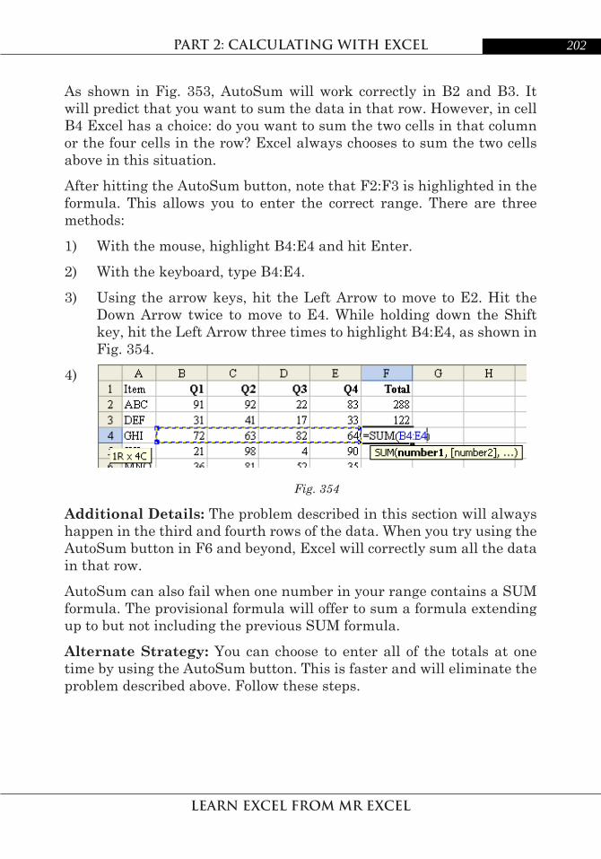
As shown in Fig. 353, AutoSum will work correctly in B2 and B3. It will predict that you want to sum the data in that row. However, in cell B4 Excel has a choice: do you want to sum the two cells in that column or the four cells in the row? Excel always chooses to sum the two cells above in this situation.After hitting the AutoSum button, note that F2:F3 is highlighted in the formula. This allows you to enter the correct range. There are three methods:1) With the mouse, highlight B4:E4 and hit Enter.2) With the keyboard, type B4:E4.3) Using the arrow keys, hit the Left Arrow to move to E2. Hit the
Down Arrow twice to move to E4. While holding down the Shift key, hit the Left Arrow three times to highlight B4:E4, as shown in Fig. 354.
4)
Fig. 354
Additional Details: The problem described in this section will always happen in the third and fourth rows of the data. When you try using the AutoSum button in F6 and beyond, Excel will correctly sum all the data in that row.AutoSum can also fail when one number in your range contains a SUM formula. The provisional formula will offer to sum a formula extending up to but not including the previous SUM formula.Alternate Strategy: You can choose to enter all of the totals at one time by using the AutoSum button. This is faster and will eliminate the problem described above. Follow these steps.
202

Part 2: calculating with excel
learn excel From mr excel
PartII
Part 2: calculating with excel
learn excel From mr excel
1) Highlight the entire range that needs a SUM formula as shown in Fig. 355.
2) Hit the AutoSum button. Excel makes a prediction and fills in the total formulas automatically, as shown in Fig. 356. Excel does not show the provisional formula. So, check one formula to see that it is correct.
Fig. 355
Fig. 356
203

Part 2: calculating with excel
learn excel From mr excel
Part 2: calculating with excel
learn excel From mr excel
Summary: The AutoSum function does not always correctly predict the range to be totaled. It is easy to use the mouse or keyboard to show Excel the correct range.Functions Discussed: =SUM()
uSe AutoSuM button to enter AVerAgeS, Min, MAx, And Count
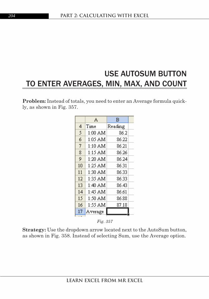
Problem: Instead of totals, you need to enter an Average formula quick-ly, as shown in Fig. 357.
Strategy: Use the dropdown arrow located next to the AutoSum button, as shown in Fig. 358. Instead of selecting Sum, use the Average option.
Fig. 357
204
Part 2: calculating with excel
learn excel From mr excel
Part 2: calculating with excel
learn excel From mr excel
Summary: The AutoSum function does not always correctly predict the range to be totaled. It is easy to use the mouse or keyboard to show Excel the correct range.Functions Discussed: =SUM()
uSe AutoSuM button to enter AVerAgeS, Min, MAx, And Count
Problem: Instead of totals, you need to enter an Average formula quick-ly, as shown in Fig. 357.
Strategy: Use the dropdown arrow located next to the AutoSum button, as shown in Fig. 358. Instead of selecting Sum, use the Average option.
Fig. 357
204

Part 2: calculating with excel
learn excel From mr excel
PartII
Part 2: calculating with excel
learn excel From mr excel
Excel enters a provisional Average formula, as shown in Fig. 359.
Fig. 358
Fig. 359
205

Part 2: calculating with excel
learn excel From mr excel
Part 2: calculating with excel
learn excel From mr excel
If Excel correctly predicted your data, as shown in Fig. 360, hit Enter to accept the formula.
Additional Details: Excel does NOT remember the last setting of the AutoSum button. If you do an Average and then use just the AutoSum button, it will return to using a SUM formula.Additional Details: The Max option will use the MAX function to find the largest numeric value. The Min option will use the MIN function to return the smallest numeric value. The Count option will count the number of numeric entries in the list using the COUNT function. Summary: The dropdown arrow next to the AutoSum function offers access to finding the Average, Min, Max, or Count of a range. Functions Discussed: =AVERAGE(); =MIN(); =MAX(); =COUNT()
Fig. 360
206
Part 2: calculating with excel
learn excel From mr excel
PartII
Part 2: calculating with excel
learn excel From mr excel
the Count option oF the AutoSuM doeSn’t AppeAr to work
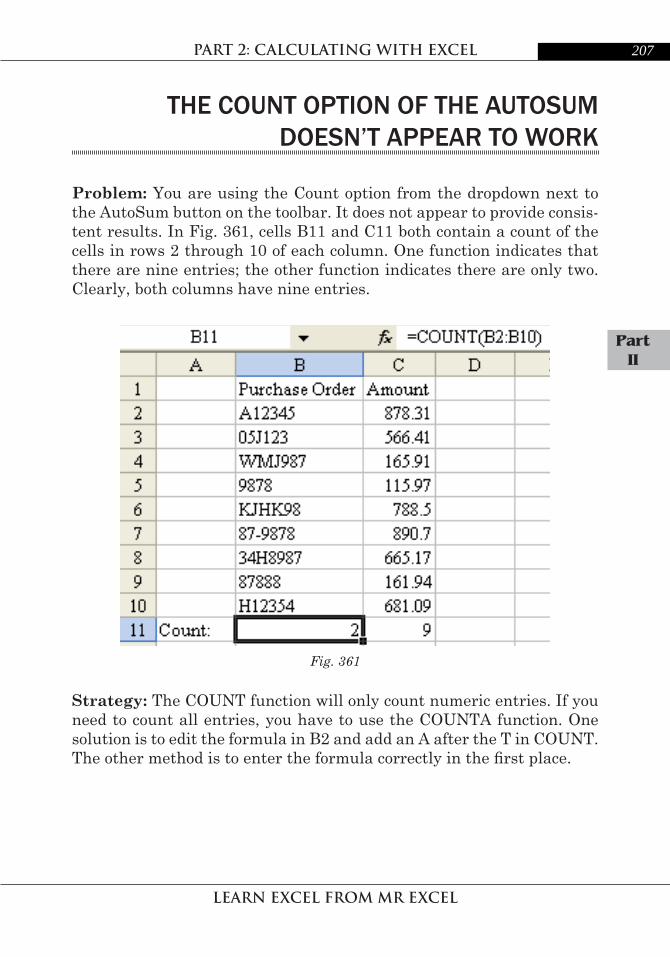
Problem: You are using the Count option from the dropdown next to the AutoSum button on the toolbar. It does not appear to provide consis-tent results. In Fig. 361, cells B11 and C11 both contain a count of the cells in rows 2 through 10 of each column. One function indicates that there are nine entries; the other function indicates there are only two. Clearly, both columns have nine entries.
Strategy: The COUNT function will only count numeric entries. If you need to count all entries, you have to use the COUNTA function. One solution is to edit the formula in B2 and add an A after the T in COUNT. The other method is to enter the formula correctly in the first place.
Fig. 361
207

Part 2: calculating with excel
learn excel From mr excel
Part 2: calculating with excel
learn excel From mr excel
1) Put the cell pointer in B11. Choose the dropdown arrow next to the AutoSum button. From the list, select More Functions…, as shown in Fig. 362.
2) There are hundreds of functions available. You can never remem-ber if COUNTA is in the Math & Trig section or somewhere else. Type the word “count” in the search box and choose Go, as shown in Fig. 363.
Excel will return a list of all functions related to the COUNT func-tion. A description of the selected function appears below the list, as shown in Fig. 364.
Fig. 362
Fig. 363
208

Part 2: calculating with excel
learn excel From mr excel
PartII
Part 2: calculating with excel
learn excel From mr excel
3) You might need to scroll through the list to find the COUNTA func-tion. As shown in Fig. 365, when you find COUNTA, choose OK.
Fig. 364
Fig. 365
209

Part 2: calculating with excel
learn excel From mr excel
Part 2: calculating with excel
learn excel From mr excel
You will now see the Function Arguments dialog box. Excel has ana-lyzed your data and predicted the range that you want to use. How-ever, Excel is not good at predicting data when the range contains numeric and alphanumeric entries. In this particular case, as shown in Fig. 366, Excel assumes we only want to COUNTA the range B9:B10.
4) If you can see the data on the worksheet, use the mouse and high-light the correct range, as shown in Fig. 367.
Fig. 366
Fig. 367
210

Part 2: calculating with excel
learn excel From mr excel
PartII
Part 2: calculating with excel
learn excel From mr excel
5) Release the mouse. Choose OK in the function arguments dialog to accept the formula.
Result: As shown in Fig. 368, the COUNTA function returns the proper value.
Summary: The COUNT function does not count text entries in a list. Use the COUNTA function instead. Functions Discussed: =COUNT(); =COUNTA()
Fig. 368
211