Embed Size (px)
Citation preview

1
Learning a Hierarchical Compositional ShapeVocabulary for Multi-class Object Representation
Sanja Fidler, Member, IEEE, Marko Boben, and Ales Leonardis, Member, IEEE
Abstract—Hierarchies allow feature sharing between objects at multiple levels of representation, can code exponential variability ina very compact way and enable fast inference. This makes them potentially suitable for learning and recognizing a higher number ofobject classes. However, the success of the hierarchical approaches so far has been hindered by the use of hand-crafted features orpredetermined grouping rules. This paper presents a novel framework for learning a hierarchical compositional shape vocabulary forrepresenting multiple object classes. The approach takes simple contour fragments and learns their frequent spatial configurations.These are recursively combined into increasingly more complex and class-specific shape compositions, each exerting a high degree ofshape variability. At the top-level of the vocabulary, the compositions are sufficiently large and complex to represent the whole shapesof the objects. We learn the vocabulary layer after layer, by gradually increasing the size of the window of analysis and reducing thespatial resolution at which the shape configurations are learned. The lower layers are learned jointly on images of all classes, whereasthe higher layers of the vocabulary are learned incrementally, by presenting the algorithm with one object class after another. Theexperimental results show that the learned multi-class object representation scales favorably with the number of object classes andachieves a state-of-the-art detection performance at both, faster inference as well as shorter training times.
Index Terms—Hierarchical representations, compositional hierarchies, unsupervised hierarchical structure learning, multiple objectclass recognition and detection, modeling object structure.
F
1 INTRODUCTION
V ISUAL categorization of objects has been an areaof active research in the vision community for
decades. Ultimately, the goal is to recognize and de-tect an increasing number of object classes in imageswithin an acceptable time frame. The problem entanglesthree highly interconnected issues: the internal objectrepresentation which should compactly capture the highvisual variability of objects and generalize well over eachclass, means of learning the representation from a setof images with as little supervision as possible, and aneffective inference algorithm that robustly matches theobject representation against the image.
Using vocabularies of visual features has been a pop-ular choice of object class representation and has yieldedsome of the most successful performances for objectdetection to date [1], [2], [3], [4], [5], [6]. However, themajority of these works are currently using flat codingschemes where each object is represented with either nostructure at all by using a bag-of-words model or onlysimple geometry induced over a set of intermediatelycomplex object parts. In this paper, our aim is to modelthe hierarchical compositional structure of the objects anddo so for multiple object classes.
Modeling structure (geometry of objects) is importantfor several reasons. Firstly, since objects within a classhave usually distinctive and similar shape, it allows for
• S. Fidler is with University of Toronto, Canada, M. Boben and A.Leonardis are with University of Ljubljana, Slovenia. A. Leonardis is alsoaffiliated with University of Birmingham, UK.E-mail: [email protected], marko.boben,[email protected]
an efficient shape parametrization with good general-ization capabilities. It further enables us to parse objectsinto meaningful components which is of particular im-portance in robotic applications where the task is notonly to detect objects but also to execute higher-levelcognitive tasks (manipulations, grasping, etc). Thirdly,by inducing the structure over the features the represen-tation becomes more robust to background clutter.
Hierarchies incorporate structural dependenciesamong the features at multiple levels: objects aredefined in terms of parts, which are further composedfrom a set of simpler constituents, etc [7], [8], [9],[10], [11], [12], [13]. Such architectures allow sharingof features between the visually similar as well asdissimilar classes at multiple levels of specificity [14],[11], [15], [12], [16]. Sharing of features means sharingcommon computations and increasing the speed of thejoint detector [2]. More importantly, shared features leadto better generalization [2] and can play an importantrole of regularization in learning of novel classes withfew training examples. Furthermore, since each featurein the hierarchy recursively models certain varianceover its parts, it captures a high structural variabilityand consequently a smaller number of features areneeded to represent each class.
Learning of feature vocabularies without or with littlesupervision is of primary importance in multi-class ob-ject representation. By learning, we minimize the amountof time of human involvement in object labeling [10],[17] and avoid bias of pre-determined grouping rules ormanually crafted features [18], [19], [20], [21]. Second,learning the representation statistically yields features
arX
iv:1
408.
5516
v1 [
cs.C
V]
23
Aug
201
4
2
most shareable between the classes, which may notbe well predicted by human labelers [22]. However,the complexity of learning the structure of a hierarchicalrepresentation bottom-up and without supervision isenormous: there is a huge number of possible featurecombinations, the number of which exponentially in-creases with each additional layer — thus an effectivelearning algorithm must be employed.
In this paper, the idea is to represent the objects with alearned hierarchical compositional shape vocabulary that hasthe following architecture. The vocabulary at each layercontains a set of hierarchical deformable models whichwe will call compositions. Each composition is definedrecursively: it is a hierarchical generative probabilisticmodel that represents a geometric configuration of asmall number of parts which are themselves hierarchicaldeformable models, i.e., compositions from a previouslayer of the vocabulary. We present a framework forlearning such a representation for multiple object classes.Learning is statistical and is performed bottom-up. Theapproach takes simple oriented contour fragments andlearns their frequent spatial configurations. These arerecursively combined into increasingly more complexand class-specific shape compositions, each exerting ahigh degree of shape variability. In the top-level of thevocabulary, the compositions are sufficiently large andcomplex to represent the whole shapes of the objects.We learn the vocabulary layer after layer, by graduallyincreasing the size of the window of analysis and thespatial resolution at which the shape configurations arelearned. The lower layers are learned jointly on images ofall classes, whereas the higher layers of the vocabularyare learned incrementally, by presenting the algorithmwith one object class after another. We assume supervi-sion in terms of a positive and a validation set of classimages — however, the structure of the vocabulary islearned in an unsupervised manner. That is, the numberof compositions at each layer, the number of parts foreach of the compositions along with the distribution pa-rameters are inferred from the data without supervision.
We experimentally demonstrate several important is-sues: 1.) Applied to a collection of natural images, theapproach learns hierarchical models for various curva-tures, T- and L- junctions, i.e., features usually empha-sized by the Gestalt theory [23]; 2.) We show that thesegeneric compositions can be effectively used for objectclassification; 3.) For object detection we demonstratea competitive speed of detection with respect to therelated approaches already for a single class. 4.) Formulti-class object detection we achieve a highly sub-linear growth in the size of the hierarchical vocabulary atmultiple layers and, consequently, a scalable complexityof inference as the number of modeled classes increases;5.) We demonstrate a competitive detection accuracywith respect to the current state-of-the-art. Furthermore,the learned representation is very compact — a hierarchymodeling 15 object classes uses only 1.6Mb on disk.
The remainder of this paper is organized as follows.
In Sec. 2 we review the related work. Sec. 3 presentsour hierarchical compositional representation of objectshape with recognition and detection described in Sec. 4.In Sec. 5 our learning framework is proposed. Theexperimental results are presented in Sec. 6. The paperconcludes with a summary and discussion in Sec. 7 andpointers to future work in Sec. 8.
2 RELATED WORK AND CONTRIBUTIONS
Compositional hierarchies. Several compositional ap-proaches to modeling objects have been proposed inthe literature, however, most of them relied on hand-crafted representations, pre-determined grouping rulesor supervised training with manually annotated objectparts [10], [19], [20], [24]. The reader is referred to [10],[25] for a thorough review.
Unsupervised learning of hierarchical compositionalvocabularies. Work on unsupervised hierarchical learninghas been relatively scarce. Utans [26] has been the firstto address unsupervised learning of compositional rep-resentations. The approach learned hierarchical mixturemodels of feature combinations, and was utilized onlearning simple dot patterns.
Based on the Fukushima’s model [27], Riesenhuberand Poggio [28] introduced the HMAX approach whichrepresents objects with a 2-layer hierarchy of Gaborfeature combinations. The original HMAX used a vo-cabulary of pre-determined features, while these havesubsequently been replaced with randomly chosen tem-plates [29]. Since no statistical learning is involved, asmuch as several thousands of features are needed to rep-resent the objects. An improved learning algorithm hasrecently been proposed by Masquelier and Thorpe [30].
Among the neural network representatives, Convo-lutional nets [31], [32] have been most widely andsuccessfully applied to generic object recognition. Theapproach builds a hierarchical feature extraction andclassification system with fast feed-forward processing.The hierarchy stacks one or several feature extractionstages, each of which consists of filter bank layer, non-linear transformation layers, and a pooling layer thatcombines filter responses over local neighborhoods us-ing an average or max operation, thereby achievinginvariance to small distortions [32]. A similar approachis proposed by Hinton [33] with recent improvementsby Ng et al. [34]. One of the main drawbacks of theseapproaches, however, may be that they do not explicitlymodel the spatial relations among the features and arethus potentially less robust to shape variations.
Bouchard and Triggs [7] proposed a 3−layer hierarchy(extension of the constellation model [1]) and a similarrepresentation was proposed by Torralba et al. [2], [35].For tractability, all of these models are forced to usevery sparse image information, where prior to learningand detection, a small number (around 30) of interestpoints are detected. Using highly discriminative SIFTfeatures might limit their success in cluttered images or

3
on structurally simpler objects with little texture. Therepeatability of the SIFT features across the classes isalso questionable [29]. On the other hand, our approachis capable of dealing with several tens of thousands ofcontour fragments as input. We believe that the use ofrepeatable, dense and indistinctive contour fragmentsprovide us with a higher repeatability of the subsequentobject representation facilitating a better performance.
Epshtein and Ullman [36] approached the represen-tation from the opposite end; the hierarchy is built bydecomposing object relevant image patches into recur-sively smaller entities. The approach has been utilized onlearning each class individually while a joint multi-classrepresentation has not been pursued. A similar line ofwork was adopted by Mikolajczyk et al. [37] and appliedto recognize and detect multiple (5) object classes.
Todorovic and Ahuja [38] proposed a data-drivenapproach where a hierarchy for each object example isgenerated automatically by a segmentation algorithm.The largest repeatable subgraphs are learned to repre-sent the objects. Since bottom-up processes are usuallyunstable, exhaustive grouping is employed which resultsin long training and inference times.
Ommer and Buhmann [12] proposed an unsupervisedhierarchical learning approach, which has been success-fully utilized for object classification. The features at eachlayer are defined as histograms over a larger, spatiallyconstrained area. Our approach explicitly models thespatial relations among the features, which should al-low for a more reliable detection of objects with lowersensitivity to background clutter.
The learning frameworks most related to ours includethe work by [39], [40] and just recently [41]. However,all of these methods build separate hierarchies for eachobject class. This, on the one hand, avoids the massivenumber of possible feature combinations present in di-verse objects, but, on the downside, does not exploit theshareability of features among the classes.
Our approach is also related to the work on multi-classshape recognition by Amit et al. [42], [43], [15], and someof their ideas have also inspired our approach. Whilethe conceptual representation is similar to ours, thecompositions there are designed by hand, the hierarchyhas only three layers (edges, parts and objects), and theapplication is mostly targeted to reading licence plates.
While surely equally important, the work on learningof visual taxonomies [44], [45] of object classes tacklesthe categorization/recognition process by hierarchicalcascade of classifiers. Our hierarchy is compositional andgenerative with respect to object structure and does notaddress the taxonomic organization of object classes. Weproposed a model that is hierarchical both in structureas well as classes (taxonomy) in our later work [46].
Our approach is also related to the discriminativelytrained grammars by Girshick et al. [13], developed afterour original work was published. Like us, this approachmodels objects with deformable parts and subparts, theweights of which are trained using structure prediction.
This approach has achieved impressive results for objectdetection in the past years. Its main drawback, however,is that the structure of the grammar needs to be specifiedby hand which is what we want to avoid doing here.
Compositional representations are currently not atthe level of performance of supervised deep convolu-tional networks [47] which discriminatively train mil-lions of weights (roughly three orders of magnitudemore weights than our approach). To perform well thesenetworks typically need millions of training examples,which is three or four orders of magnitude more than ourapproach. While originally designed for classificationthese networks have recently been very successful inobject detection when combined with bottom-up regionproposals [48]. We believe that these type of networkscan also benefit from the ideas presented here.
Contour-based recognition approaches. Since our ap-proach deals with object shape, we also briefly reviewthe related work on contour-based object class detection.
Contour fragments have been employed in the earlierwork by Selinger and Nelson [49] and a number offollow-up works have used a similar approach. Opeltet al. [3] learned boundary fragments in a boosting frame-work and used them in a Hough voting scheme for ob-ject class detection. Ferrari et al. [50], [5] extracted kPASfeatures which were learned by combining k roughlystraight contour fragments. The learned kPAS featuresresemble those obtained in the lower hierarchical layersby our approach. Fergus et al. [51], [1] represent objectsas constellations of object parts and propose an approachthat learns the model from images without supervisionand in a scale invariant manner. The part-based repre-sentation is similar to ours, however in contrast, ourapproach learns a hierarchical part-based representation.
To the best of our knowledge, we are the first to1.) learn generic shape structures from images at mul-tiple hierarchical layers and without supervision, which,interestingly, resemble those predicted by the Gestalttheory [23], 2.) learn a multi-class generative composi-tional representation in a bottom-up manner from simplecontour fragments, 3.) demonstrate scalability of a hier-archical generative approach when the number of classesincreases — in terms of the speed of inference, storage,and training times.
This article conjoins and extends several of our con-ference papers on learning of a hierarchical composi-tional vocabulary of object shape [52], [11], [53], [54].Specifically, the original model has been reformulatedand more details have been included which could not begiven in the conference papers due to page constraints.Further, more classes have been used in the experiments,the approach has been tested on several standard recog-nition benchmarks and an analysis with respect to thecomputational behavior of the proposed approach hasbeen carried out.

4
Fig. 1. Left: Illustration of the hierarchical vocabulary. Theshapes depict the compositions ω` and the links between themdenote the compositional relations between them. Note thatthere are no actual images stored in the vocabulary – thedepicted shapes are mean shapes represented by the composi-tions. Right: An example of a complete composition model fromlayer 3. The blue patches are the limiting sizes within which themodel can generate shapes, while the red ellipses denote theGaussians representing the spatial relations between the parts.
3 A HIERARCHICAL COMPOSITIONAL OBJECTREPRESENTATION
The complete hierarchical framework addresses threemajor issues: the representation, inference and learning.In this Section we present our hierarchical compositionalobject representation.
Our aim is to model the distribution of object shapesin a given class and we wish to do so for multiple objectclasses in a computationally efficient way. The idea isto represent the objects with a single learned hierarchicalcompositional shape vocabulary that has the following ar-chitecture. The vocabulary at each layer contains a setof hierarchical deformable models which we will callcompositions. Each composition is defined recursively: itrepresents a geometric configuration of a small numberof parts which are compositions from the previous layerof the vocabulary. Different compositions can share mod-els for the parts, which makes the vocabulary efficient insize and results in faster inference.
The geometric configuration of parts is modeled byrelative spatial relations between each of the parts andone part called a reference part. The hierarchical “topol-ogy” of a composition is assumed to be a tree and islearned in a way to ensure that its (sub)parts do notoverlap or overlap minimally.
Note that a particular shape can be composed inmultiple different ways, e.g. a rectangle can be formed bytwo sets of parallel lines or four properly aligned rightangles. Thus some of the compositions may describe thesame shape but have very different topologies (different
tree structures). To deal with this issue, such composi-tions are grouped into OR nodes which act as mixturemodels (similarly as in [55]). This is done based on thegeometric similarity of the shape they represent.
The structure of the compositions will be learned in anunsupervised manner from images, along with the corre-sponding parameters. The number of compositions thatmake a particular layer in the vocabulary will also not beset in advance but determined through learning. We willlearn the layers 2 and 3 without any supervision, from apool of unlabeled images. To learn the higher layers, wewill assume bounding boxes with object labels, i.e., theset of positive and validation boxes of objects for eachclass needs to be given. The amount of supervision theapproach needs is further discussed in Sec. 5.2.
At the lowest (first) layer, the hierarchical vocabularyconsists of a small number of base models that representshort contour fragments at coarsely defined orientations.The number of orientations is assumed given. At the top-most layer the compositions will represent the shapes ofthe whole objects. For a particular object class, a numberof top-layer compositions will be used to represent thewhole distribution of shapes in the class, i.e., each top-layer composition will model a certain aspect (3D viewor an articulation) of the objects within the class. The leftside of Fig. 1 illustrates the representation.
Due to the recursive definition, a composition at anylayer of the vocabulary is thus an “autonomous” de-formable model. As such, a composition at the top layercan act as a detector for an object class, while a com-position at an intermediate layer acts as a detector fora less complex shape (for example, an L junction). Sincewe are combining deformable models as we go up in thehierarchy, we are capturing an increasing variability intothe representation while at the same time preserving thespatial arrangements of the shape components.
We will use the following notation. Let Ω denote theset and structure of all compositions in the vocabularyand Θ their parameters. Since the vocabulary has ahierarchical structure we will write it as Ω = Ω1 ∪Ω1 ∪ Ω2 ∪ Ω2 ∪ · · · ∪ ΩO ∪ ΩC where Ω` = ω`ii isa set of compositions at layer ` and Ω` = ω`ii is aset of OR-compositions from layer `, more specifically,ω`i ⊆ Ω`. Whenever it is clear from the context, we willomit the index i. With ΩO we denote the top, objectlayer of compositions (we will use O = 6 in this paper,and this choice is discussed in Sec. 5.2), which roughlycode the whole shapes of the objects. The final, classlayer ΩC , is an OR layer of object layer compositions(ΩO), i.e., each class layer composition pools all of thecorresponding object layer compositions from ΩO foreach class separately.
The definition of a composition with respect to justone layer below is similar to that of the constellationmodel [51]. A composition ω`, where ` > 1, consists of Pparts (P can differ across compositions), with appearancesθa
` = [θa`j ]Pj=1 and geometric parameters θg
` = [θg`j ]Pj=1.
The parts are compositions from the previous OR layer
5
Ω`−1. One of the parts that forms ω` is taken as areference and the positions of other parts are definedrelative to its position. We will refer to such a part as areference part.
The appearance θa`j is an N `−1 dimensional vector,
where N `−1 = |Ω`−1| is the number of OR-compositionsat layer ` − 1, and θa
`j(k) represents the compatibility
between ω`−1k and j-th part of ω`. This vector will be
sparse, thus only the non-zero entries need to be kept.For example, imagine composing an object model for theclass car. A car can have many different shapes for thetrunk or the front of the car. Thus a car detector should“fire” if any part that looks like any of the trunks ispresent in the rear location and any front part in the frontlocation of the detector. We allow θa
`j to have multiple
positive entries only at the object level ΩO, for otherlayers we consider θa `j to be non-zero only at one entry(in this case, equal to 1).
The geometric relations between the position of eachof the parts relative to the reference part are modeledby two-dimensional Gaussians θg
`j = (µ`j ,Σ
`j). For the
convenience of notation later on, we will also representthe location of a reference part with respect to itself witha Gaussian having zero mean and small variance, ε2Id.
We allow for a composition to also have “repulsive”parts. These are the parts that the composition cannotconsist of. For example, a handle is a repulsive partfor a cup since its presence indicates the class mug. Weintroduce the repulsive parts to deal with compositionsthat are supersets of one another.
The models at the first layer of the vocabulary aredefined over the space of image features, which willin this paper be n-dimensional Gabor feature vectors(explained in Sec. 4.1).
Note that each composition can only model shapeswithin a limited spatial extent, that is, the windowaround a modeled shape is of limited size and the sizeis the same for all compositions at a particular layer `of the vocabulary. We will denote it with r`. The size r`
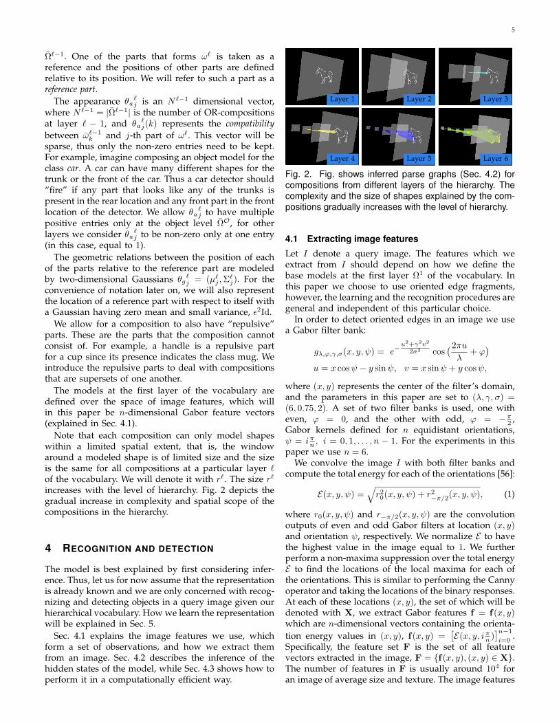
increases with the level of hierarchy. Fig. 2 depicts thegradual increase in complexity and spatial scope of thecompositions in the hierarchy.
4 RECOGNITION AND DETECTION
The model is best explained by first considering infer-ence. Thus, let us for now assume that the representationis already known and we are only concerned with recog-nizing and detecting objects in a query image given ourhierarchical vocabulary. How we learn the representationwill be explained in Sec. 5.
Sec. 4.1 explains the image features we use, whichform a set of observations, and how we extract themfrom an image. Sec. 4.2 describes the inference of thehidden states of the model, while Sec. 4.3 shows how toperform it in a computationally efficient way.
Layer 1 Layer 2 Layer 3
Layer 4 Layer 5 Layer 6
Fig. 2. Fig. shows inferred parse graphs (Sec. 4.2) forcompositions from different layers of the hierarchy. Thecomplexity and the size of shapes explained by the com-positions gradually increases with the level of hierarchy.
4.1 Extracting image features
Let I denote a query image. The features which weextract from I should depend on how we define thebase models at the first layer Ω1 of the vocabulary. Inthis paper we choose to use oriented edge fragments,however, the learning and the recognition procedures aregeneral and independent of this particular choice.
In order to detect oriented edges in an image we usea Gabor filter bank:
gλ,ϕ,γ,σ(x, y, ψ) = e−u2+γ2v2
2σ2 cos(2πu
λ+ ϕ
)u = x cosψ − y sinψ, v = x sinψ + y cosψ,
where (x, y) represents the center of the filter’s domain,and the parameters in this paper are set to (λ, γ, σ) =(6, 0.75, 2). A set of two filter banks is used, one witheven, ϕ = 0, and the other with odd, ϕ = −π2 ,Gabor kernels defined for n equidistant orientations,ψ = iπn , i = 0, 1, . . . , n − 1. For the experiments in thispaper we use n = 6.
We convolve the image I with both filter banks andcompute the total energy for each of the orientations [56]:
E(x, y, ψ) =√r20(x, y, ψ) + r2
−π/2(x, y, ψ), (1)
where r0(x, y, ψ) and r−π/2(x, y, ψ) are the convolutionoutputs of even and odd Gabor filters at location (x, y)and orientation ψ, respectively. We normalize E to havethe highest value in the image equal to 1. We furtherperform a non-maxima suppression over the total energyE to find the locations of the local maxima for each ofthe orientations. This is similar to performing the Cannyoperator and taking the locations of the binary responses.At each of these locations (x, y), the set of which will bedenoted with X, we extract Gabor features f = f(x, y)which are n-dimensional vectors containing the orienta-tion energy values in (x, y), f(x, y) =
[E(x, y, iπn )
]n−1
i=0.
Specifically, the feature set F is the set of all featurevectors extracted in the image, F = f(x, y), (x, y) ∈ X.The number of features in F is usually around 104 foran image of average size and texture. The image features
6
orient. 1orient. 2orient. 3orient. 4orient. 5orient. 6
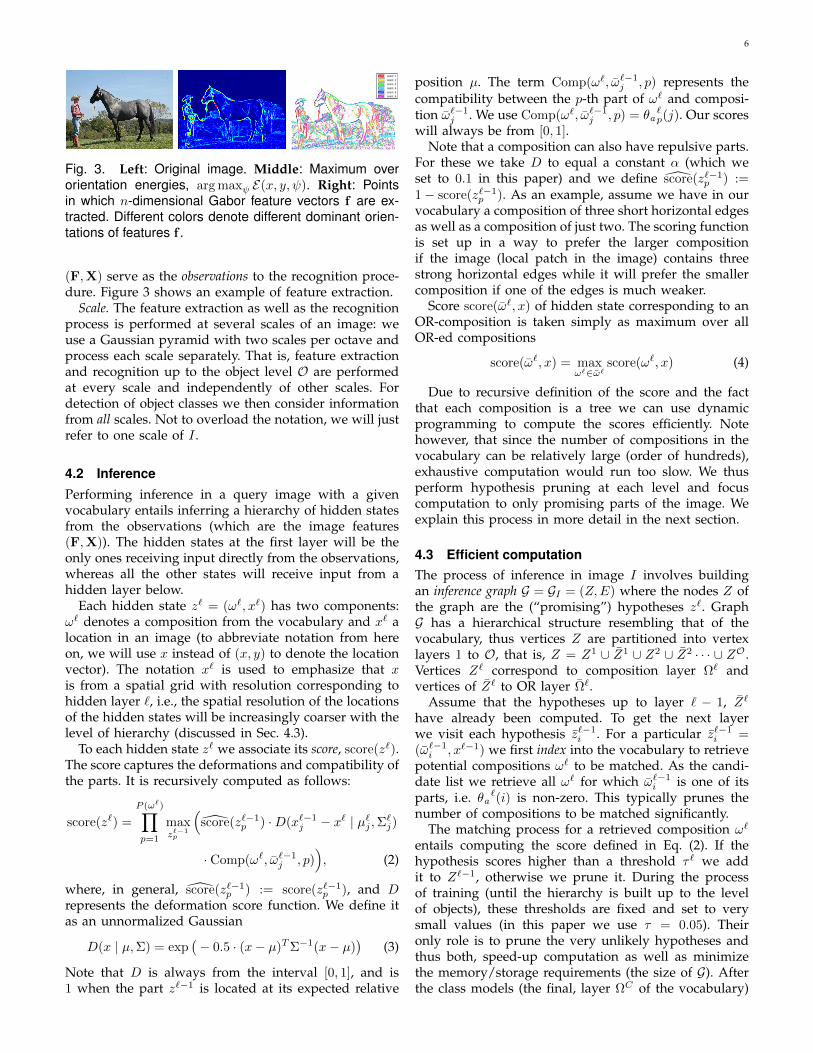
Fig. 3. Left: Original image. Middle: Maximum overorientation energies, arg maxψ E(x, y, ψ). Right: Pointsin which n-dimensional Gabor feature vectors f are ex-tracted. Different colors denote different dominant orien-tations of features f .
(F,X) serve as the observations to the recognition proce-dure. Figure 3 shows an example of feature extraction.
Scale. The feature extraction as well as the recognitionprocess is performed at several scales of an image: weuse a Gaussian pyramid with two scales per octave andprocess each scale separately. That is, feature extractionand recognition up to the object level O are performedat every scale and independently of other scales. Fordetection of object classes we then consider informationfrom all scales. Not to overload the notation, we will justrefer to one scale of I .
4.2 InferencePerforming inference in a query image with a givenvocabulary entails inferring a hierarchy of hidden statesfrom the observations (which are the image features(F,X)). The hidden states at the first layer will be theonly ones receiving input directly from the observations,whereas all the other states will receive input from ahidden layer below.
Each hidden state z` = (ω`, x`) has two components:ω` denotes a composition from the vocabulary and x` alocation in an image (to abbreviate notation from hereon, we will use x instead of (x, y) to denote the locationvector). The notation x` is used to emphasize that xis from a spatial grid with resolution corresponding tohidden layer `, i.e., the spatial resolution of the locationsof the hidden states will be increasingly coarser with thelevel of hierarchy (discussed in Sec. 4.3).
To each hidden state z` we associate its score, score(z`).The score captures the deformations and compatibility ofthe parts. It is recursively computed as follows:
score(z`) =
P (ω`)∏p=1
maxz`−1p
(score(z`−1
p ) ·D(x`−1j − x` | µ`j ,Σ`j)
· Comp(ω`, ω`−1j , p)
), (2)
where, in general, score(z`−1p ) := score(z`−1
p ), and Drepresents the deformation score function. We define itas an unnormalized Gaussian
D(x | µ,Σ) = exp(− 0.5 · (x− µ)TΣ−1(x− µ)
)(3)
Note that D is always from the interval [0, 1], and is1 when the part z`−1 is located at its expected relative
position µ. The term Comp(ω`, ω`−1j , p) represents the
compatibility between the p-th part of ω` and composi-tion ω`−1
j . We use Comp(ω`, ω`−1j , p) = θa
`p(j). Our scores
will always be from [0, 1].Note that a composition can also have repulsive parts.
For these we take D to equal a constant α (which weset to 0.1 in this paper) and we define score(z`−1
p ) :=1− score(z`−1
p ). As an example, assume we have in ourvocabulary a composition of three short horizontal edgesas well as a composition of just two. The scoring functionis set up in a way to prefer the larger compositionif the image (local patch in the image) contains threestrong horizontal edges while it will prefer the smallercomposition if one of the edges is much weaker.
Score score(ω`, x) of hidden state corresponding to anOR-composition is taken simply as maximum over allOR-ed compositions
score(ω`, x) = maxω`∈ω`
score(ω`, x) (4)
Due to recursive definition of the score and the factthat each composition is a tree we can use dynamicprogramming to compute the scores efficiently. Notehowever, that since the number of compositions in thevocabulary can be relatively large (order of hundreds),exhaustive computation would run too slow. We thusperform hypothesis pruning at each level and focuscomputation to only promising parts of the image. Weexplain this process in more detail in the next section.
4.3 Efficient computationThe process of inference in image I involves buildingan inference graph G = GI = (Z,E) where the nodes Z ofthe graph are the (“promising”) hypotheses z`. GraphG has a hierarchical structure resembling that of thevocabulary, thus vertices Z are partitioned into vertexlayers 1 to O, that is, Z = Z1 ∪ Z1 ∪ Z2 ∪ Z2 · · · ∪ ZO.Vertices Z` correspond to composition layer Ω` andvertices of Z` to OR layer Ω`.
Assume that the hypotheses up to layer ` − 1, Z`
have already been computed. To get the next layerwe visit each hypothesis z`−1
i . For a particular z`−1i =
(ω`−1i , x`−1) we first index into the vocabulary to retrieve
potential compositions ω` to be matched. As the candi-date list we retrieve all ω` for which ω`−1
i is one of itsparts, i.e. θa `(i) is non-zero. This typically prunes thenumber of compositions to be matched significantly.
The matching process for a retrieved composition ω`
entails computing the score defined in Eq. (2). If thehypothesis scores higher than a threshold τ ` we addit to Z`−1, otherwise we prune it. During the processof training (until the hierarchy is built up to the levelof objects), these thresholds are fixed and set to verysmall values (in this paper we use τ = 0.05). Theironly role is to prune the very unlikely hypotheses andthus both, speed-up computation as well as minimizethe memory/storage requirements (the size of G). Afterthe class models (the final, layer ΩC of the vocabulary)

7
are learned we can also learn the thresholds in a wayto optimize the speed of inference while retaining thedetection accuracy, as will be explained in Sec. 5.2.1.Note that due to the thresholds, we can avoid some ofthe computation: we do not need to consider the spatiallocations of parts that are outside the τ ` Gaussian radius.
Reduction in spatial resolution. After each layer Z` isbuilt, we perform spatial downsampling, where the lo-cations x` of the hidden states z` are downsampledby a factor ρ` < 1. Among the states that code thesame composition ω` and for which the locations (takento have integer values) become equal, only the statewith the highest score is kept. We use ρ1 = 1 andρ` = 0.5, ` > 1. This step is mainly meant to reduce thecomputational load: by reducing the spatial resolution ateach layer, we bring the far-away (location-wise) hiddenstates closer. This, indirectly, keeps the scales of theGaussians relatively small across all compositions in thevocabulary and makes inference faster.
The OR layer Z` pools all compositions z` = (ω`, x`) ∈Z` for which z` = (ω`, x`) : ω` ∈ ω` into one node,which further reduces the hypotheses space.
Edges of G connect vertices of Z` to vertices of Z`−1
and vertices of Z` to vertices of Z`. Each z` = (ω`, x`) isconnected to vertices z`−1
p that yield the max score for thepart j in Eq. (2) and each vertex z` = (ω`, x`) connectsto z` giving the max value in Eq. (4). The subgraph of Gon vertices reachable from vertex z via downward edgepaths is called a parse graph and denoted by P(z). A setof vertices of P(z) from Z1, i.e. layer 1 vertices reachablefrom z through edges in G, are called support of z anddenoted with supp(z). See Fig. 2 for examples of parsegraphs and supports of vertices from different layers.The definition of support is naturally extended to a setof nodes as supp(S) = ∪z∈S supp(z).
5 LEARNING
This section addresses the problem of learning the rep-resentation, which entails the following:
1) Learning the vocabulary of compositions. Findingan appropriate set of compositions to represent ourdata, learning the structure of compositions (thenumber of parts and a (rough) initialization of theparameters) and learning the OR-compositions.
2) Learning the parameters of the representation.Finding the parameters for spatial relations andappearance for each composition as well as thethresholds to be used in the approximate inferencealgorithm.
In the learning process our aim is to build a vocabularyof compositions which tries to meet the following twoconditions: (a) Detections of compositions on the objectlayer, ΩO, give good performance on the train/validationset. (b) The vocabulary is minimal, optimizing the in-ference time. Intuitively, it is possible to build a goodcomposition on the object layer if the previous layerΩO−1 produces a good “coverage” of training examples.
By coverage we mean that the supports of hypothesesin ZO−1 contain most of the feature locations X. Hence,we would like to build our vocabulary such that thecompositions at each layer cover the feature location Xin the training set sufficiently well and is, according to(b), the most compact representation.
To find a good vocabulary according to the aboveconstraints is a hard problem. Our strategy is to learn onelayer at a time, in a bottom up fashion, and at each layerlearn a small compact vocabulary while maintaining itsgood coverage ratio. Bottom-up layer learning is alsothe main strategy adopted to learn the convolutionalnetworks [31], [33].
We emphasize that our learning algorithm uses severalheuristics and is not guaranteed to find the optimalvocabulary. Deriving a more mathematically elegantlearning approach is part of our future work.
5.1 Learning the structure
Here we explain how we learn the initial set of composi-tions, their structure and initial values of the parameters(which are re-estimated as described in Sec. 5.1.4).
The first layer, ` = 1, is fixed thus the first layer that welearn is ` = 2. Since learning the vocabulary is recursivewe will describe how to learn layer ` from ` − 1. Wewill assume that for each training image I we have theinference graph GI = (Z,E) built up to layer `−1, whichis obtained as described in Sec. 4.2.
Define a spatial neighborhood of radius r` around thenode z`−1 = (ω`−1, x`−1) with N (z`−1). We also definethe support of N (z`−1) by re-projecting the circular areato the original image resolution and finding all imagefeatures whose locations fall inside the projected circulararea. Our goal in learning is to find a vocabulary thatbest explains all of the spatial neighborhoods N (z`−1),where z`−1 ∈ Z`−1:
Ω`∗ = arg maxΩ`
(− C
∑ω`
i∈Ω`
P (ω`i )+ (5)
+∑Ij
∑k | z`−1
k ∈Z`−1Ij
score(N (z`−1k ),Ω`)
)
Here P (ω`i ) is the number of parts that defines acomposition ω`i , and C is a weight that balances the twoterms. We define the score term as follows:
score(N (z`−1k ),Ω`) = max
z`
(scorecoverage(N (z`−1
k ), z`) +
(6)
scoretree(z`)),
where
scorecoverage(N (z`−1k ), z`) =
| supp(z`) ∩ supp(N (z`−1k ))|
| supp(z`) ∪ supp(N (z`−1k ))|
(7)
8
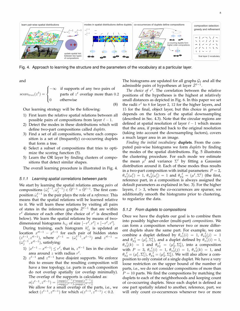
learn pair-wise spatial distributions
update spatial hist.between two typesof compositions
modes in spatial distributions define duplets
co-ocurring duplets formhigher order compositions
co-occurrences of duplets define compositions composition selection:
greedy and refinement
final layer 2 vocabulary
Fig. 4. Approach to learning the structure and the parameters of the vocabulary at a particular layer.
and
scoretree(z`) =
−∞ if supports of any two pairs of
parts of z` overlap more than 0.2
0 otherwise(8)
Our learning strategy will be the following:1) First learn the relative spatial relations between all
possible pairs of compositions from layer `− 1.2) Detect the modes in these distributions which will
define two-part compositions called duplets.3) Find a set of all compositions, where each compo-
sition is a set of (frequently) co-occurring dupletsthat form a tree.
4) Select a subset of compositions that tries to opti-mize the scoring function (5).
5) Learn the OR layer by finding clusters of compo-sitions that detect similar shapes.
The overall learning procedure is illustrated in Fig. 4.
5.1.1 Learning spatial correlations between parts
We start by learning the spatial relations among pairs ofcompositions (ω`−1
i , ω`−1j ) ∈ Ω`−1 × Ω`−1. The first com-
position ω`−1i in the pair plays the role of a reference. This
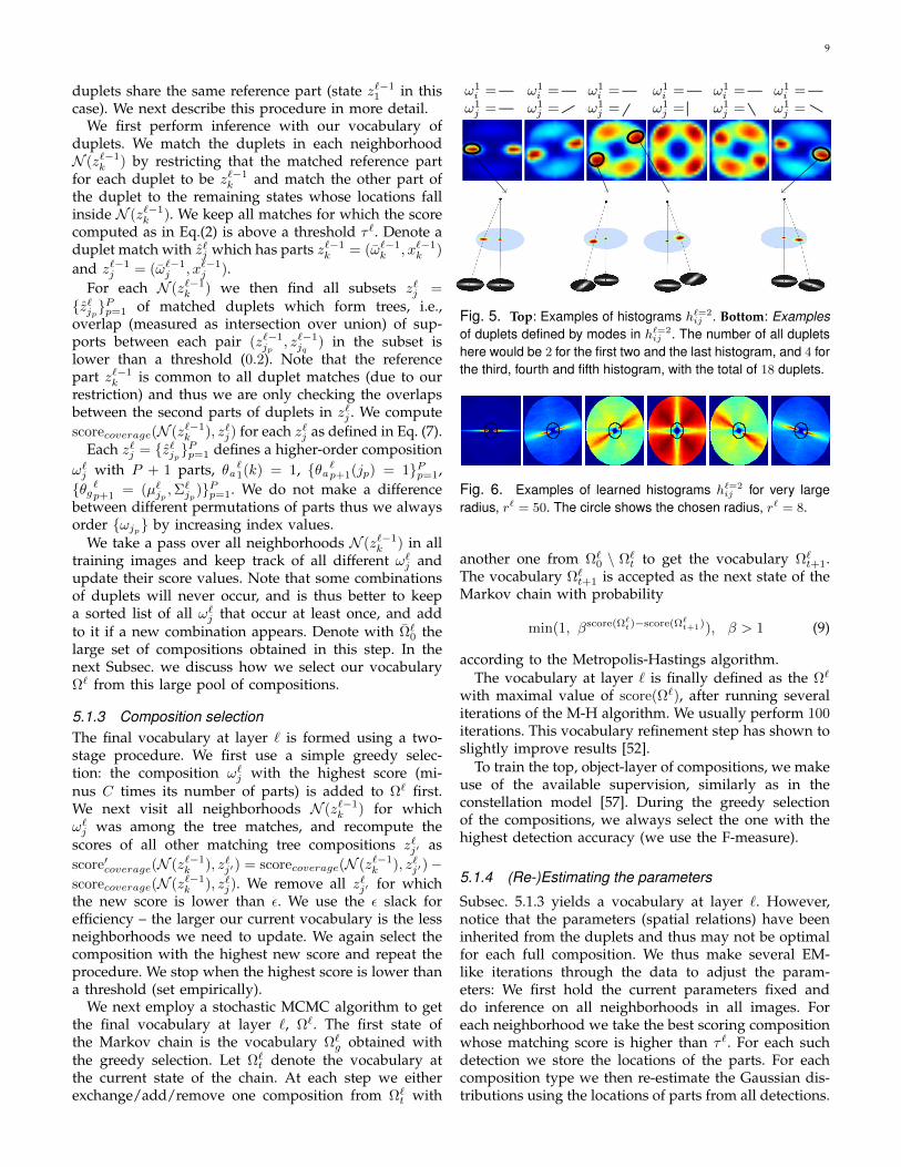
means that the spatial relations will be learned relativeto it. We will learn these relations by visiting all pairsof states in the inference graphs Z`−1 that are withinr` distance of each other (the choice of r` is describedbelow). We learn the spatial relations by means of two-dimensional histograms hij of size [−r`, r`]× [−r`, r`].
During training, each histogram h`ij is updated atlocation x′`−1 − x`−1 for each pair of hidden states(z`−1, z′`−1), where z`−1 = (ω`−1
i , x`−1) and z′`−1 =(ω`−1j , x′`−1), satisfying:
1) |x`−1 − x′`−1| ≤ r`, that is, z′`−1 lies in the circulararea around z with radius r`.
2) z`−1 and z′`−1 have disjoint supports. We enforcethis to ensure that the resulting composition willhave a tree topology, i.e. parts in each compositiondo not overlap spatially (or overlap minimally).The overlap of the supports is calculated as:o(z`−1, z′`−1) = | supp(z`−1)∩supp(z′`−1)|
| supp(z`−1)∪supp(z′`−1)|We allow for a small overlap of the parts, i.e., weselect (z`−1, z′`−1) for which o(z`−1, z′`−1) < 0.2.
The histograms are updated for all graphs GI and all theadmissible pairs of hypotheses at layer Z`−1.
The choice of r`. The correlation between the relativepositions of the hypotheses is the highest at relativelysmall distances as depicted in Fig. 6. In this paper we setthe radii r` to 8 for layer 2, 12 for the higher layers, and15 for the final, object layer, but this choice in generaldepends on the factors of the spatial downsampling(described in Sec. 4.3). Note that the circular regions aredefined at spatial resolution of layer `− 1 which meansthat the area, if projected back to the original resolution(taking into account the downsampling factors), coversa much larger area in an image.
Finding the initial vocabulary: duplets. From the com-puted pair-wise histograms we form duplets by findingthe modes of the spatial distributions. Fig. 5 illustratesthe clustering procedure. For each mode we estimatethe mean µ` and variance Σ` by fitting a Gaussiandistribution around it. Each of these modes thus resultsin a two-part composition with initial parameters: P = 2,θa`1(ω`i ) = 1, θa `2(ω`j) = 1 and θg
`2 = (µ`,Σ`) (the first,
reference part, in a composition is always assigned thedefault parameters as explained in Sec. 3). For the higherlayers, ` > 3, where the co-occurrences are sparser, weadditionally smooth the histograms prior to clustering,to regularize the data.
5.1.2 From duplets to compositions
Once we have the duplets our goal is to combine theminto possibly higher-order (multi-part) compositions. Wecan form a composition whenever two or more differ-ent duplets share the same part. For example, we cancombine a duplet defined by θa
`1(i) = 1, θa `2(j) = 1
and θg`2 = (µ`1,Σ
`1), and a duplet defined by θa
`1(i) = 1,
θa`2(k) = 1 and θg
`2 = (µ`2,Σ
`2), into a composition
with P = 3, θa `1(i) = 1, θa `2(j) = 1, θa `3(k) = 1, andθg`2 = (µ`1,Σ
`1), θg`3 = (µ`2,Σ
`2). We will also allow a com-
position to only consist of a single duplet. We have a veryloose restriction on the upper bound of the number ofparts, i.e., we do not consider compositions of more thanP = 10 parts. We find the compositions by matching theduplets to each of the neighborhoods and keeping countof co-occurring duplets. Since each duplet is defined asone part spatially related to another, reference, part, wewill only count co-occurrences whenever two or more
9
duplets share the same reference part (state z`−11 in this
case). We next describe this procedure in more detail.We first perform inference with our vocabulary of
duplets. We match the duplets in each neighborhoodN (z`−1
k ) by restricting that the matched reference partfor each duplet to be z`−1
k and match the other part ofthe duplet to the remaining states whose locations fallinside N (z`−1
k ). We keep all matches for which the scorecomputed as in Eq.(2) is above a threshold τ `. Denote aduplet match with z`j which has parts z`−1
k = (ω`−1k , x`−1
k )
and z`−1j = (ω`−1
j , x`−1j ).
For each N (z`−1k ) we then find all subsets z`j =
z`jpPp=1 of matched duplets which form trees, i.e.,
overlap (measured as intersection over union) of sup-ports between each pair (z`−1
jp, z`−1jq
) in the subset islower than a threshold (0.2). Note that the referencepart z`−1
k is common to all duplet matches (due to ourrestriction) and thus we are only checking the overlapsbetween the second parts of duplets in z`j . We computescorecoverage(N (z`−1
k ), z`j) for each z`j as defined in Eq. (7).Each z`j = z`jp
Pp=1 defines a higher-order composition
ω`j with P + 1 parts, θa `1(k) = 1, θa `p+1(jp) = 1Pp=1,θg`p+1 = (µ`jp ,Σ
`jp
)Pp=1. We do not make a differencebetween different permutations of parts thus we alwaysorder ωjp by increasing index values.
We take a pass over all neighborhoods N (z`−1k ) in all
training images and keep track of all different ω`j andupdate their score values. Note that some combinationsof duplets will never occur, and is thus better to keepa sorted list of all ω`j that occur at least once, and addto it if a new combination appears. Denote with Ω`0 thelarge set of compositions obtained in this step. In thenext Subsec. we discuss how we select our vocabularyΩ` from this large pool of compositions.
5.1.3 Composition selectionThe final vocabulary at layer ` is formed using a two-stage procedure. We first use a simple greedy selec-tion: the composition ω`j with the highest score (mi-nus C times its number of parts) is added to Ω` first.We next visit all neighborhoods N (z`−1
k ) for whichω`j was among the tree matches, and recompute thescores of all other matching tree compositions z`j′ asscore′coverage(N (z`−1
k ), z`j′) = scorecoverage(N (z`−1k ), z`j′)−
scorecoverage(N (z`−1k ), z`j). We remove all z`j′ for which
the new score is lower than ε. We use the ε slack forefficiency – the larger our current vocabulary is the lessneighborhoods we need to update. We again select thecomposition with the highest new score and repeat theprocedure. We stop when the highest score is lower thana threshold (set empirically).
We next employ a stochastic MCMC algorithm to getthe final vocabulary at layer `, Ω`. The first state ofthe Markov chain is the vocabulary Ω`g obtained withthe greedy selection. Let Ω`t denote the vocabulary atthe current state of the chain. At each step we eitherexchange/add/remove one composition from Ω`t with
ω1i = —ω1j = —
ω1i = —ω1j = —
ω1i = —ω1j = —
ω1i = —ω1j = —
ω1i = —ω1j = —
ω1i = —ω1j = —
Fig. 5. Top: Examples of histograms h`=2ij . Bottom: Examples
of duplets defined by modes in h`=2ij . The number of all duplets
here would be 2 for the first two and the last histogram, and 4 forthe third, fourth and fifth histogram, with the total of 18 duplets.
Fig. 6. Examples of learned histograms h`=2ij for very large
radius, r` = 50. The circle shows the chosen radius, r` = 8.
another one from Ω`0 \ Ω`t to get the vocabulary Ω`t+1.The vocabulary Ω`t+1 is accepted as the next state of theMarkov chain with probability
min(1, βscore(Ω`t)−score(Ω`
t+1)), β > 1 (9)
according to the Metropolis-Hastings algorithm.The vocabulary at layer ` is finally defined as the Ω`
with maximal value of score(Ω`), after running severaliterations of the M-H algorithm. We usually perform 100iterations. This vocabulary refinement step has shown toslightly improve results [52].
To train the top, object-layer of compositions, we makeuse of the available supervision, similarly as in theconstellation model [57]. During the greedy selectionof the compositions, we always select the one with thehighest detection accuracy (we use the F-measure).
5.1.4 (Re-)Estimating the parameters
Subsec. 5.1.3 yields a vocabulary at layer `. However,notice that the parameters (spatial relations) have beeninherited from the duplets and thus may not be optimalfor each full composition. We thus make several EM-like iterations through the data to adjust the param-eters: We first hold the current parameters fixed anddo inference on all neighborhoods in all images. Foreach neighborhood we take the best scoring compositionwhose matching score is higher than τ `. For each suchdetection we store the locations of the parts. For eachcomposition type we then re-estimate the Gaussian dis-tributions using the locations of parts from all detections.
10
For the top, object layer we also update the appearanceparameters θaO for each composition. We do this via co-occurrence in the following way. Suppose z` = (ω`, x`)is our top scoring composition for neighborhood N , andz`−1p is the best match for the p-th part. We then find all
states z`−1q = (ω`−1
q , x`−1) for which the IOU overlap ofthe supports supp(z`−1
p ) and supp(z`−1q ) exceeds 0.8. We
update a histogram θa`(q). We take a pass through all
neighborhoods, and finally normalize the histogram toobtain the final appearance parameters.
We only still need to infer the parameters for thefirst layer models in the vocabulary. This is done byestimating the parameters (µ1
i ,Σ1i ) of a multivariate
Gaussian distribution for each model ω1i : Each Gabor
feature vector f is first normalized to have the dominantorientation equal to 1. All features f that have the i-th dimension equal to 1 are then used as the trainingexamples for estimating the parameters (µ1
i ,Σ1i ).
5.1.5 Getting the OR layersDifferent compositions can have different tree structuresbut can describe approximately the same shape. Wewant to form OR nodes (disjunctions or mixtures) ofsuch compositions. We do this by running inferencewith our vocabulary and selecting a number of differentdetections for each composition ω`. For each detectionz` = (ω`, x`) we compute the Shape Context descrip-tor [58] on the support supp(z`). For each ω` we computea prototype descriptor, one that is most similar to allother descriptors using the χ2 similarity measure. Weperform agglomerative clustering on the prototypicaldescriptors which gives us the clusters of compositions.Each cluster defines an OR node at layer Ω`.
5.2 Learning a multi-class vocabularyIn order to learn a single vocabulary to represent multi-ple object classes we use the following strategy. We learnlayers 2 and 3 on a set of natural images containingscenes and objects without annotations. This typicallyresults in very generic vocabularies with compositionsshared by many classes. To learn layer 4 and higher weuse annotations in the form of bounding boxes with classlabels. We learn the layers incrementally, first using onlyimages of one class, and then incrementally adding thecompositions to the vocabulary on new classes.
When training the higher layers we scale each imagesuch that the diagonal of the bounding box is approxi-mately 250 pixels, and only learn our vocabulary withinthe boxes. Note that the size of the training images hasa direct influence on the number of layers being learned(due to compositionality, the number of layers needed torepresent the whole shapes of the objects is logarithmicin the number of extracted edge features in the image). Inorder to learn a 6-layer hierarchy, the 250 pixel diagonalconstraint has proven to be a good choice.
Once we have learned the multi-class vocabulary, wecould, in principle, run the parameter learning algorithm
(Sec. 5.1.4) to re-learn the parameters over the completehierarchy in a similar fashion as in the HierarchicalHMMs [59]. However, we have not done so in this paper.
5.2.1 Learning the thresholds for the testsGiven that the object class representation is known, wecan learn the thresholds τω` to be used in our (approxi-mate) inference algorithm (Sec. 4.3).
We use a similar idea to that of Amit et al. [42] andFleuret and Geman [40]. The main goal is to learn thethresholds in way that nothing is lost with respect to theaccuracy of detection, while at the same time optimizingfor the efficiency of inference.
Specifically, by running the inference algorithm on theset of class training images Ik, we obtain the objectdetection scores score(zO). For each composition ω` wefind the smallest score it produces in any of the parsegraphs of positive object detections zO over all trainimages Ik. Threshold for its score is then:
τω` = mink
min(ω`,x)∈PIk
(zO)score(ω`, x). (10)
For a better generalization, however, one can rather takea certain percentage of the value on the right [40].
6 EXPERIMENTAL RESULTS
The evaluation is separated into two parts. We first showthe capability of our method to learn generic shapestructures from natural images and apply them to aobject classification task. Second, we utilize the approachfor multi-class object detection on 15 object classes.
All experiments were performed on one core on aIntel Xeon-4 CPU 2.66 Ghz computer. The method isimplemented in C++. Filtering is performed on CUDA.
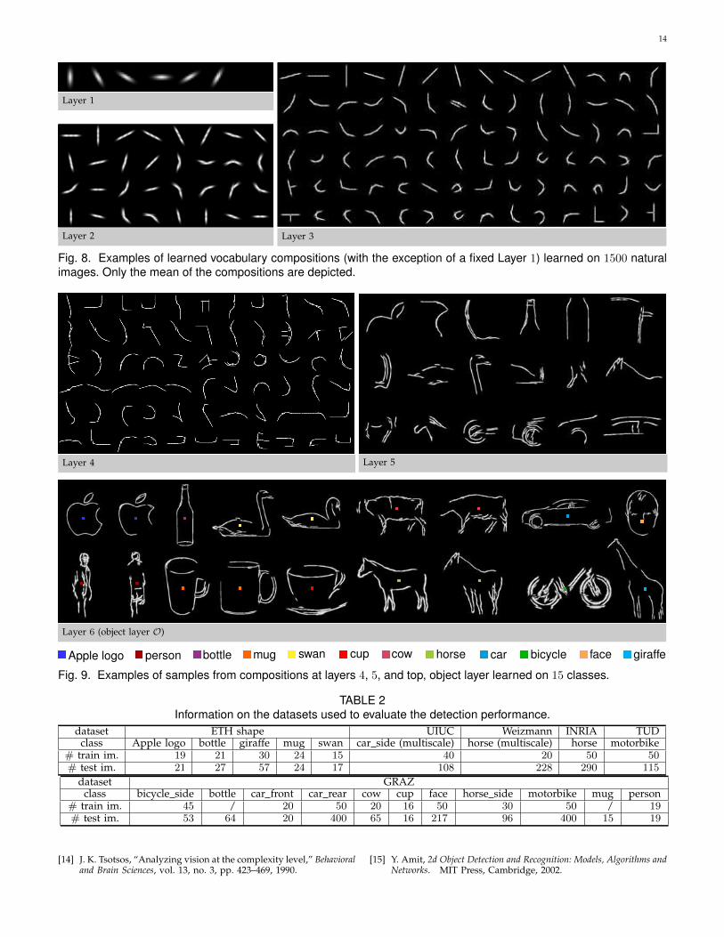
6.1 Natural statistics and object classificationWe applied our learning approach to a collection of1500 natural images. Learning was performed only upto layer 3, with the complete learning process takingroughly 5 hours. The learned hierarchy consisted of 160compositions on Layer 2 and 553 compositions on Layer3. A few examples from both layers are depicted in Fig. 8(note that the images shown are only the mean shapesmodeled by the compositions). The learned features in-clude corners, end-stopped lines, various curvatures, T-and L-junctions. Interestingly, these structures resemblethe ones predicted by the Gestalt rules [23].
To put the proposed hierarchical framework in re-lation to other categorization approaches which focusprimarily shape, the learned 3−layer vocabulary wastested on the Caltech-101 database [60]. The Caltech-101dataset contains images of 101 different object categorieswith the additional background category. The numberof images varies from 31 to 800 per category, with theaverage image size of roughly 300× 300 pixels.
Each image was processed at 3 scales spaced apartby√
2. The scores of the hidden states were combined

11
with a linear one-versus-all SVM classifier [61]. This wasdone as follows: for each image a vector of a dimensionequal to the number of compositions at the particu-lar layer was formed. Each dimension of the vector,which corresponds to a particular type of a composition(e.g. an L-junction) was obtained by summing over allscores of the hidden states coding this particular type ofcomposition. To increase the discriminative information,a radial sampling was used similarly as in [62]: eachimage was split into 5 orientation bins and 2 distancesfrom the image center, for which separate vectors (asdescribed previously) were formed and consequentlystacked together into one, high-dimensional vector.
The results, averaged over 8 random splits of trainand test images, are reported in Table 1 with classifica-tion rates of existing hierarchical approaches shown forcomparison. For 15 and 30 training images we obtained a60.5% and 66.5% accuracy, respectively, which is slightlybetter than the most related hierarchical approaches [12],[63], [32], comparable to those using more sophisticateddiscriminative methods [64], [65], and slightly worsethan those using additional information such as coloror regions [66].
We further tested the classification performance byvarying the number of training examples. For testing,50 examples were used for the classes where this waspossible and less otherwise. The classification rate wasnormalized accordingly. In all cases, the result was av-eraged over 8 random splits of the data. The results arepresented and compared with existing methods in Fig. 7.We only compare to approaches that use shape informa-tion alone and not also color and texture. Overall, betterperformance has been obtained in [67].
TABLE 1Average classification rate (in %) on Caltech 101.
Ntrain = 15 Ntrain = 30
Mutch et al. [63] 51 56Ommer et al. [12] / 61.3Ahmed at al. [65] 58.1 67.2Yu at al. [64] 59.2 67.4Lee at al. [34] 57.7 65.4Jarrett at al. [32] / 65.5our approach 60.5 66.5
6.2 Object class detection
The approach was tested on 15 diverse object classesfrom standard recognition datasets. The basic informa-tion is given in Table 2. These datasets are known tobe challenging because they contain a high amount ofclutter, multiple objects per image, large scale differencesof objects and exhibit a significant intra class variability.
For training we used the bounding box informationof objects or the masks if they were available. Eachobject was resized so that its diagonal in an image wasapproximately 250 pixels. For testing, we up-scaled eachtest image by a factor 3 and used 6 scales for objectdetection. When evaluating the detection performance, a
0 5 10 15 20 25 3010
20
30
40
50
60
70
Ntrain
Per
form
ance
(%
)
Caltech−101 Performance
ApproachesGriffin, Holub & Perona (2007)Zhang, Berg, Maire & Malik (2006)Lazebnik, Schmid & Ponce (2006)Wang, Zhang, Fei−Fei (2006)Grauman & Darrell (2005)Mutch and Lowe (2006) Our approach
Fig. 7. Classification performance on Caltech-101.
detection is counted as correct, if the predicted boundingbox bfg coincides with the ground truth bgt more than50%: area(bfg∩bgt)
area(bfg∪bgt) > 0.5. On the ETH dataset and INRIAhorses this threshold is lowered to 0.3 to enable a faircomparison with the related work [50]. The performanceis given either with recall at equal error rate (EER) orpositive detection rate at low FPPI, depending on thetype of results reported on these datasets thus-far.
6.2.1 Single class learning and performanceWe first evaluated our approach to learn and detecteach object class individually. We report the training andinference times, and the accuracy of detection, which willthen be compared to the multi-class case in Sec. 6.2.2 totest the scalability of the approach.
Training time. To train a class it takes on average 20−25minutes. For example, it takes 23 minutes to train onApple logo, 31 for giraffe, 17 for swan, 25 for cow, and 35for the horse class. For comparison, in Shotton et al. [4],training on 50 horses takes roughly 2 hours (on a 2.2GHz machine using a C# implementation).
Inference time. Detection for each individual class takesfrom 2− 4 seconds per image, depending on the size ofthe image and the amount of texture it contains. Otherrelated approaches report approx. 5 to 10 times highertimes (in seconds): [38]: 20− 30, [41]: 16.9, [68]: 20, [1]:12− 18, however, at slightly older hardware.
Detection performance. The ETH experiments are per-formed in a 5-fold cross-validation obtained by sampling5 subsets of half of the class images at random. The testset for evaluating detection consists of all the remain-ing images in the dataset. The detection performanceis given as the detection rate at the rate of 0.4 false-positives per image (FPPI), averaged over the 5 trials asin [50]. The detection performance is reported in Table 3.Similarly, the results for the INRIA horses are given in a5-fold cross-validation obtained by sampling 5 subsets of50 class images at random and using the remaining 120for testing. The test set also includes 170 negative imagesto allow for a higher FPPI rate. With respect to [50], weachieve a better performance for all classes, most notably

12
for giraffes (24.7%). Our method performs comparablyto a discriminative framework by Fritz and Schiele [68].Better performances have recently been obtained by Majiand Malik [69] (93.2%) and Ommer and Malik [70](88.8%) using Hough voting and SVM-based verification.To the best of our knowledge, no other hierarchicalapproach has been tested on this dataset so far.
For the experiments on the rest of the datasets wereport the recall at EER. The results are given in Table 3.Our approach achieves competitive detection rates withrespect to the state-of-the-art. Note also that [37], [6] used150 training examples of motorbikes, while we only used50 (to enable a fair comparison with [3] on GRAZ).
While the performance in a single-class case is compa-rable to the current state-of-the-art, the main advantageof our approach are its computational properties whenthe number of classes is higher, as demonstrated next.
6.2.2 Multi-class learning and performanceTo evaluate the scaling behavior of our approach wehave incrementally learned 15 classes one after another.
The learned vocabulary. A few examples of the learnedshapes at layers 4 to 6 are shown in Fig.9 (only samplesfrom the generative model are depicted). An exampleof a complete object-layer composition is depicted inFig. 13. It can be seen that the approach has learnedthe essential structure of the class well, not missing anyimportant shape information.
Degree of composition sharing among classes. To see howshared are the vocabulary compositions between classesof different degrees of similarity, we depict the learnedvocabularies for two visually similar classes (motor-bike and bicycle), two semi-similar classes (giraffe andhorse), and two dissimilar classes (swan and car front)in Fig. 10. The nodes correspond to compositions and thelinks denote the compositional relations between themand their parts. The green nodes represent the compo-sitions used by both classes, while the specific colorsdenote class specific compositions. If a spatial relationis shared as well, the edge is also colored green. Thecomputational advantage of our hierarchical representa-tion over flat ones [3], [6], [2] is that the compositionsare shared at several layers of the vocabulary, whichsignificantly reduces the overall complexity of inference.Even for the visually dissimilar classes, which may nothave any complex parts in common, our representationis highly shared at the lower layers of the hierarchy.
To evaluate the shareability of the learned composi-tions among the classes, we use the following measure:
deg share(`) =1
|Ω`|∑ω`∈Ω`
(# of classes that use ω`)− 1
# of all classes− 1,
defined for each layer ` separately. By “ω` used by classc” it is meant that the probability of ω` under c is notequal to zero. To give some intuition behind the measure:deg share = 0 if no composition from layer ` is shared(each class uses its own set of compositions), and it is 1
if each composition is used by all the classes. Fig. 12 (b)plots the values for the learned 15−class representation.Beside the mean (which defines deg share), the plotsalso show the standard deviation.
The size of the vocabulary. It is important to test howthe size of the vocabulary (the number of compositionsat each layer) scales with the number of classes, sincethis has a direct influence on inference time. We reportthe size as a function of the number of learned classesin Fig. 11. For the “worst case” we take the independenttraining approach: a vocabulary for each class is learnedindependently of other classes and we sum over thesizes of these separate vocabularies. One can observea logarithmic tendency especially at the lower layers.This is particularly important because the complexityof inference is much higher for these layers (becausethey contain less discriminative compositions which aredetected more numerously in images). Although the fifthlayer contains highly class specific compositions, one canstill observe a logarithmic increase in size. The final,object layer, is naturally linear in the number of classes,but it does, however, learn less object models than is thenumber of all training examples of objects in each class.
We further compare the scaling tendency of our ap-proach with the one reported for a non-hierarchical rep-resentation by Opelt et al. [3]. The comparison is givenin Fig. 12 (a) where the worst case is taken as in [3]. Wecompare the size of the class-specific vocabulary at layer5, where the learned compositions are of approximatelythe same granularity as the features used in [3]. We ad-ditionally compare the overall size of the vocabulary (asum of the sizes over all layers). Our approach achievesa substantially better scaling tendency, which is due tosharing at multiple layers of representation. This, on theone hand, compresses the overall representation, whileit also attains a higher variability of the compositions inthe higher layers and consequently, a lower number ofthem are needed to represent the classes.
Fig. 12 (d) shows the storage demands as a functionof the number of learned classes. This is the actual sizeof the vocabulary stored on a hard disk. Notice that the15-class hierarchy takes only 1.6Mb on disk.
Inference time. We further test how the complexity ofinference increases with each additional class learned.We randomly sample ten images per class and report thedetection times averaged over all selected images. Thetimes are reported as a function of the number of learnedclasses. The results are plotted in Fig. 12 (c), showing thatthe running times are significantly faster than the “worstcase” (the case of independent class representation, inwhich each separate class vocabulary is used to detectobjects). It is worth noting, that it takes only 16 secondsper image to apply a vocabulary of all 15 classes.
Detection performance. We additionally test the multi-class detection performance. The results are presented inTable 4 and compared with the performance of the singleclass vocabularies. The evaluation was the following. Forthe single class case, a separate vocabulary was trained
13
on each class and evaluated for detection independentlyof other classes. For the multi-class case, a joint multi-class vocabulary was learned (as explained in Sec. 6.2.2)and detection was performed as proposed in Sec. 5.2,that is, we allowed for competition among hypothesesexplaining partly the same regions in an image.
Overall, the detection rates are slightly worse in themulti-class case, although in some cases the multi-classcase outperformed the independent case. The main rea-son for a slightly reduced performance is due to the factthat the representation is generative and is not trained todiscriminate between the classes. Consequently, it doesnot separate similar classes sufficiently well and a wronghypothesis may end up inhibiting the correct one. Aspart of the future work, we plan to also incorporate morediscriminative information into the representation andincrease the recognition accuracy in the multi-class case.On the other hand, the increased performance for themulti-class case for some objects is due to feature sharingamong the classes, which results in better regularizationand generalization of the learned representation.
7 SUMMARY AND CONCLUSIONS
We proposed a novel approach which learns a hierarchi-cal compositional shape vocabulary to represent multi-ple object classes in an unsupervised manner. Learningis performed bottom-up, from small oriented contourfragments to whole-object class shapes. The vocabularyis learned recursively, where the compositions at eachlayer are combined via spatial relations to form largerand more complex shape compositions.
Experimental evaluation was two-fold: one that showsthe capability of the method to learn generic shapestructures from natural images and uses them for objectclassification, and another one that utilizes the approachin multi-class object detection. We have demonstrateda competitive classification and detection performance,fast inference even for a single class, and most impor-tantly, a logarithmic growth in the size of the vocabulary(at least in the lower layers) and, consequently, scalabil-ity of inference complexity as the number of modeledclasses grows. The observed scaling tendency of ourhierarchical framework goes well beyond that of a flatapproach [3]. This provides an important showcase thathighlights learned hierarchical compositional vocabular-ies as a suitable form of representing a higher numberof object classes.
8 FUTURE WORK
There are numerous directions for future work. One im-portant aspect would be to include multiple modalitiesin the representation. Since many object classes havedistinctive textures and color, adding this informationto our model would increase the range of classes thatthe method could be applied to. Additionally, modelingtexture could also boost the performance of our currentmodel: since textured regions in an image usually have
a lot of noisy feature detections, they are currently moresusceptible to false positive object detections. Having amodel of texture could be used to remove such regionsfrom the current inference algorithm. Another interestingpossible way of dealing with this issue would be to usehigh quality bottom-up region proposals to either re-score our detections or be used in our inference. Usingsegmentation in detection has recently been shown as avery promising approach [72], [73], [48].
Part of our ongoing work is to make the approach scal-able to a large number of object classes. To achieve this,several improvements and extensions are still needed.We will need to incorporate the discriminative informa-tion into the model (to distinguish better between similarclasses), make use of contextual information to improveperformance in the case of ambiguous information (smallobjects, large occlusion, etc) and use attention mecha-nisms to speed-up detection in large complex images.Furthermore, a taxonomic organization of object classescould further improve the speed of detection [46] and,possibly, also the recognition rates of the approach.
ACKNOWLEDGMENTS
This research has been supported in part by the follow-ing funds: Research program Computer Vision P2-0214(Slovenian Ministry of Higher Education, Science andTechnology) and EU FP7-215843 project POETICON.
REFERENCES[1] R. Fergus, P. Perona, and A. Zisserman, “Weakly supervised scale-
invariant learning of models for visual recognition,” InternationalJ. of Computer Vision, vol. 71, no. 3, pp. 273–303, March 2007.
[2] A. Torralba, K. P. Murphy, and W. T. Freeman, “Sharing visualfeatures for multiclass and multiview object detection,” IEEETrans. Patt. Anal. and Mach. Intell., vol. 29, no. 5, pp. 854–869, 2007.
[3] A. Opelt, A. Pinz, and A. Zisserman, “Learning an alphabet ofshape and appearance for multi-class object detection,” Interna-tional J. of Computer Vision, vol. 80, no. 1, pp. 16–44, 2008.
[4] J. Shotton, A. Blake, and R. Cipolla, “Multi-scale categorical objectrecognition using contour fragments,” IEEE Trans. Patt. Anal. andMach. Intell., vol. 30, no. 7, pp. 1270–1281, 2008.
[5] V. Ferrari, L. Fevrier, F. Jurie, and C. Schmid, “Groups of adjacentcontour segments for object detection,” IEEE Trans. Patt. Anal. andMach. Intell., vol. 30, no. 1, pp. 36–51, 2008.
[6] B. Leibe, A. Leonardis, and B. Schiele, “Robust object detectionwith interleaved categorization and segmentation,” InternationalJ. of Computer Vision, vol. 77, no. 1-3, pp. 259–289, 2008.
[7] G. Bouchard and B. Triggs, “Hierarchical part-based visual objectcategorization,” in CVPR, 2005, pp. 710–715.
[8] S. Ullman and B. Epshtein, Visual Classification by a Hierarchy of Ex-tended Features, ser. Towards Category-Level Object Recognition.Springer-Verlag, 2006.
[9] S. Fidler, M. Boben, and A. Leonardis, “Learning hierarchicalcompositional representations of object structure,” in Object Cat-egorization: Computer and Human Vision Perspectives, S. Dickinson,A. Leonardis, B. Schiele, and M. J. Tarr, Eds. CambridgeUniversity Press, 2009.
[10] S. Zhu and D. Mumford, “A stochastic grammar of images.”Foundations and Trends in Computer Graphics and Vision, vol. 2, no. 4,pp. 259–362, 2006.
[11] S. Fidler and A. Leonardis, “Towards scalable representations ofvisual categories: Learning a hierarchy of parts,” in CVPR, 2007.
[12] B. Ommer and J. M. Buhmann, “Learning the compositionalnature of visual objects,” in CVPR, 2007.
[13] R. Girshick, P. Felzenszwalb, and D. McAllester, “Object detectionwith grammar models,” in NIPS, 2009.
14
Layer 1
Layer 2 Layer 3
Fig. 8. Examples of learned vocabulary compositions (with the exception of a fixed Layer 1) learned on 1500 naturalimages. Only the mean of the compositions are depicted.
Layer 4 Layer 5
Layer 6 (object layer O)
Apple logo person bottle mug swan cup cow horse car bicycle face giraffe
Fig. 9. Examples of samples from compositions at layers 4, 5, and top, object layer learned on 15 classes.
TABLE 2Information on the datasets used to evaluate the detection performance.
dataset ETH shape UIUC Weizmann INRIA TUDclass Apple logo bottle giraffe mug swan car side (multiscale) horse (multiscale) horse motorbike
# train im. 19 21 30 24 15 40 20 50 50# test im. 21 27 57 24 17 108 228 290 115
dataset GRAZclass bicycle side bottle car front car rear cow cup face horse side motorbike mug person
# train im. 45 / 20 50 20 16 50 30 50 / 19# test im. 53 64 20 400 65 16 217 96 400 15 19
[14] J. K. Tsotsos, “Analyzing vision at the complexity level,” Behavioraland Brain Sciences, vol. 13, no. 3, pp. 423–469, 1990.
[15] Y. Amit, 2d Object Detection and Recognition: Models, Algorithms andNetworks. MIT Press, Cambridge, 2002.
15
TABLE 3Detection results. On the ETH shape and INRIA horses we report the detection-rate (in %) at 0.4 FPPI averaged overfive random splits train/test data. For all the other datasets the results are reported as recall at equal-error-rate (EER).
ETHshape
class [50] [68] our approachapplelogo 83.2 (1.7) 89.9 (4.5) 87.3 (2.6)bottle 83.2 (7.5) 76.8 (6.1) 86.2 (2.8)giraffe 58.6 (14.6) 90.5 (5.4) 83.3 (4.3)mug 83.6 (8.6) 82.7 (5.1) 84.6 (2.3)swan 75.4 (13.4) 84.0( 8.4) 78.2 (5.4)average 76.8 84.8 83.7
INRIA horse 84.8(2.6) / 85.1(2.2)
class related work our approachUIUC car side, multiscale 90.6 [63] 93.5 [66] 93.5Weizmann horse multiscale 89.0 [4] 93.0 [71] 94.3TUD motorbike 87 [6] 88 [37] 83.2
class [3] [4] our approachface 96.4 97.2 94
GRAZ
bicycle side 72 67.9 68.5bottle 91 90.6 89.1cow 100 98.5 96.9cup 81.2 85 85car front 90 70.6 76.5car rear 97.7 98.2 97.5horse side 91.8 93.7 93.7motorbike 95.6 99.7 93.0mug 93.3 90 90person 52.6 52.4 60.4
(a) (b) (c)
Fig. 10. Sharing of compositions between classes. Each plot shows a vocabulary learned for two object classes. The bottomnodes in each plot represent the 6 edge orientations, one row up denotes the learned second layer compositions, etc. The sixthrow (from bottom to top) are the whole-shape, object-layer compositions (i.e., different aspects of objects in the classes), whilethe top layer is the class layer which pools the corresponding object compositions together. The green nodes denote the sharedcompositions, while specific colors show class-specific compositions. From left to right: Vocabularies for: (a) two visually similarclasses (motorbike and bicycle), (b) two semi-similar object classes (giraffe and horse), (c) two visually dissimilar classes (swanand car front). Notice that even for dissimilar object classes, the compositions from the lower layers are shared between them.
1 2 3 4 5 6 7 8 9 10 11 12 13 14 150
50
100
150
number of classes
num
ber
of c
ompo
sitio
ns
Size of representation (# classes)
worst case (linear)our approach
Layer 2
1 2 3 4 5 6 7 8 9 10 11 12 13 14 150
50
100
150
200
number of classes
num
ber
of c
ompo
sitio
ns
Size of representation (# classes)
worst case (linear)our approach
Layer 3
1 2 3 4 5 6 7 8 9 10 11 12 13 14 150
50
100
150
200
250
300
350
number of classes
num
ber
of c
ompo
sitio
ns
Size of representation (# classes)
worst case (linear)our approach
Layer 4
1 2 3 4 5 6 7 8 9 10 11 12 13 14 150
100
200
300
400
number of classes
num
ber
of c
ompo
sitio
nsSize of representation (# classes)
worst case (linear)our approach
Layer 5
Fig. 11. Size of representation (the number of compositions per layer) as a function of the number of learned classes. “Worstcase” denotes the sum over the sizes of single-class vocabularies.
1 2 3 4 5 6 7 8 9 10 11 12 13 14 150
200
400
600
800
1000
1200
1400
number of classes
num
ber
of v
ocab
ular
y fe
atur
es
Size of representation, flat vs hier.
worst case (linear)Opelt et al. 2008layer 5whole hierarchy
1 2 3 4 5
00.10.20.30.40.50.60.70.80.9
1
Degree of sharing
layer
degr
ee o
f sha
ring
15 classesmotorbike−bikegiraffe−horseswan−car front
2 4 6 8 10 12 140
10
20
30
40
50
60
70
number of classes
infe
renc
e tim
e pe
r im
age
(sec
)
Inference time per image (# classes)
worst case (linear)our approach
1 2 3 4 5 6 7 8 9 10 11 12 13 14 150
500
1000
1500
2000
2500
3000
number of classes
cum
ulat
ive
size
on
disk
(K
b)
Storage (size on disk)
worst case (linear)our approach
(a) (b) (c) (d)
Fig. 12. From left to right: (a) A comparison in scaling to multiple classes of the approach by Opelt et al. [3] (flat) and ourhierarchical approach; (b) Degree of sharing for the multi-class vocabulary; (c) Average inference time per image as a function ofthe number of learned classes; (d) Storage (size of the hierarchy stored on disk) as a function of the number of learned classes.
16
TABLE 4Comparison in detection accuracy for single- and multi-class object representations and detection procedures.
class Apple bottle giraffe mug swan horse cow mbike bicycle car front car side car rear face person cupmeasure detection rate (in %) at 0.4 FPPI recall (in %) at EER
single 88.6 85.5 83.5 84.9 75.8 84.5 96.9 83.2 68.5 76.5 97.5 93.5 94.0 60.4 85.0multi 84.1 80.0 80.2 80.3 72.7 82.3 95.4 83.2 64.8 82.4 93.8 92.0 93.0 62.5 85.0
(a) (b) (c)
Fig. 13. One learned object-layer composition ωO for (a) bottle, (b) giraffe, and (c) bicycle, with the complete model structureshown. The blue patches denote the limiting circular regions, the color regions inside them depict the spatial relations (Gaussians).The nodes are the compositions in the vocabulary. Note that each composition models the distribution over the compositions fromthe previous layer for the appearance of its parts. For clarity, only the most likely composition for the part is decomposed further.
Fig. 14. Examples of detections. The links show the most probable hidden state activation for a particular (top-layer) classdetection. The links are color-coded to denote different classes.
[16] S. Fidler, M. Boben, and A. Leonardis, “Evaluating multi-classlearning strategies in a generative hierarchical framework forobject detection,” in NIPS, 2009.
[17] M. Leordeanu, R. Sukhtankar, and M. Hebert, “Object and cat-egory recognition from pairwise relations between features,” inCVPR, 2007.
[18] A. Shokoufandeh, L. Bretzner, D. Macrini, M. Demirci, C. Jonsson,and S. Dickinson, “The representation and matching of categoricalshape,” Computer Vision and Image Understanding, vol. 103, pp.139–154, 2006.
[19] S. Sarkar and K. Boyer, Computing Perceptual Organization inComputer Vision. Singapore: World Scientific, 1994.
[20] S. Geman, D. Potter, and Z. Chi, “Composition systems,” Quarterlyof Applied Mathematics, vol. 60, no. 4, pp. 707–736, 2002.
[21] J. Schwartz and P. Felzenszwalb, “Hierarchical matching of de-
formable shapes,” in CVPR, 2007.[22] S. Edelman, N. Intrator, and J. S. Jacobson, “Unsupervised learn-
ing of visual structure,” in Biologically Motivated Computer Vision,2002, pp. 629–642.
[23] M. Wertheimer, “Untersuchungen zur lehre von der gestalt.”Psychologische Forschung: Zeitschrift fuer Psychologie und ihre Gren-zwissenschaften, vol. 4, no. 1, pp. 301–350, 1923.
[24] G. J. Ettinger, “Hierarchical object recognition using libraries ofparameterized model sub-parts,” MIT, Tech. Rep., 1987.
[25] S. Dickinson, “The evolution of object categorization and the chal-lenge of image abstraction,” in Object Categorization: Computer andHuman Vision Perspectives, S. Dickinson, A. Leonardis, B. Schiele,and M. J. Tarr, Eds. Cambridge University Press, 2009.
[26] J. Utans, “Learning in compositional hierarchies: Inducing thestructure of objects from data,” in NIPS, 1994, pp. 285–292.
17
[27] K. Fukushima, S. Miyake, and T. Ito, “Neocognitron: a neuralnetwork model for a mechanism of visual pattern recognition,”IEEE Systems, Man and Cyber., vol. 13, no. 3, pp. 826–834, 1983.
[28] M. Riesenhuber and T. Poggio, “Hierarchical models of objectrecognition in cortex,” Nature Neuroscience, vol. 2, no. 11, pp. 1019–1025, 1999.
[29] T. Serre, L. Wolf, S. Bileschi, M. Riesenhuber, and T. Poggio,“Object recognition with cortex-like mechanisms,” IEEE Trans.Patt. Anal. and Mach. Intell., vol. 29, no. 3, pp. 411–426, 2007.
[30] T. Masquelier and S. J. Thorpe, “Unsupervised learning of visualfeatures through spike timing dependent plasticity,” PLoS Com-putational Biology, vol. 3, no. 2, pp. 832–838, 2007.
[31] M. A. Ranzato, F. J. Huang, Y. L. Boureau, and Y. LeCun, “Un-supervised learning of invariant feature hierarchies with applica-tions to object recognition,” in CVPR, 2007.
[32] K. Jarrett, K. Kavukcuoglu, M. A. Ranzato, and Y. LeCun, “What isthe best multi-stage architecture for object recognition?” in ICCV,2009.
[33] G. E. Hinton, “Learning multiple layers of representation,” Trendsin Cognitive Sciences, vol. 11, no. 10, pp. 428–434, 2007.
[34] H. Lee, R. Grosse, R. Ranganath, and A. Y. Ng, “Convolutionaldeep belief networks for scalable unsupervised learning of hier-archical representations,” in ICML, 2009, pp. 609–616.
[35] E. Sudderth, A. Torralba, W. T. Freeman, and A. Willsky, “De-scribing visual scenes using transformed objects and parts,” In-ternational J. of Computer Vision, vol. 77, no. 1-3, pp. 291–330, 2008.
[36] B. Epshtein and S. Ullman, “Semantic hierarchies for recognizingobjects and parts,” in CVPR, 2007.
[37] K. Mikolajczyk, B. Leibe, and B. Schiele, “Multiple object classdetection with a generative model,” in CVPR, 2006, pp. 26–36.
[38] S. Todorovic and N. Ahuja, “Unsupervised category modeling,recognition, and segmentation in images,” IEEE Trans. Patt. Anal.and Mach. Intell., vol. 30, no. 12, 2008.
[39] F. Scalzo and J. H. Piater, “Statistical learning of visual featurehierarchies,” in Workshop on Learning, CVPR, 2005.
[40] F. Fleuret and D. Geman, “Coarse-to-fine face detection,” Interna-tional J. of Computer Vision, vol. 41, no. 1/2, pp. 85–107, 2001.
[41] L. Zhu, C. Lin, H. Huang, Y. Chen, and A. Yuille, “Unsupervisedstructure learning: Hierarchical recursive composition, suspiciouscoincidence and competitive exclusion,” in ECCV, vol. 2, 2008,pp. 759–773.
[42] Y. Amit, D. Geman, and X. Fan, “A coarse-to-fine strategy formulticlass shape detection,” IEEE Trans. Patt. Anal. and Mach.Intell., vol. 26, no. 12, pp. 1606–1621, 2004.
[43] Y. Amit and D. Geman, “A computational model for visualselection,” Neural Computation, vol. 11, no. 7, pp. 1691–1715, 1999.
[44] M. Marszałek and C. Schmid, “Constructing category hierarchiesfor visual recognition,” in ECCV, ser. LNCS, vol. IV. Springer,2008, pp. 479–491.
[45] P. Zehnder, E. K. Meier, and L. V. Gool, “An efficient shared multi-class detection cascade,” in BMVC, 2008.
[46] S. Fidler, M. Boben, and A. Leonardis, “A coarse-to-fine taxonomyof constellations for fast multi-class object detection.” in ECCV,2010, pp. 687–700.
[47] A. Krizhevsky, I. Sutskever, and G. E. Hinton, “Imagenet classifi-cation with deep convolutional neural networks.” in NIPS, 2012,pp. 1106–1114.
[48] R. Girshick, J. Donahue, T. Darrell, and J. Malik, “Rich featurehierarchies for accurate object detection and semantic segmenta-tion,” in CVPR, 2014.
[49] R. C. Nelson and A. Selinger, “Large-scale tests of a keyed,appearance-based 3-d object recognition system,” Vision Research,vol. 38, no. 15-16, pp. 2469–2488, 1998.
[50] V. Ferrari, L. Fevrier, F. Jurie, and C. Schmid, “Accurate objectdetection with deformable shape models learnt from images,” inCVPR, 2007.
[51] R. Fergus, P. Perona, and A. Zisserman, “A sparse object categorymodel for efficient learning and exhaustive recognition,” in CVPR,vol. 1, 2005, pp. 380–397.
[52] S. Fidler, M. Boben, and A. Leonardis, “Optimization frameworkfor learning a hierarchical shape vocabulary for object classdetection.” in BMVC, 2009.
[53] S. Fidler, G. Berginc, and A. Leonardis, “Hierarchical statisticallearning of generic parts of object structure,” in CVPR, 2006, pp.182–189.
[54] S. Fidler, M. Boben, and A. Leonardis, “Similarity-based cross-layered hierarchical representation for object categorization,” inCVPR, 2008.
[55] P. Felzenszwalb, R. Girshick, D. McAllester, and D. Ramanan,“Object detection with discriminatively trained part based mod-els.” IEEE Trans. Patt. Anal. and Mach. Intell., vol. 32, no. 9, 2010.
[56] N. Petkov, “Biologically motivated computationally intensive ap-proaches to image pattern recognition,” Future Generation Com-puter Systems, vol. 11, no. 4-5, pp. 451–465, 1995.
[57] M. Weber, M. Welling, and P. Perona, “Towards automatic discov-ery of object categories,” in CVPR, 2000, pp. 2101–2108.
[58] S. Belongie, J. Malik, and J. Puzicha, “Shape matching and objectrecognition using shape contexts,” IEEE Transactions on PatternAnalysis and Machine Intelligence, vol. 24, pp. 509–522, 2001.
[59] S. Fine, Y. Singer, and N. Tishby, “The hierarchical hidden markovmodel: Analysis and applications,” Machine Learning, vol. 32,no. 1, pp. 41–62, 1998.
[60] L. Fei-Fei, R. Fergus, and P. Perona, “Learning generative visualmodels from few training examples: an incremental bayesian ap-proach tested on 101 object categories.” in IEEE CVPR, Workshopon Generative-Model Based Vision, 2004.
[61] T. Joachims, “Making large-scale support vector machine learningpractical,” pp. 169–184, 1999.
[62] H. Zhang, A. C. Berg, M. Maire, and J. Malik, “Svm-knn: Dis-criminative nearest neighbor classification for visual categoryrecognition,” in CVPR, vol. 2, 2006, pp. 2126–2136.
[63] J. Mutch and D. G. Lowe, “Multiclass object recognition withsparse, localized features,” in CVPR, 2006, pp. 11–18.
[64] K. Yu, W. Xu, and Y. Gong, “Deep learning with kernel regular-ization for visual recognition,” in NIPS, 2008, pp. 1889–1896.
[65] A. Ahmed, K. Yu, W. Xu, Y. Gong, and E. P. Xing, “Traininghierarchical feed-forward visual recognition models using transferlearning from pseudo tasks,” in ECCV, vol. III, 2009, pp. 69–82.
[66] N. Ahuja and S. Todorovic, “Connected segmentation tree – ajoint representation of region layout and hierarchy,” CVPR, 2008.
[67] M. Varma and D. Ray, “Learning the discriminative power-invariance trade-off,” in ICCV, 2007.
[68] M. Fritz and B. Schiele, “Decomposition, discovery and detectionof visual categories using topic models,” in CVPR, 2008.
[69] S. Maji and J. Malik, “Object detection using a max-margin houghtransform,” in CVPR, 2009.
[70] B. Ommer and J. Malik, “Multi-scale object detection by clusteringlines,” in ICCV, 2009.
[71] J. Shotton, A. Blake, and R. Cipolla, “Efficiently combining con-tour and texture cues for object recognition,” in BMVC, 2008.
[72] J. R. R. Uijlings, K. E. A. van de Sande, T. Gevers, and A. W. M.Smeulders, “Selective search for object recognition.” InternationalJ. of Computer Vision, vol. 104, no. 2, 2013.
[73] S. Fidler, R. Mottaghi, A. Yuille, and R. Urtasun, “Bottom-upsegmentation for top-down detection,” in CVPR, 2013.