Embed Size (px)
Citation preview

Learning a Test Oracle towards Automating
Image Segmentation Evaluation
By
Kambiz Frounchi
A thesis submitted to the Faculty of Graduate Studies and Research
in partial fulfillment of the requirements for the degree of
Master of Applied Science
Ottawa-Carleton Institute of Electrical and Computer Engineering
Department of Systems and Computer Engineering
Carleton University
Ottawa, Ontario, Canada
December 2008
1

1*1 Library and Archives Canada
Published Heritage Branch
395 Wellington Street Ottawa ON K1A0N4 Canada
Bibliotheque et Archives Canada
Direction du Patrimoine de I'edition
395, rue Wellington Ottawa ON K1A0N4 Canada
Your file Votre reference ISBN: 978-0-494-47512-6 Our file Notre reference ISBN: 978-0-494-47512-6
NOTICE: The author has granted a nonexclusive license allowing Library and Archives Canada to reproduce, publish, archive, preserve, conserve, communicate to the public by telecommunication or on the Internet, loan, distribute and sell theses worldwide, for commercial or noncommercial purposes, in microform, paper, electronic and/or any other formats.
AVIS: L'auteur a accorde une licence non exclusive permettant a la Bibliotheque et Archives Canada de reproduire, publier, archiver, sauvegarder, conserver, transmettre au public par telecommunication ou par Plntemet, prefer, distribuer et vendre des theses partout dans le monde, a des fins commerciales ou autres, sur support microforme, papier, electronique et/ou autres formats.
The author retains copyright ownership and moral rights in this thesis. Neither the thesis nor substantial extracts from it may be printed or otherwise reproduced without the author's permission.
L'auteur conserve la propriete du droit d'auteur et des droits moraux qui protege cette these. Ni la these ni des extraits substantiels de celle-ci ne doivent etre imprimes ou autrement reproduits sans son autorisation.
In compliance with the Canadian Privacy Act some supporting forms may have been removed from this thesis.
Conformement a la loi canadienne sur la protection de la vie privee, quelques formulaires secondaires ont ete enleves de cette these.
While these forms may be included in the document page count, their removal does not represent any loss of content from the thesis.
Canada
Bien que ces formulaires aient inclus dans la pagination, il n'y aura aucun contenu manquant.
The undersigned hereby recommend to
The Faculty of Graduate Studies and Research
acceptance of the thesis
Learning a Test Oracle towards Automating
Image Segmentation Evaluation Submitted by
Kambiz Frounchi
In partial fulfillment of the requirements for the degree of
Master of Applied Science
Professor L. C. Briand (Co-Supervisor)
Professor Y. Labiche (Co-Supervisor)
Professor V. Aitken (Department Chair)
Carleton University
December 2008
2
ABSTRACT
Image segmentation is the act of extracting particular structures of interest from an
image. A lot of time and effort is spent in order to evaluate image segmentation
algorithms. If the image segmentation algorithm does not provide accurate enough results
or in verification and validation terms fails, the technical expert needs to modify it and re
run the whole test suite to verify the revised image segmentation algorithm. This process
is repeated as the image segmentation algorithm evolves to its final acceptable version
where the test suite passes. This evaluation process is mostly done manually at the
moment and is therefore very time consuming, requiring the presence of reliable experts.
In this thesis, a solution is proposed that uses machine learning techniques to semi-
automate this evaluation process. During the initial learning phase, the expert is required
to evaluate segmentations manually. The similarity between the segmentations produced
by the initial versions of the segmentation algorithm is found by applying a set of
comparison measures to pairs of segmentations from the same subject. This information
is used by different machine learning algorithms to devise a classifier that can classify a
pair of segmentations as being diagnostically consistent or inconsistent. In a second
phase, once a valid classifier is learnt, a segmentation produced by any new version of
the image segmentation algorithm under test will be automatically deemed correct or
incorrect depending on whether it is diagnostically consistent with the segmentations
previously deemed correct. In this second phase, there is no need for any intervention
from human experts. To demonstrate the performance of the approach, we have applied
the solution to the evaluation of the left heart ventricle segmentation and have gotten very
promising results. This solution also helps find the best performing machine learning
techniques and the similarity measures with the most discriminating power in the context
of the application.
3

ACKNOWLEDGEMENTS
I would like to thank Professors Briand and Labiche for their active support throughout
this research work. This thesis was a joint collaboration between Carleton University and
the software and medical imaging departments in Siemens Corporate Research. I would
like to thank Leo Grady and Rajesh Subramanyan in Siemens Corporate Research for
their help throughout my work. Last but not least I would like to thank my family and
friends for their moral support.
4
TABLE OF CONTENTS
ABSTRACT 3
ACKNOWLEDGEMENTS 4
TABLE OF CONTENTS 5
LIST OF FIGURES 7
LIST OF TABLES 8
1 INTRODUCTION 9
2 RELATED WORK 13
3 BACKGROUND 18
3.1 Image segmentation comparison techniques 18 3.1.1 Overlap measures 20 3.1.2 Geometrical measures 25 3.1.3 Volume difference measures 36
3.2 Machine learning techniques 36
4 IMAGE SEGMENTATION EVALUATION ORACLE DESIGN 41
4.1 Segmentation evaluations swimlane 42
4.2 Learning classifier swimlane 44
4.3 Tool support architecture 46
5 CASE STUDY: LEFT HEART VENTRICLE SEGMENTATION EVALUATION 50
5.1 Examples 52
5.2 Experiment setup 55
5.3 Description of classifiers 57 5.3.1 J48 57 5.3.2 PART 63 5.3.3 JRIP 63
5.4 Attribute correlations 64
5.5 Attribute sets 66
5.6 Classifiers 68 5.6.1 J48 68 5.6.2 PART 76 5.6.3 JRIP 78 5.6.4 Conclusion 81
5.7 Classifier Performance Comparison 83 5.7.1 Effect of using different measure types 85 5.7.2 Effect of using different data mining techniques 86 5.7.3 Effect of using different attribute selection techniques 87 5.7.4 Conclusion 89
5.8 Tools 89
5.9 Timing considerations 90
5.10 Conclusions 94
5

6 CONCLUSIONS AND FUTURE WORK 95
7 REFERENCES 98
6
LIST OF FIGURES
Figure 1.1 - Manual Image Segmentation Evaluation Process 10
Figure 3.1 - Four mutually exclusive overlapping regions between the Segmentation Under Test (SUT) and the True Segmentation (TS) 24
Figure 3.2 - A grid point 26
Figure 3.3 - Left: Segmentation; Center: dA distance transform; Right: d% distance transform
[15] 28
Figure 3.4 - Hausdorff s distance between sets A and B [15] 30
Figure 3.5 -PFOM rates B and C to be equally similar to A [23] 31
Figure 3.6 - Object is geometrically symmetrical around the principal axes (x'i, x'2, x 3) 35
Figure 4.1 - Semi-automated image segmentation algorithm evaluation process 41
Figure 4.2 - Structural components of the automated oracle 47
Figure 5.1 - Correct Left Heart Ventricle Segmentation 53
Figure 5.2 - Incorrect Segmentation (oversegmentation to the left atrium) 53
Figure 5.3 - Incorrect Segmentation (Segmenting an incorrect region i.e. the right ventricle).... 54
Figure 5.4 - Incorrect Segmentation (severe undersegmentation) 54
Figure 5.5 - A sample decision tree 58
Figure 5.6 - Split of instances by attributes 1 and 2 60
Figure 5.7 - (a) Top: J48 classifier trained with simple measures (OV) (b) Bottom: J48 classifier trained with the simple measures selected using J48 wrapper (OVW) 71
Figure 5.8 - (a) Top: J48 classifier trained with geometrical measures (G) (b) Bottom: J48 classifier trained with the geometrical measures selected using J48 wrapper (GW) 73
Figure 5.9 - (a) Top: J48 classifier trained with all comparison measures (A) (b) Bottom: J48 classifier trained with the comparison measures selected using J48 wrapper (AW) 75
Figure 5.10 - Accuracy of J48, PART and JRIP classifiers versus each attribute set 83
Figure 5.11 - Kappa Statistic of J48, PART and JRIP classifiers versus each attribute set 84
Figure 5.12 - Area under ROC curve of J48, PART and JRIP classifiers versus each attribute set 84
Figure 5.13 - Time consumption of comparison measures (x-axis = segmentation pair number, y-axis = time consumption in seconds) 93
7

LIST OF TABLES
Table 3.1 - Two-class prediction outcomes 39
Table 4.1 - Mapping between classifier results and the evaluation of the unknown image segmentation 43
Table 4.2 - Consistency of two segmentations 45
Table 4.3 - Table of all outputs produced by the previous versions of the SUT (version < Vi) and their corresponding evaluations 48
Table 4.4 - An example showing how the Consistency to Correctness Mapper module obtains the correctness of the OUT 49
Table 5.1 -Details of case study 55
Table 5.2 - Attributes used for machine learning 56
Table 5.3 - Spearman's rank correlation coefficient between highly correlated attribute pairs... 65
Table 5.4 - Attribute sets and their selection criteria 66
Table 5.5 - J48 configuration parameters 68
Table 5.6 - Configuration parameters for JRIP 79
Table 5.7 - Comparison of classifier accuracies with respect to the attribute set category used for training (simple, geometrical, all) 86
Table 5.8 - Comparison of classifier accuracies with respect to the data mining technique (J48, PART, JRIP) 87
Table 5.9 - Comparison of classifier accuracies with respect to the use of filters and wrappers on the simple measures for training 88
Table 5.10 - Comparison of classifier accuracies with respect to the use of filters and wrappers on the geometrical measures for training 88
Table 5.11- Comparison of classifier accuracies with respect to the use of filters and wrappers on all of the measures for training 88
Table 5.12-Average comparison measure calculation times 94
8
1 INTRODUCTION
Image segmentation is the act of extracting content from an image. Specifically, image
segmentation refers to the act of delineating a particular object or structure of interest
from an image [11]. Image segmentation algorithms have been devised to automatically
segment an image without the need of an expert manually delineating the object of
interest from the image. Experience has shown that devising an image segmentation
algorithm is an iterative approach, as illustrated in Figure 1.1. The technical expert who
devises each successive version of the image segmentation algorithm has to revise the
initially devised image segmentation algorithm many times (steps 2, 3 and 4), verifying
each revision manually (step 3) until the verification results indicate an acceptable
revision of the image segmentation algorithm. To test each revision of the image
segmentation algorithm, a sample set of subjects (or images) is used, a segmentation of
each subject is obtained by applying the revision of the segmentation algorithm that is
under test to each subject, and a few technical and medical experts verify the correctness
of the produced image segmentations by grading them (step 3): Typically, a 1 to 5 scale
is used. In software testing terms, the experts play the role of the (test) oracle that decides
whether a test case (i.e., a subject in this case) passes or not (i.e., the subject segmentation
is adequate). If all of the image segmentations receive a satisfactory grade by all of the
experts, then the image segmentation algorithm is considered to be satisfactory. Other
criteria may be considered such as enforcing that specific segmented subjects, that have
particular diagnostically significant features, get a minimum acceptable grade for the
image segmentation algorithm to be considered valid. Otherwise, the image segmentation
algorithm has to be revised (step 4) and the same manual testing procedure has to be
repeated for the newly revised image segmentation algorithm (steps 2 and 3).
This testing procedure is time-consuming and expensive as it requires the availability of
medical experts to verify the segmentations. It may suffer from human errors made by the
medical expert during the manual verification of a large number of images, and is also
prone to different opinions by different medical experts (inter-expert variability) [12].
Providing semi-automated support for this manual verification and validation process will
9
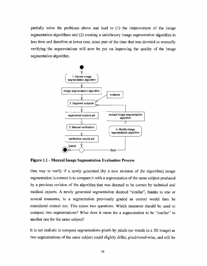
partially solve the problems above and lead to (1) the improvement of the image
segmentation algorithms and (2) creating a satisfactory image segmentation algorithm in
less time and therefore at lower cost, since part of the time that was devoted to manually
verifying the segmentations will now be put on improving the quality of the image
segmentation algorithm.
1 1: Devise image
segmentation algorithm
_ ! image segmentation algorithm
JL 2: Segment subjects
subjects
< -
X segmented subject set
±
revised image segmentation algorithm
IT 3: Manual verification
X 4: Modify image
segmentation algorithm
verification results set
[pass]
[fail]
Figure 1.1 - Manual Image Segmentation Evaluation Process
One way to verify if a newly generated (by a new revision of the algorithm) image
segmentation is correct is to compare it with a segmentation of the same subject produced
by a previous revision of the algorithm that was deemed to be correct by technical and
medical experts. A newly generated segmentation deemed "similar", thanks to one or
several measures, to a segmentation previously graded as correct would then be
considered correct too. This raises two questions: Which measures should be used to
compare two segmentations? What does it mean for a segmentation to be "similar" to
another one for the same subject?
It is not realistic to compare segmentations pixels by pixels (or voxels in a 3D image) as
two segmentations of the same subject could slightly differ, pixel/voxel-wise, and still be
10

equivalent from the point of view of the expert. Instead, there exist a number of
measures, currently used and empirically validated in the image processing domain that
can be used to compare segmentations.
One way to use such similarity measures to compare segmentations is to set a threshold
and argue that if a new segmentation diverges from a segmentation previously
characterized as correct by more than the threshold value, then the new segmentation is
not correct. However, we would need to define a threshold beforehand, which could only
be highly subjective and unlikely to be optimal. Instead, we intend to rely on a machine
learning algorithm to develop decision models (classifiers). This decision model would
characterize which similarity measures and which deviations of similarity measure values
between new segmentations and previous segmentations (deemed to be correct) are
indicative of (in)correct segmentations. In this way while one measure may not be a good
indicator of the similarity between a pair of segmentations, but many such measures, each
good at reflecting some aspect of the similarity between the two segmentations, can be
combined by the machine learning algorithm to indicate the consistency of the
segmentation pair with high accuracy.
As a result, once we have learnt a sufficiently accurate decision mode (classifier), testing
the image segmentations (step 3 in Figure 1.1) will no longer require human intervention.
In other words, human expert knowledge will only be required to learn the decision
model, which will then be used to support automated decisions. Therefore, the whole
image segmentation algorithm testing process will be semi-automated. This will mean
fewer opportunities for medical expert errors, no inter-expert variability, less time spent
by the experts to verify the different revisions of the image segmentation algorithm, and
as mentioned before more time for improving the quality of the image segmentation
algorithm.
In a nutshell the main contributions of this thesis are (1) devising a re-usable semi-
automated approach that attempts to solve the oracle problem for testing (medical) image
segmentation algorithms. In doing so, the approach (2) helps to find the appropriate
n

machine learning techniques and (3) similarity measures pertinent to the application.
Last, the approach is applied on the problem of left heart ventricle segmentations.
The remainder of this thesis is structured as follows. It starts with a discussion of related
work on the oracle problem (Chapter 2). Chapter 3 gives some background on image
segmentation comparison techniques and machine learning methods. Chapter 4 explains
our generic approach towards the semi-automated evaluation of image segmentation
algorithms. The results obtained in the case study (left heart ventricle segmentation
algorithm verification) are explained in Chapter 5. Chapter 6 concludes the thesis with a
discussion of future steps.
12

2 RELATED WORK
There is a large body of work in the image processing field on studying and improving
image segmentation algorithms. This body of work is however out of the scope of this
thesis and is therefore not further discussed here.
An oracle is a procedure that assesses whether the observed behavior of the software
under test matches its expected behavior. The oracle will output either a "yes" or "no"
and it may include an explanation as to why this decision was made [4]. Whether we can
define such a procedure to assess the correctness of the software under test is referred to
as the oracle problem.
Defining an oracle is not a trivial task and it may not be feasible to define one at all times.
Even if it is theoretically possible to define an oracle, it may not be practically possible to
verify the correctness of the software under test in a reasonable amount of time while
putting a reasonable amount of effort [2]. In [1], software that we cannot devise an oracle
for are referred to as un-testable software and lie into three categories:
1) Software where the output is unknown. An example for this situation is given
in [3]; consider a program that analyzes petri-nets and outputs the probability
of being in a particular state; It is very difficult to verify whether all the digits
of the output probability are correct or not.
2) Software where the output is of a very large volume and thus cannot be
verified in a reasonable amount of time.
3) Software where the tester has a misconception about its correct behavior. This
is usually the case where the oracle is based on a different specification than
the specification that the implementation of the software under test is based
on.
13
Different solutions have been proposed to the oracle problem. One approach is design
redundancy [1,[2], where different implementations of the same specification are
produced. If the outputs produced by two different implementations on the same input
differ, we can conclude that there is a problem: either one of the two versions has a
problem, or the two versions both have a problem. When the outputs are the same, we
may express some confidence that the software under test is behaving correctly, but this
may still not be a valid assumption as both programs may be producing similar incorrect
results. However, if the two versions were independently designed, this should be
unlikely. The assumption of independence in multi-version programming has been
explored in [8]. The results of this empirical study show that the independence
assumption in multi-version programming may not hold at all times and care should be
taken on the reliability of multi-version programming. More than two independently
designed versions can also be used: a consensus strategy has to be adopted where if the
outputs from a large number of the implementations agree with the output of the software
under test, the software is deemed to have produced the correct output. Implementing
multiple versions of the same specification of the software under test is a time-consuming
and expensive activity. The effort going into implementing the extra versions may be as
much as implementing the software under test and the agreement of the outputs of the
software under test and the other version(s) does not necessarily imply that the output of
the software under test is correct. It is proposed in [1] that high level languages should be
used for the implementation of the extra versions, but this may not be a feasible choice at
all times. For example, using high level languages for the implementation of highly
memory-intensive and cpu-intensive applications would result in a very high time
overhead for obtaining the results of these slow programs and thus immensely increase
the time required for testing the software under test. However, some researchers have
argued that multi-version programming does not necessarily add a significant amount to
the cost since the implementation of the software is just a minor part of the overall
software development process [10]. The notion of multi versions of a program is also
used in regression testing [3]. In this context, previous versions of the program can be
used as references of correct behavior as the software evolves.
14

Another approach to the oracle problem is data redundancy. In this approach, the output
of the software under test is verified by testing how it behaves with respect to other
inputs. For example, consider an algorithm to calculate the sin(x) for some input x. Using
71 71 the identitysin(a + 6) = sin(a)sin( 6) + sin( a)sin(6), if (a+b = x), sin(x) can be
verified by changing the value of a and b [3]. This approach works very well when such
mathematical identities can be found in the particular application. Other examples of the
use of this technique is when we know that the output of the software under test for a
given input data should vary slightly if we feed it with data that is very close to the input
data. Large variations would indicate to the oracle that the software under test is not
behaving properly. N-copy programming [6] is also a data redundancy technique.
Although introduced in the context of fault tolerance the principle can be used in testing.
In N-copy programming, a re-expression algorithm is used to re-express the input data in
N different forms (i.e. make N copies of the data) which are all logically equivalent to the
input data. The outputs of executing the program on the N different copies are fed into a
voter which can be thought of as the oracle in a testing scenario. If a majority of the N
outputs are very different from the output produced by the input data we can conclude
that the software under test is behaving incorrectly. In the case where the majority agrees,
we gain more confidence that the software is acting correctly. Using data redundancy,
there is no overhead of implementing extra versions of the software under test which
makes the data redundancy method cheaper than design redundancy, but the challenge is
to find appropriate input/output relationships.
Another alternative to design and data redundancy is consistency checks. In this approach
the oracle checks if the outputs of the software under test are consistent, i.e., whether they
conform to some known facts. For example in a program that outputs probabilities, one
consistency check is checking that the output probability cannot exceed one or be
negative. An alternative is to narrow down the output domain to a plausible output
domain and check whether the consistency check is valid or not for those outputs when
executing the test cases [1]. This kind of checking cannot prove that the software under
test is correct but it can help find faults in the software.
15
Another alternative towards tackling the oracle problem is to only test the software under
test on simplified data, i.e., the data that the output is known for [2]. The obvious
drawback to this approach is that the software under test usually has faulty behavior in
the more complicated scenarios.
In the case where formal specifications exist for the software under test, researchers have
proposed methods to derive oracles from the formal specifications. This has been
investigated for real-time systems in [7], where the test class consists of some test
executions or sequences of stimuli. Test oracles in the form of assertions are obtained
using symbolic interpretation of the specifications for each control point. A discussion on
oracles that are composed of assertions based on properties specified either in first order
logic or computation tree logic is given in [5]. Assertions under the form of pre and post
conditions can also be used as test oracles [9].
In [19], machine learning is used to evaluate which of the two segmentations produced by
different segmentation algorithms or with different parameterizations of the same
segmentation algorithm is better in delineating the objects of interest. In their study they
combine the evaluations made by standalone methods to make this decision. Standalone
methods evaluate the goodness of a segmentation by applying some quantitative measure
to the segmentation. The quantities measured may be for example the color uniformity of
the labeled region, which requires information from the original image in addition to just
the labeling from the segmentation. Decision trees are used to model these standalone
methods though how the decision trees are constructed and how accurately they model
the standalone methods is not described accurately. The evaluations made by each of the
decision trees are combined using meta-learning, which essentially combines the
decisions of the different decision trees, each predicting which of the two segmentations
are better, and makes a final decision. A fundamental difference in the use of machine
learning in their research work and ours is that we try to use machine learning to find the
best subset of comparison measures between two segmentations that could predict the
consistency of two segmentations while in [19] they use standalone methods which are
applied to only one segmentation each time. Also, the similarity measures that we define
do not require any information from the original images (such as information regarding
16

color, texture, etc.), only using information from the segmentations (the extent and shape
of labeling) to get a measure of consistency, while the standalone methods in [19]
generally do.
3 BACKGROUND
In this Chapter some background information will be given on two subjects of interest in
this research work:
1. Image segmentation comparison techniques: As mentioned in the Introduction, we
propose to study the similarities between segmentations with a number of
measures. A discussion of some popular similarity measures that are used for
comparing two segmentations is given in Section 3.1.
2. Machine learning techniques: As mentioned in the Introduction, we intend to rely
on a machine learning algorithm to identify what it means for two segmentations
to be similar. Different machine learning techniques will be evaluated to find an
appropriate one in our context. A very brief discussion of the available machine
learning techniques and the methods that are used to evaluate them is given in
Section 3.2.
3.1 Image segmentation comparison techniques
Image segmentation is the act of extracting content from an image. Specifically, image
segmentation refers to the act of delineating a particular object or structure of interest
from an image [11]. Image segmentation algorithms have been devised to automatically
segment an image without the need of an expert manually delineating the object of
interest from the image. These image segmentation algorithms have to be verified and
validated. This can be done by evaluating the correctness of the segmented images. Some
methods that are used to evaluate the correctness of the segmented images, in the medical
domain are:
• Manual evaluation: The segmentation is compared with the manual segmentation
produced by a medical expert, or directly evaluated by the medical expert.
• Physical and Computational Phantoms: Phantoms are either physical or
computational models that are obtained from a known true segmentation for
18
evaluating image segmentation algorithms [12]. The segmentation obtained from
applying the segmentation algorithm to a physical or computational phantom is
compared with the known true segmentation that the physical or computational
phantom is constructed for.
Manual evaluation suffers from the following obstacles [12]:
• The time, effort, and cost entailed when relying on medical experts who are
scarce resources.
• Medical expert error: The medical expert may wrongly segment the image due to
poor vision or factors related to the quality and resolution of the image.
• Inter-expert variability: Different experts may segment the image differently,
causing confusion in finding the surrogate of truth.
Phantoms also have disadvantages. Physical phantoms usually do not depict a realistic
anatomical model and digital phantoms use a very simplistic model of the image
acquisition process [16].
In summary, in order to evaluate the correctness of an image segmentation algorithm,
generated segmentations have to be compared with some surrogate of truth. This
surrogate may be the manual delineation of the segmentation obtained from a medical
expert, the true segmentation that the phantom is constructed for, or a different
segmentation algorithm (version) that was assessed to be correct by a human expert. This
last form is more relevant to the context of this research work since the segmentation
algorithm development process is iterative: during iteration /', i.e., when building version i
of the segmentation algorithm, segmentations produced during the evaluation of iteration
j Q<i), i.e., when building version/ of the segmentation algorithm, that were assessed as
correct can be used to check version /. When comparing segmentations produced by
versions / and j of the segmentation algorithm, three families of measures can be
considered: measures that simply look at the extent of overlapping of the two
segmentations (Section 3.1.1), measures that compare the shapes of the two
19
segmentations, referred here to as geometrical measures (Section 3.1.2), and measures
that compare the volumes delineated by the two segmentations (Section 3.1.3).
A 2D digital picture is a grid of a finite number of pixels. Each pixel is denoted with its
location and a value at that location [15]. In the case of 3D digital images, the term voxel
is used instead of pixel, but in this text pixel refers interchangeably to both 2D and 3D
cases. The value associated with each pixel location could be the color of that location or
any other relevant value. In this text, the segmentation is considered as a digital picture
and the value associated with each pixel is its label in the segmentation.
3.1.1 Overlap measures
A label is an identifier of a particular structure of interest in an image. As a result of
segmenting an image, each point is associated with one to many labels. If each point is
associated with only one label, the segmentation is referred to as a hard segmentation.
Otherwise the segmentation is said to be fuzzy. Different overlapping measures can be
devised for these two kinds of segmentations.
3.1.1.1 Measures for hard segmentations
To compare hard segmentations, a number of similarity measures have been defined. The
main ones calculate the amount of overlap of the labeled regions between two
segmentations (usually the segmentation under test and the segmentation that is
considered to be the surrogate of truth):
• Dice Similarity Coefficient (DSC) [14]:
Equation 3.1 DSC - 2 N < L R - ^ N(LR„,) + N(LR„)
where LRsut is the labeled region in the Segmentation Under Test (SUT), LRts is
the labeled region in the True Segmentation (TS), and N(LR) is the number of
pixels in the labeled region LR.
20

• Tanimoto Coefficient (TC) [2]:
EqUa,i„„3.2 rc^m"".) N(LR„,uLR„)
The DSC and the TC coefficients have the same numerator which is the number of pixels
that overlap among the common labeled region of the segmentation under test and the
true segmentation. This number is divided by the total number of pixels in the two
labeled regions in DSC, and by the number of pixels in the union of the two labeled
regions in TC. Both of these measures are simply trying to measure the percentage of
common label between the segmentation under test and the true segmentation.
In the above two coefficients, each pixel in a segmentation is either in a labeled region or
is not, and no two labeled regions overlap in any one (hard) segmentation. In the simplest
case we only have two labels in a segmentation, one representing the regions where the
structure of interest is located and one representing the rest of the segmentation. The
notation in Equation 3.1 and Equation 3.2 assume there is only one region of interest
(which will be the case in our case studies). The notation can easily be extended to
account for more than two labels (e.g., by subscripting LR with the label name).
3.1.1.2 Measures for fuzzy segmentations
In fuzzy segmentations, each pixel may be a part of more than one label. The percentage
of involvement of each pixel/? in each labeled region / in S (the set of all the pixels in the
segmentation) can be represented by the membership
functionms/(/?)e [0,1], ms(/?) = ^Timsl(p) = l. Fuzzy segmentations are a better leLabels
representation of reality as different labels may overlap in medical images due to partial-
volume effects. Partial volume effects are caused when multiple tissues contribute to the
same pixel causing the blurring of the medical image in those set of pixels [4].
Fuzzy segmentations can be compared using fuzzy measures. Before defining the fuzzy
measures in more detail, we first provide some fuzzy set theory definitions: Equation 3.3
to Equation 3.7. In these definitions, A and B are two sets of pixels.
21
The membership functions for each pixelp in the intersection (AnB), union {AVJB)
and difference (A - B) of the sets A and B are defined in Equation 3.3, Equation 3.4, and
Equation 3.6.
Equation 3.3 mAnB (p) = £ a, (MIN(mAl (p), mBl (p))) leLabels
Equation3.4 mAwB(p) = J ] a, ^MAXim^ip^m^ip)) leLabels pePixels
v .. , - , . \mAj(p)-mBJ(p) mAl(p)-mBl(p)>0 Equation 3.5 "^ . / ( /OH. " ,
0 otherwise
Equation 3.6 mA_B{p)= ^ a, ^mA_BJ(p) leLabels pePixels
The cardinality for set A is defined in Equation 3.7.
Equation 3.7 \A\= J ] a, J ] ^ ^ ) ) leLabels pePixels
In Equation 3.3 and Equation 3.4, MIN(mAl(p),mBl(p)) is the minimum of the assigned
membership of label / to pixel p in the sets A and B, MAX(mA l (p), mB, (p)) is the
maximum of the assigned membership of label / to pixel p in the sets A and B. In
Equation 3.3 to Equation 3.7, a, e [0,1], "^a, = 1, where al is the weight of each label. leLabels
Assigning different weights to different labels is useful when some labels are of more
importance than others.
A fuzzy overlap definition for comparing two segmentations (TCMF) is defined1 in
Equation 3.8, where SUT and TS refer to the set of pixels that are respectively in the
segmentation under test and the true segmentation.
This definition is similar to equation (3) in [14], but described in a different way.
22
/ , mSUTnTS \P)
Equation 3.8 TC^ = ^ — / , mSUTuTS \P)
psPixels
Equation 3.8 is a good overlap comparison measure when the image segmentation
algorithm produces a multi-label fuzzy segmentation, but fuzzy segmentations are a
generalization of hard segmentations as are fuzzy measures a generalization of non-fuzzy
measures, so Equation 3.8 can be used for hard segmentations too. In TCMF, a value of
zero would indicate zero overlap between the segmentation under test and the true
segmentation while a value of 1 indicates 100 percent overlap between them.
3.1.1.3 Statistical decision theory measures
Some measures derived from statistical decision theory have been suggested for
comparing segmentations [12]. The measures are based on the definition of four mutually
exclusive regions in Figure 3.1 for a 2-D situation, referred to as TP (True Positive), TN
(True Negative), FP (False Positive) and FN (False Negative). In the definition of TN, U
is the union of the four mutually exclusive regions: U = 7P u TN u FP u FN.
TP is the Truly Positive area, i.e., the intersection of the segmentation under test and the
true segmentation: TP = SUT n TS. TN is the Truly Negative area, i.e., the area that
does not intersect with neither the true segmentation nor the segmentation under test:
TN -U- SUT -TS. FP is the Falsely Positive area, i.e., the area in the segmentation
under test that does not intersect with the true segmentation: FP = SUT - TS. FN is the
Falsely Negative area, i.e., the area in the true segmentation that does not intersect with
the segmentation under test: FN = TS- SUT.
23
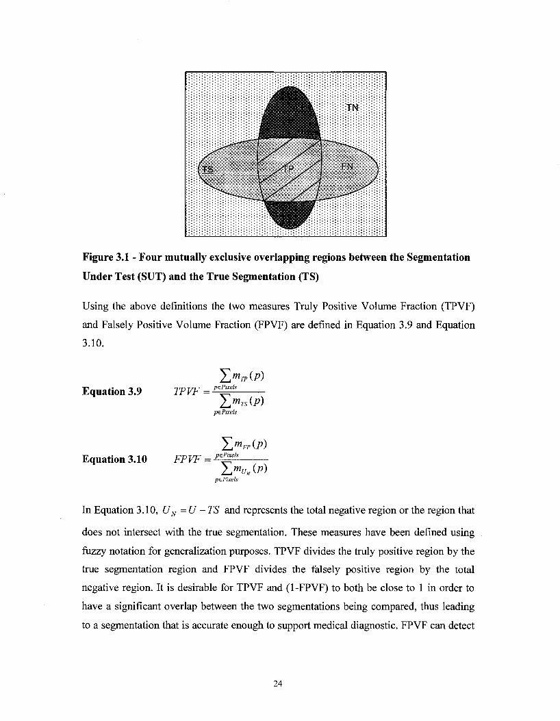
Figure 3.1 - Four mutually exclusive overlapping regions between the Segmentation
Under Test (SUT) and the True Segmentation (TS)
Using the above definitions the two measures Truly Positive Volume Fraction (TPVF)
and Falsely Positive Volume Fraction (FPVF) are defined in Equation 3.9 and Equation
3.10.
Equation 3.9 TPVF = pePixd$
YamTs(P) pePixels
Equation 3.10 Yimpp(p)
FPVF pE. Pixels
p&Pixels
In Equation 3.10, UN=U -TS and represents the total negative region or the region that
does not intersect with the true segmentation. These measures have been defined using
fuzzy notation for generalization purposes. TPVF divides the truly positive region by the
true segmentation region and FPVF divides the falsely positive region by the total
negative region. It is desirable for TPVF and (1-FPVF) to both be close to 1 in order to
have a significant overlap between the two segmentations being compared, thus leading
to a segmentation that is accurate enough to support medical diagnostic. FPVF can detect
24
the situations where the segmentation under test has a high percentage of overlap with the
correct segmentation but incorrectly labels other regions too.
3.1.2 Geometrical measures
The measures defined in Section 3.1.1 are all overlap measures calculating the amount of
overlap between the two segmentations under comparison. Geometrical measures go
beyond calculating the overlap. They take into account the differences in the shapes of
the two segmentations under comparison, capturing differences such as the size and
position of the segmentation boundaries. Overlap measures may be sufficient in many
cases to detect severe oversegmentation (segmentation under test labeling pixels that are
not of interest) or severe undersegmentation (segmentation under test not labeling pixels
that are of interest) but they do not perform well in situations where the segmentation
under test has a reasonably high percentage of overlap with the correct segmentation, but
incorrectly labels some pixels of interest that make the segmentation diagnostically
unacceptable from the standpoint of a medical expert and thus the segmentation has to be
evaluated as incorrect. In these cases, geometrical measures may help capture the subtle
differences between the segmentation under test and the correct segmentation. We
present below the geometrical measures that are used in this research work.
3.1.2.1 Average Distance to Boundary Difference
Let S be any arbitrary set of pixels, d :SxS h-> R is a metric or distance function if it
satisfies the following condition [15]:
Equation 3.11 0 = d(p,p) < d(p,q) + d(q,p) = 2d(p,q) for allp,qeS
[S,dJ defines a metric space. A widely used metric is the Euclidean metric.
Using an n-dimensional Cartesian coordinates system, let p=(x\, x%..., x„) and q=(yi,
yz—, yn) be any two pixels in Rn (n>l). The Euclidean metric de is defined as follows
[15]:
Equation3.12 de(p,q) = ^(x, -yx)2 +••• + (*„ -yn)2
25

Some other widely used metrics are the city-block or Manhattan metric (Equation 3.13)
and the chessboard metric (Equation 3.14) [15].
Equation 3.13
Equation 3.14
dA(p,q) = \xx-x2 \ + \yx-y2
dg (P> <l) = m a x ^ - x2 \, \yx - y21}
If/? and q are restricted to Z (Z is the set of integers), d4(p,q) is the number of horizontal
or vertical unit-length steps (where only one coordinate changes) from/? to q. dg(p,q) can
also take diagonal moves where both coordinates change similar to the moves of a king in
chess (notice the resemblance between the names of these metrics and their definition).
To better visualize the city-block and chessboard metrics we can see from Figure 3.2 that
d4(p,q) = 3, d4(p,r) = 6 while d8(p,q) = 2, d8(p,r) = 4.
Ay
c>-
o -
Q—Q-=«—cp
<b €> 0 CD-—0 X
Figure 3.2 - A grid point
The reason for the <̂ and ds notation used in the city-block and chessboard metric
definitions is that each pixel has respectively 4 or 8 adjacent pixels (neighbors) where the
neighbors of the pixel/? are defined in Equation 3.15:
Equation 3.15 Na(p) = {qeZ2:da(p,q)<\}
where Na (/?) is the set of neighbor pixels of pixel/?, a is the number of neighbor pixels.
We can extend the chessboard metric to 3D (Equation 3.16) in which case each pixel has
26 neighbors.
26

Equation 3.16 c/26(/?,^) = max{|x1 -a^l-Vi "J^I 'K ~ZI\)
If S represents the image, <S> the segmentation, i.e. the set of labeled pixels in the
image, and < S > the set of non-labeled pixels in the image, for any metric d the d
distance transform of S associates with each pixel p of <S> the distance to < S >. This
distance is the minimum distance of pixel p to the boundary of < S > and to find it we
can scan the adjacent neighbor pixels to p, finding the closest one to the boundary and
assigning p the distance of the closest neighbor to the boundary plus the distance between
pixel p and that neighbor pixel.
In order to bring more intuition on how the distance map is calculated, we describe a two
pass algorithm to calculate the da (a e {4,8}) distance transform in the 2D context [15]
though a similar approach can be used in the 3D case:
1) Pass 1: scan S from left-to-right, top-to-bottom and calculate f(p) as follows:
f 0 ifpe<S> Equation 3.17 fl(p) = \
[min{/, (q) +1: q e B(p)} if p e < S >
B(p) for pixel p with coordinates (x,y), is the two pixels (x,y+l) and (x-l,y) if the
dA distance transform is used. In case of using the ds distance transform the neighbor
pixels with coordinates (x-l,y+l) and (x+l,y+l) are also considered.
2) Pass 2: scan S from right-to-left, bottom-to-top and calculate f2 (p) as follows.
Equation 3.18 ^ (P) = m i n ( / i (/>), / 2 (?) +1 : ? e A(p)}
A(p) for pixel p with coordinates (x,y), is the two pixels (x,y-l) and (x+l,y) if the
dA distance transform is used. In case of using the ds distance transform the neighbor
pixels with coordinates (x+l,y-l) and (x-l,y-l) are also considered.
The distance to the boundary of the segmentation for each pixel p in the segmentation S
can be calculated in Equation 3.19:
27
Equation 3.19 da (p, <S >) = f2 (p) for all p in S
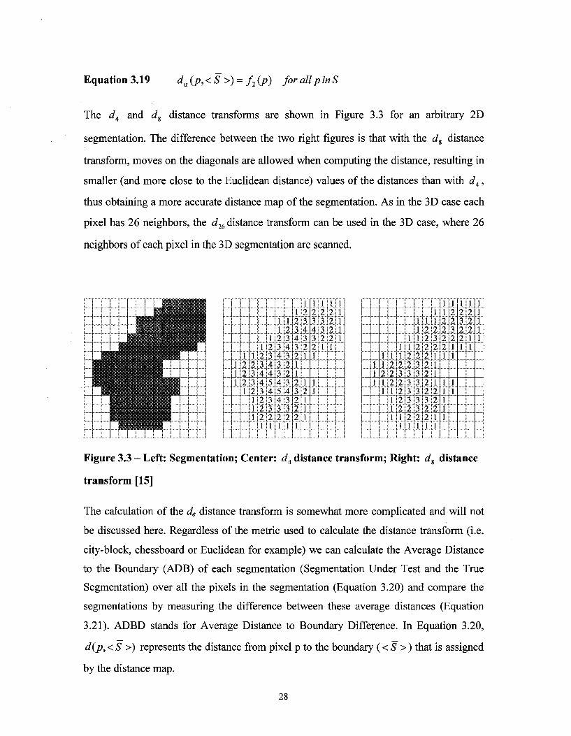
The d4 and ds distance transforms are shown in Figure 3.3 for an arbitrary 2D
segmentation. The difference between the two right figures is that with the ds distance
transform, moves on the diagonals are allowed when computing the distance, resulting in
smaller (and more close to the Euclidean distance) values of the distances than with dA,
thus obtaining a more accurate distance map of the segmentation. As in the 3D case each
pixel has 26 neighbors, the d16 distance transform can be used in the 3D case, where 26
neighbors of each pixel in the 3D segmentation are scanned.
1 1 1
\ ~~j
4-_ll, j 111 212 2 |3 213 112
11 U
1
1 2 3 4 4 3 2 2 2
i
l 2 3 4 4 5 4 3 3 2
i
l l 2 3 4 3 3 4 5 4 3 2
i
l 2 3 4 3 2 2 3 4 3 3 2
i
l 2 3 4 3 2 1 1 2 3 2 2 2
i
i 2
•f-3 2 1
1 2 1 I I.
1 2 3 4 3 2 1
1 1
1 2 3 3 2 1
1 2 2 2 2 1
1 1 1 1 1
—
1 1 1
1 1 2 1 1
1 2 2 2 1 1 1 I
1 1 2 3 2 2 2 2 1
i
l l 2 2 3 3 2 j 3 2 2
i
l i i 2 2 3 3 3 3 3 3 2 ........
1 2 2 2 2 2 2 2 2 3 2 2
i
l i 2 3 2 I 1 1 1 2 2 2 1
i
l l 2 2 2 2 1
1 1 1. 1 1
2
2 1 1
1 JL
1 2 3 2 2 1
1 2 2 2 1 1
1 1 1 1 1
Figure 3.3 - Left: Segmentation; Center: d4 distance transform; Right: d% distance
transform [15]
The calculation of the de distance transform is somewhat more complicated and will not
be discussed here. Regardless of the metric used to calculate the distance transform (i.e.
city-block, chessboard or Euclidean for example) we can calculate the Average Distance
to the Boundary (ADB) of each segmentation (Segmentation Under Test and the True
Segmentation) over all the pixels in the segmentation (Equation 3.20) and compare the
segmentations by measuring the difference between these average distances (Equation
3.21). ADBD stands for Average Distance to Boundary Difference. In Equation 3.20,
d(p, < S >) represents the distance from pixel p to the boundary (< S >) that is assigned
by the distance map.
28
2>(^<s>) Equation 3.20 ADB = ^ ^
number of pixels in< S >
Equation 3.21 ADBD = \ADBts - ADBsut \
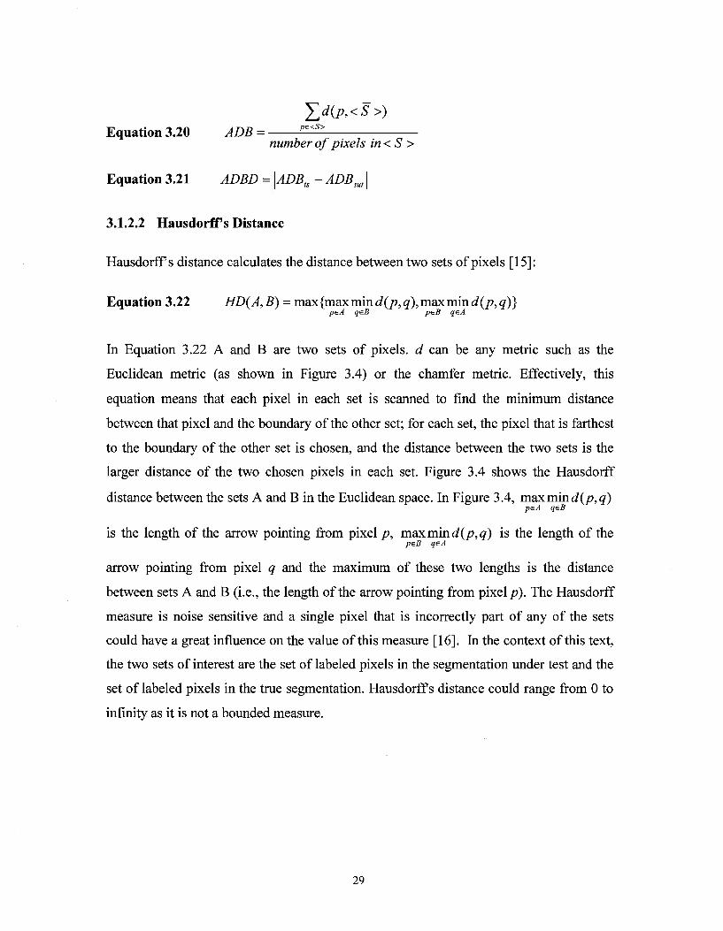
5A.22 Hausdorff s Distance
Hausdorff s distance calculates the distance between two sets of pixels [15]:
Equation 3.22 HD(A,B) = max{maxmind(p,q),maxmmd(p,q)} peA qeB psB q^A
In Equation 3.22 A and B are two sets of pixels, d can be any metric such as the
Euclidean metric (as shown in Figure 3.4) or the chamfer metric. Effectively, this
equation means that each pixel in each set is scanned to find the minimum distance
between that pixel and the boundary of the other set; for each set, the pixel that is farthest
to the boundary of the other set is chosen, and the distance between the two sets is the
larger distance of the two chosen pixels in each set. Figure 3.4 shows the Hausdorff
distance between the sets A and B in the Euclidean space. In Figure 3.4, maxmin<i(/>,g) peA qeB
is the length of the arrow pointing from pixel p, maxmmd(p,q) is the length of the psB qeA
arrow pointing from pixel q and the maximum of these two lengths is the distance
between sets A and B (i.e., the length of the arrow pointing from pixel p). The Hausdorff
measure is noise sensitive and a single pixel that is incorrectly part of any of the sets
could have a great influence on the value of this measure [16]. In the context of this text,
the two sets of interest are the set of labeled pixels in the segmentation under test and the
set of labeled pixels in the true segmentation. Hausdorff s distance could range from 0 to
infinity as it is not a bounded measure.
29
o set A
Gl^O KJ O KJ 0 O O O OX) O O O O O o o O X D O O O O O O O O^S D D D D D D • \ ^ / V ^ \—f \ ^ / X™^ htrnd® \rnid h*#*<4 WxJ! LHWXJ UremJ WKWI L™«J
O O O O O Q D & t L D D • • D
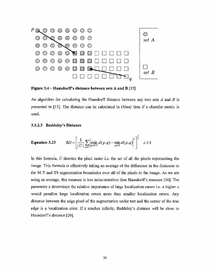
Figure 3.4 - Hausdorffs distance between sets A and B [15]
An algorithm for calculating the Hausdorff distance between any two sets A and B is
presented in [15]. The distance can be calculated in 0(mn) time if a chamfer metric is
used.
• set B
3.1.2.3 Baddeley's Distance
Equation 3.23 BD = U\ peU
™nd(p,q)-rnmd(p,q) qeSUT qzTS
z>\
In this formula, U denotes the pixel raster i.e. the set of all the pixels representing the
image. This formula is effectively taking an average of the difference in the distances to
the SUT and TS segmentation boundaries over all of the pixels in the image. As we are
using an average, this measure is less noise-sensitive than Hausdorffs measure [16]. The
parameter z determines the relative importance of large localization errors i.e. a higher z
would penalize large localization errors more than smaller localization errors. Any
distance between the edge pixel of the segmentation under test and the center of the true
edge is a localization error. If z reaches infinity, Baddeley's distance will be close to
Hausdorffs distance [20].
30
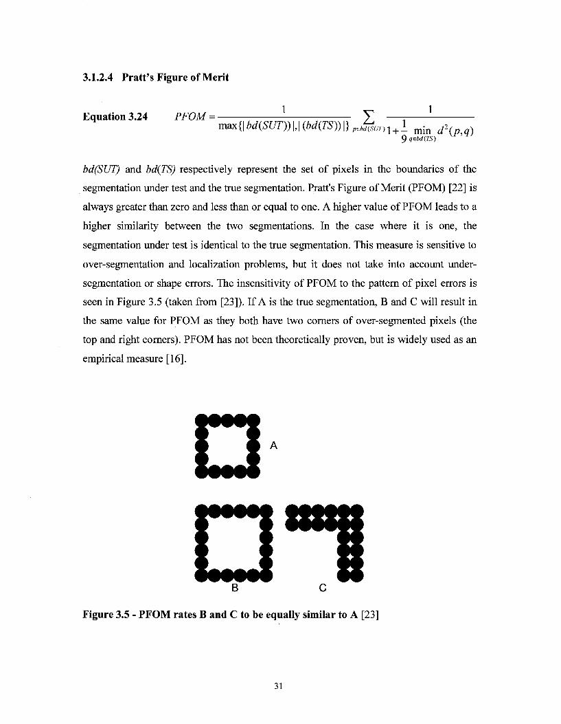
3.1.2.4 Pratt's Figure of Merit
Equation 3.24 PFOM = max{\bd(SUT))\,\(bd(TS))\}pebj?SUT)l + }_ m i n j . .
9qcbd(TS) KF,H'
bd(SUT) and bd(TS) respectively represent the set of pixels in the boundaries of the
segmentation under test and the true segmentation. Pratt's Figure of Merit (PFOM) [22] is
always greater than zero and less than or equal to one. A higher value of PFOM leads to a
higher similarity between the two segmentations. In the case where it is one, the
segmentation under test is identical to the true segmentation. This measure is sensitive to
over-segmentation and localization problems, but it does not take into account under-
segmentation or shape errors. The insensitivity of PFOM to the pattern of pixel errors is
seen in Figure 3.5 (taken from [23]). If A is the true segmentation, B and C will result in
the same value for PFOM as they both have two corners of over-segmented pixels (the
top and right corners). PFOM has not been theoretically proven, but is widely used as an
empirical measure [16].
O B
Figure 3.5 - PFOM rates B and C to be equally similar to A [23]
31
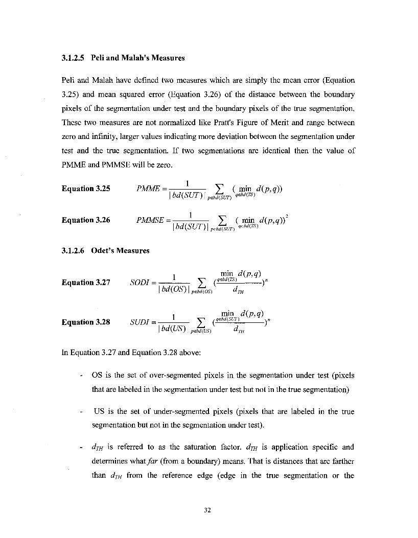
3.1.2.5 Peli and Malah's Measures
Peli and Malah have defined two measures which are simply the mean error (Equation
3.25) and mean squared error (Equation 3.26) of the distance between the boundary
pixels of the segmentation under test and the boundary pixels of the true segmentation.
These two measures are not normalized like Pratt's Figure of Merit and range between
zero and infinity, larger values indicating more deviation between the segmentation under
test and the true segmentation. If two segmentations are identical then the value of
PMME and PMMSE will be zero.
Equation3.25 PMME- Y ( min dip,a)) \bd{Sm)\p^SUT)\^rs) VFH"
Equation3.26 PMMSE = Y ( min d(p,q)f
3.1.2.6 Odet's Measures
1 min d(p,q) Equation 3.27 SODI = £ (̂ ™> )"
I bd(ub) I pebd(os) dTH
, min d(p, q) Equation 3.28 SUDI = £ (qehd(SUT) )"
| bd(Ub ) I pebd(us) dm
In Equation 3.27 and Equation 3.28 above:
- OS is the set of over-segmented pixels in the segmentation under test (pixels
that are labeled in the segmentation under test but not in the true segmentation)
US is the set of under-segmented pixels (pixels that are labeled in the true
segmentation but not in the segmentation under test).
- dm is referred to as the saturation factor, dm is application specific and
determines what^ar (from a boundary) means. That is distances that are farther
than dm from the reference edge (edge in the true segmentation or the
32
segmentation under test) are all considered to be the distance dm from the
reference edge. Dividing by dm normalizes the measures.
n is a scale factor that allows the assignment of different weights per pixel
depending on the pixel's distance to the boundary of the true segmentation i.e.
the pixels that are close to the boundary are weighted differently from the ones
that have a distance to the true segmentation boundary close to dm [16]. Setting
the scale factor n to a value more than 1 will result in considering the pixels
close to the reference edge as correct and only putting emphasis on the pixels
that have a distance close to the saturation factor dm while setting it to a value
that is more than zero and less than 1 will result in putting more emphasis on the
pixels that are close to the reference edge. Setting dm to smaller values leads to
evaluation with a higher accuracy (as we are over-emphasizing minor
discrepancies) but at the same time we may not be interested in minor
discrepancies between the two segmentations [21].
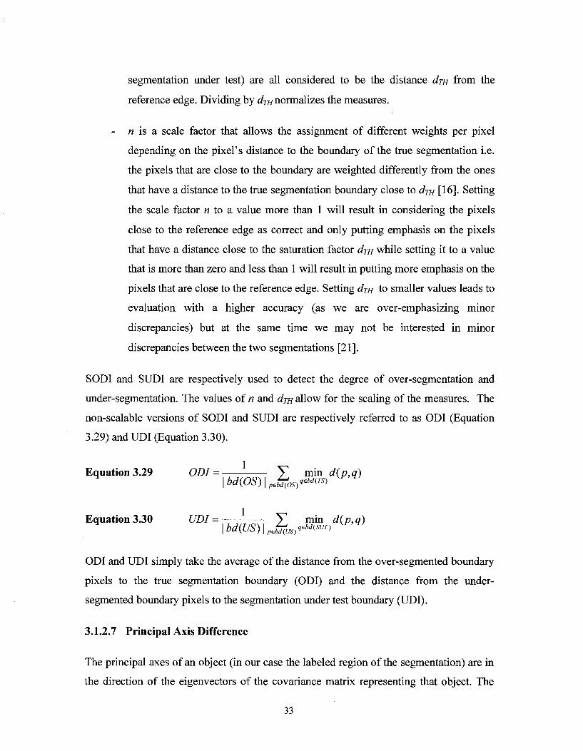
SODI and SUDI are respectively used to detect the degree of over-segmentation and
under-segmentation. The values of n and dm allow for the scaling of the measures. The
non-scalable versions of SODI and SUDI are respectively referred to as ODI (Equation
3.29) and UDI (Equation 3.30).
Equation 3.29 ODI = Y min dip,a)
Equation 3.30 UDI = Y min d(p,q)
ODI and UDI simply take the average of the distance from the over-segmented boundary
pixels to the true segmentation boundary (ODI) and the distance from the under-
segmented boundary pixels to the segmentation under test boundary (UDI).
3.1.2.7 Principal Axis Difference
The principal axes of an object (in our case the labeled region of the segmentation) are in
the direction of the eigenvectors of the covariance matrix representing that object. The
33
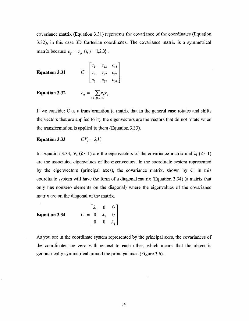
covariance matrix (Equation 3.31) represents the covariance of the coordinates (Equation
3.32), in this case 3D Cartesian coordinates. The covariance matrix is a symmetrical
matrix because cy = c 7 {/, j = 1,2,3}.
Equation 3.31
Equation 3.32
C = cn cn cu
c3l c 3 2 c3 3
C8= TX'XJ rj={l,2,3}
If we consider C as a transformation (a matrix that in the general case rotates and shifts
the vectors that are applied to it), the eigenvectors are the vectors that do not rotate when
the transformation is applied to them (Equation 3.33).
Equation 3.33 cv, = xy,
In Equation 3.33, Vj (i>=l) are the eigenvectors of the covariance matrix and \\ (i>=l)
are the associated eigenvalues of the eigenvectors. In the coordinate system represented
by the eigenvectors (principal axes), the covariance matrix, shown by C in this
coordinate system will have the form of a diagonal matrix (Equation 3.34) (a matrix that
only has nonzero elements on the diagonal) where the eigenvalues of the covariance
matrix are on the diagonal of the matrix.
Equation 3.34 C' = X o 0 A,
0
0
0 0 A,
As you see in the coordinate system represented by the principal axes, the covariances of
the coordinates are zero with respect to each other, which means that the object is
geometrically symmetrical around the principal axes (Figure 3.6).
34

Figure 3.6 - Object is geometrically symmetrical around the principal axes (x'i, x'2,
x'3)
A closer look at C" shows that the eigenvalues are in fact the variances of the coordinates
of the object points (segmentation pixels) in the principal coordinate system. We define
the Principal Axis Difference comparison measure as follows:
Equation 3.35 PAD - abs(abs(max(ljTS )) - abs(max(XiSUT ))) i - {1,2,3}
PAD is calculating the difference of the largest variance of the pixels along the principal
axes of the true segmentation and the segmentation under test. PAD solely concentrates
on the shape of the segmentations and thus if the shape of the segmentation under test is
the same as the true segmentation PAD would depict no difference between the
segmentations, this is while the labeling in the segmentation under test may be located at
a different location in the image from the expected location, making it an incorrect
segmentation.
3.1.2.8 RMS surface distance
The RMS surface distance is defined as follows [17]:
Equation 3.36 RMSSD = z
I psbd(SUT)
min d(p,q) qebd(TS) qebd(TS)
~\2
min d(q, p) pEbd(SUT)
bd(SUT) I +1 bd(TS) \
35
RMSSD (Root Mean Square Surface Distance) is effectively taking a root mean square
type average of the distances between the boundary (surface) pixels of the segmentation
under test and the true segmentation over all the boundary pixels of both segmentations.
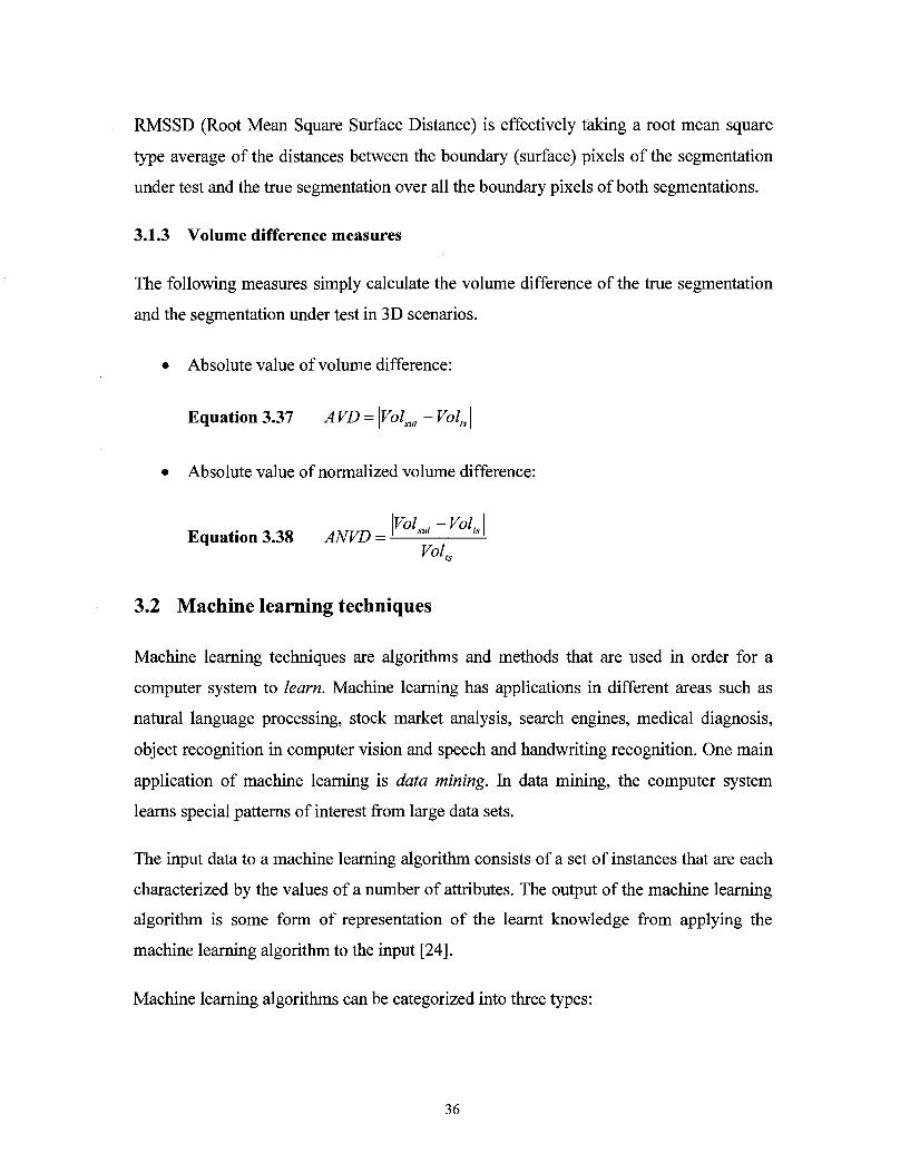
3.1.3 Volume difference measures
The following measures simply calculate the volume difference of the true segmentation
and the segmentation under test in 3D scenarios.
• Absolute value of volume difference:
Equation 3.37 AVD = \Volsut -Volts\
• Absolute value of normalized volume difference:
Vol „t-Vol' Equation 3.38 ANVD =
Slit tS\
Vol ts
3.2 Machine learning techniques
Machine learning techniques are algorithms and methods that are used in order for a
computer system to learn. Machine learning has applications in different areas such as
natural language processing, stock market analysis, search engines, medical diagnosis,
object recognition in computer vision and speech and handwriting recognition. One main
application of machine learning is data mining. In data mining, the computer system
learns special patterns of interest from large data sets.
The input data to a machine learning algorithm consists of a set of instances that are each
characterized by the values of a number of attributes. The output of the machine learning
algorithm is some form of representation of the learnt knowledge from applying the
machine learning algorithm to the input [24].
Machine learning algorithms can be categorized into three types:
36

1) Classification algorithms: These algorithms associate a class to an unknown
instance (i.e. an instance which the associated class is not known.). These are the
type of algorithms that we are interested in, in this thesis.
2) Association algorithms: These algorithms find associations between the attributes
that characterize the instances.
3) Clustering: These algorithms divide the instances into natural groups.
We will only concentrate on classification algorithms in this thesis. A classification
algorithm is trained via instances that have known classifications (training instances) to
create a model that can predict the class of unknown instances. This learnt model is
referred to as a classifier.
Some important categories of classification algorithms are as follows:
1) Rule-induction techniques: In these methods the classifier is represented by a set
of rules that each associate a particular class to a certain relationship among the
attributes.
2) Decision Trees: A divide-and-conquer approach is taken to construct a decision
tree for classifying instances.
3) Probabilistic models: These models output the probability that each instance can
belong to each class. The instance will be classified to the class with the highest
probability.
4) Linear Models: A weighted linear function is learnt by solving an optimization
problem. This linear function is used to classify unknown instances.
5) Instance-based learning: In this technique, the training instances are stored
verbatim and methods such as finding the nearest neighbor are used to find the
nearest training instance to the unknown instance, in which case the unknown
instance is predicated to have the same class as the nearest training instance [24].
37
Decision trees and rule induction techniques are of particular interest as their models are
readily interpretable by experts using them. The learnt model (classifier), output from the
machine learning algorithm, has to be validated. In machine learning systems, the input
data is divided into two main sets: the training set and the test set. The training set is used
to construct the model and the test set is used to validate the model. Validating the model
by deriving the error rate using the training model itself would lead to very optimistic
results. Thus the test set should preferably be independent of the training set. Both the
training and test sets should have representative instances of all types in the underlying
problem so that the model is thorough and the validation of the model is also
comprehensive. One of the techniques used to guarantee that all the representative
samples are taken into account in the training or test sets is referred to as stratification.
Stratification attempts to randomly choose the instances such that all the classes (that
each of the instances belongs to) are represented in the right proportion, i.e., no class is
over-represented by too many samples or under-represented by scarce samples. In an
effort towards finding a reasonable error estimate to validate the model, a method
referred to as cross-validation is commonly used. In this method, the available data is
divided into a number of folds, each time one fold is used as the test set and the
remainder is used for the training data. The cross-validation error estimate is the average
of the error estimates that are calculated using each fold. Each error estimate could be
simply the division of the number of misclassified test instances by the total number of
test instances. Usually stratification is also used in cross-validation. For example, a 10-
fold cross-validation along with stratification is referred to as stratified 10-fold cross-
validation which is usually the standard way of measuring the error rate of a learning
method. In order to reduce any bias towards choosing the training and test set instances it
is common to repeat stratified 10-fold cross-validation 10 times and get the average of the
error estimates obtained from each cross-validation run. Other error estimates such as
leave-one-out cross-validation are also used. In this approach each time one instance is
left out for testing while the rest of the instances are used for training. This approach is
repeated until all of the instances are used once for testing the learning method. Leave-
one-out cross-validation does not involve any stratification as it uses the whole data set
for both training and testing purposes, and is therefore computationally expensive.
38
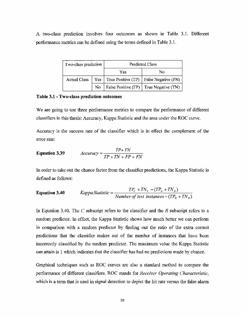
A two-class prediction involves four outcomes as shown in Table 3.1. Different
performance metrics can be defined using the terms defined in Table 3.1.
Two-class prediction
Actual Class Yes
No
Predicted Class
Yes
True Positive (TP)
False Positive (FP)
No
False Negative (FN)
True Negative (TN)
Table 3.1 - Two-class prediction outcomes
We are going to use three performance metrics to compare the performance of different
classifiers in this thesis: Accuracy, Kappa Statistic and the area under the ROC curve.
Accuracy is the success rate of the classifier which is in effect the complement of the
error rate:
Equation 3.39 Accuracy = TP+TN
TP + TN + FP + FN
In order to take out the chance factor from the classifier predictions, the Kappa Statistic is
defined as follows:
Equation 3.40 Kappa Statistic = TPC+TNC-(TPR+TNR)
Number of test instances - (TPR + TNR )
In Equation 3.40, The C subscript refers to the classifier and the R subscript refers to a
random predictor. In effect, the Kappa Statistic shows how much better we can perform
in comparison with a random predictor by finding out the ratio of the extra correct
predictions that the classifier makes out of the number of instances that have been
incorrectly classified by the random predictor. The maximum value the Kappa Statistic
can attain is 1 which indicates that the classifier has had no predictions made by chance.
Graphical techniques such as ROC curves are also a standard method to compare the
performance of different classifiers. ROC stands for Receiver Operating Characteristic,
which is a term that is used in signal detection to depict the hit rate versus the false alarm
39
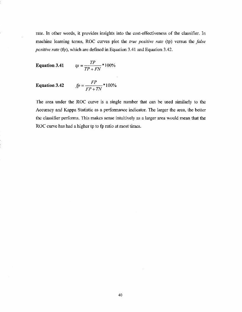
rate. In other words, it provides insights into the cost-effectiveness of the classifier. In
machine learning terms, ROC curves plot the true positive rate (tp) versus the false
positive rate (fp), which are defined in Equation 3.41 and Equation 3.42.
TP Equation 3.41 tp = * 100%
TP + FN
Equation 3.42 fp = F? * 100% Jy FP + TN
The area under the ROC curve is a single number that can be used similarly to the
Accuracy and Kappa Statistic as a performance indicator. The larger the area, the better
the classifier performs. This makes sense intuitively as a larger area would mean that the
ROC curve has had a higher tp to fp ratio at most times.
40
4 IMAGE SEGMENTATION EVALUATION
ORACLE DESIGN
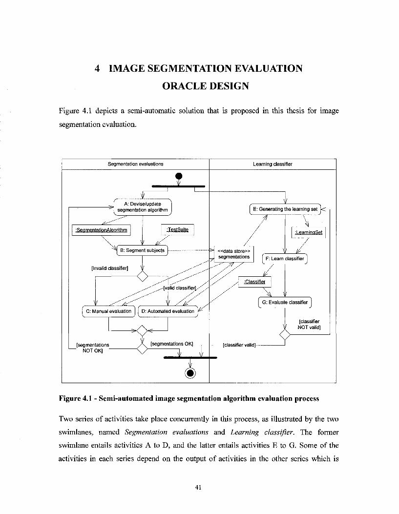
Figure 4.1 depicts a semi-automatic solution that is proposed in this thesis for image
segmentation evaluation.
Segmentation evaluations Learning classifier
i JL
-2H A: Devise/update
segmentation algorithm JL
E: Generating the learning set HS
s.-" :SeamentationAlaorithm TestSuite
1 £L B: Segment subjects
[invalid classifier] -54
H «data store» segmentations
JL :LearninaSet
1 £_ F: Learn classifier
--[valid classifier!.--:Classifier
J/ G: Evaluate classifier
[classifier NOT valid]
[segmentations " NOT OK]
[classifier valid]-
Figure 4.1 - Semi-automated image segmentation algorithm evaluation process
Two series of activities take place concurrently in this process, as illustrated by the two
swimlanes, named Segmentation evaluations and Learning classifier. The former
swimlane entails activities A to D, and the latter entails activities E to G. Some of the
activities in each series depend on the output of activities in the other series which is
41
further explained below (e.g., activity E takes an input produced by activity B, activity D
takes an input produced by activity F). In the left swimlane (the Segmentation evaluations
swimlane), the image segmentation algorithm is revised (activity A) and the
segmentations produced by each revision of the image segmentation algorithm (activity
B) are evaluated for their correctness. These are evaluated either manually by experts
(activity C) or automatically—see below (activity D). In the right swimlane (the Learning
classifier swimlane), a classifier is learnt. Once a valid classifier is learnt, the
segmentation evaluation in the evaluation thread is done automatically (activity D). These
two series of activities are further described below in Sections 4.1 and 4.2, respectively.
We then discuss the architecture of our tool support in Section 4.3.
4.1 Segmentation evaluations swimlane
This swimlane has four activities: activities A to D. The first time the Devise/Update
segmentation algorithm activity (Activity A) is performed, an initial version of the image
segmentation algorithm is devised. Each time this activity is repeated, i.e., when the
overall evaluation of the segmentations produced by the image segmentation algorithm
fails, the image segmentation algorithm is revised. Further revisions of the image
segmentation algorithm are made in subsequent iterations until a satisfactory set of
segmentations are produced by a revision of the image segmentation algorithm.
During the Segment subjects activity (Activity B), the segmentation algorithm produced
in activity A is used to segment a set of sample subject images or test cases (input named
Test suite). This results in a set of segmentations, each segmentation corresponding to
one sample subject (test case). We refer to the segmentations obtained from revision i of
the segmentation algorithm (i.e., during the i* iteration of this swimlane) as segmentation
set sett.
The segmented images are evaluated either manually or automatically in the next two
activities (C and D), depending on whether a valid classifier has been learnt. If a valid
classifier has not yet been learnt (Section 4.2), the segmentations have to be manually
evaluated (Activity C—Manual evaluation of segmentations). Each segmentation is
graded by both the image segmentation algorithm designer and medical experts and is
42
considered as correct if it receives a reasonable grade (The grading scale is to be decided
by the algorithm designer and the medical expert.). If a valid classifier is available
(Section 4.2), the evaluation is done automatically: activity Automated evaluation of
segmentations (Activity D). In this case, the classifier predicts the grade of each
segmentation without the intervention of a human expert (algorithm designer or medical
expert). During automated evaluation, segmentations produced by the current revision (i)
of the segmentation algorithm are compared by the classifier (using similarity measures)
to segmentations produced by the previous revisions (j<i) of the segmentation algorithm.
The details of how this is done are explained in Section 4.3.
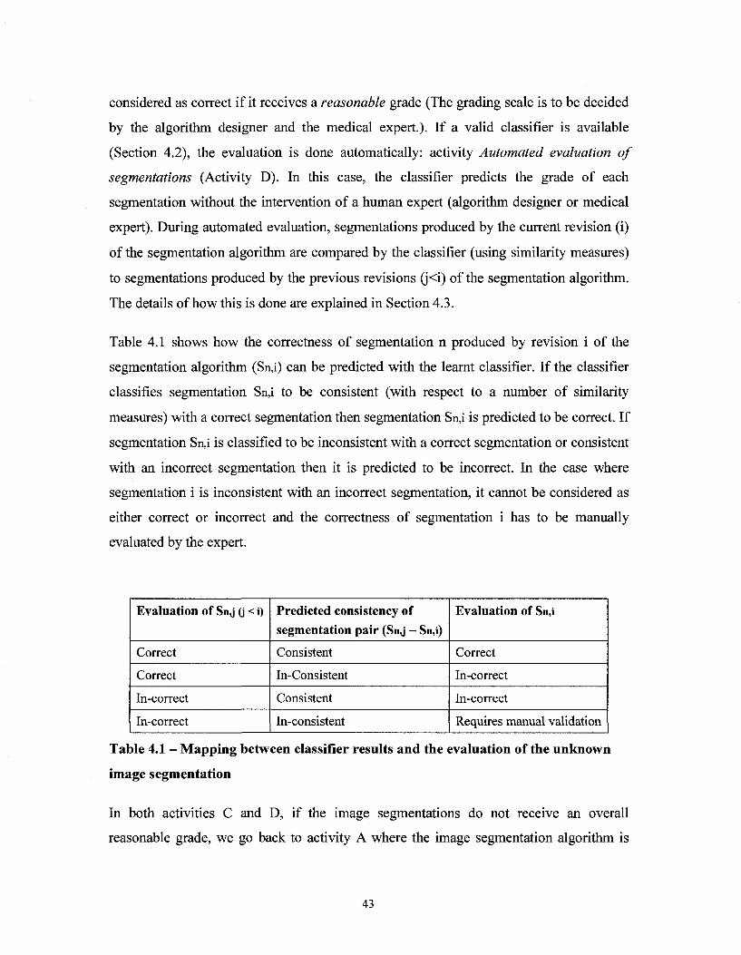
Table 4.1 shows how the correctness of segmentation n produced by revision i of the
segmentation algorithm (Sn,i) can be predicted with the learnt classifier. If the classifier
classifies segmentation Sn,i to be consistent (with respect to a number of similarity
measures) with a correct segmentation then segmentation Sn,i is predicted to be correct. If
segmentation Sn,i is classified to be inconsistent with a correct segmentation or consistent
with an incorrect segmentation then it is predicted to be incorrect. In the case where
segmentation i is inconsistent with an incorrect segmentation, it cannot be considered as
either correct or incorrect and the correctness of segmentation i has to be manually
evaluated by the expert.
Evaluation of Sn,j (j < i)
Correct
Correct
In-correct
In-correct
Predicted consistency of segmentation pair (Sn,j - Sn,i)
Consistent
In-Consistent
Consistent
In-consistent
Evaluation of Sn,i
Correct
In-correct
In-correct
Requires manual validation
Table 4.1 - Mapping between classifier results and the evaluation of the unknown
image segmentation
In both activities C and D, if the image segmentations do not receive an overall
reasonable grade, we go back to activity A where the image segmentation algorithm is
43
revised. Otherwise, the testing process ends and the current revision of the image
segmentation algorithm is deemed to be correct.
The idea of using multiple versions of the segmentation algorithm to find out whether the
output of the segmentation algorithm is correct is similar to multi-version programming
mentioned in Chapter 2. Note that in our case the multiple versions are a natural result of
the evolution of the software until an acceptable version is devised, so the cost involved
in producing extra versions of the same software that are solely for testing purposes is not
applicable in our methodology.
4.2 Learning classifier swimlane
This swimlane has three activities: activities E to G. During Activity E (Generating the
learning set), pairs of segmentations obtained from multiple revisions of the image
segmentation algorithm (current revision i, and revision j,j<i) are compared using a set of
similarity measures (Section 3.1). At least the first two sets of segmentations generated
by the first two revisions of the segmentation algorithm are required to get the first set of
similarity measurements (i.e., the first set of evaluated segmentation pairs from versions
1 and 2 of the segmentation algorithm). In other words, at least two iterations of the
Segmentation evaluations swimlane (with manual evaluation in Activity C) are
necessary.
Pairing segmentations of the same subjects across two segmentation sets sett and setj
results in three distinct subsets of paired segmentations. The first set is composed of the
pairs of segmented subjects that were both deemed correct by an expert, denoted by setyy
(i.e., 'y' for "yes" for the two versions). The second set is composed of the pairs of
segmented subjects where either the first or second segmented subject was deemed
incorrect, denoted by setyn (one is correct, i.e., one 'y', and one is incorrect, i.e., one 'n').
The third set is the set of all the pairs of segmented subjects that were both considered
incorrect, denoted by setnn.
The learning algorithm (Activity F) does not use setnn as the information obtained from
comparing two incorrectly segmented subjects would not help the learning algorithm
44

construct a classifier to recognize diagnostically equivalent segmentations. Two
segmentations may be incorrect for two completely different reasons and thus we cannot
categorize them as consistent with each other. Table 4.2 explains how we categorize a
pair of segmentations to be consistent\inconsistent where Sn,i and Snj are two
segmentations obtained from subject n using versions i and j of the segmentation
algorithm, respectively.
Similarity measures (Section 3.1) are used to compare the paired segmented subjects in
sets setyy and setyn. In other words, for each pair of segmentation algorithms applied to the
same set of subjects, Activity E generates a set of tuples with a size equal to the number
of subjects considered: (smn, ..., sniik, Consistency), where smy denotes similarity
measure j on subject pair i and "Consistency" can take two values: yy or yn. k is the
number of similarity measures.
Manual evaluation of Sn,i
Correct
Correct
Incorrect
Incorrect
Manual evaluation of Sn,j
Correct
Incorrect
Correct
Incorrect
Class
Consistent
Inconsistent
Inconsistent
Unusable (not a class)
Table 4.2 - Consistency of two segmentations
This set of tuples is the training set of instances that is fed into the machine learning
algorithm: activity F (Learn classifier). The machine learning algorithm learns which
ranges of these measures, and which of these measures, correspond to a diagnostically
consistent pair of segmentations, and which ranges (and measures) correspond to a
diagnostically inconsistent pair of segmentations. A diagnostically consistent pair of
segmentations refers to two segmentations that both lead to the same diagnostic by the
expert (algorithm designer or medical expert).
The learnt classifier (activity F) is validated using techniques such as 10-fold cross-
validation (Section 3.2) in activity G (Evaluate classifier). A classifier is deemed valid if
the average error estimate is considered to be sufficiently low to be used in practice. This
45

means that the classifier correctly predicted a reasonable proportion of segmentations
under test to be consistent or inconsistent with a reference segmentation of the same
subject, or in other words predicted if the segmentation under test is correct or not. Once
the classifier is learnt, the evaluation in the Segmentation evaluations swimlane can be
done automatically (activity D). In the case where we do not succeed in learning a
classifier with very high accuracy, there are always some branches (in the case of
decision trees) or rules (in the case of rule induction techniques) where the classifier has a
very low error rate and its predictions can be trusted with high confidence. If the
classifier can provide accurate predictions for a significant number of cases, then the
classifier is a good candidate for automatic evaluation.
4.3 Tool support architecture
The structural components in the design of the automated oracle are shown in Figure 4.2.
As shown in Figure 4.2, the oracle design is generic and does not have to be restricted to
the image segmentation evaluation domain. The outputs (in our case the segmentations)
from version Vi (1 < / < n where n is the total number of versions of the Software Under
Test (SUT) until its depicted as valid) of the software under test (in our case the software
under test is the segmentation algorithm) are fed into the oracle and the oracle determines
the correctness of the outputs.
46
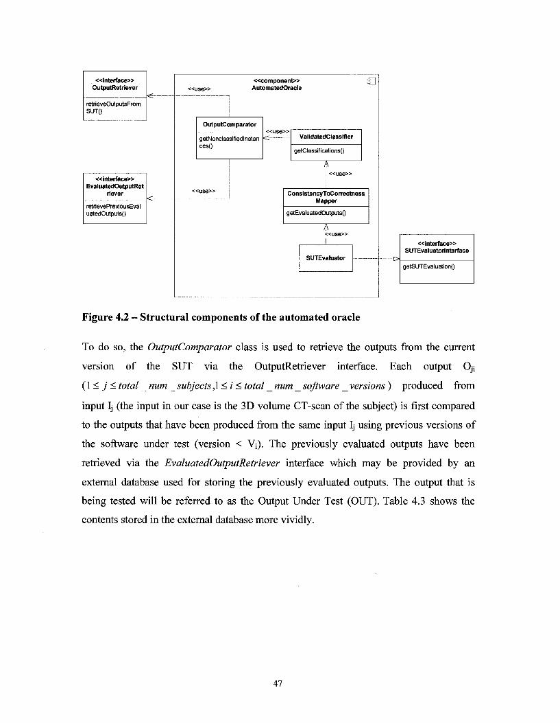
«interface» OutputRetriever
retrieveOutputsFrom SUT()
L ^ „
«interface» EvaluatedOutputRet
retrievePreviousEval uatedOutputs()
K
«componerrt» AutomatedOracle a
OutputComparator « u s e »
getNonclassifiedlnstan | < ces()
ValidatedClassifier
getClassificationsQ
T"
ConsistencyToCorrectness Mapper
getEvaluatedOutputsQ
"J « u s e »
SUTEvaluator
Figure 4.2 - Structural components of the automated oracle
«interface» SUTEvaluator! nterface
getSUTEvaluation()
To do so, the OutputComparator class is used to retrieve the outputs from the current
version of the SUT via the OutputRetriever interface. Each output Oji
(1 < j < total _ num _ subjects ,1 < / < total _ num _ software _ versions ) produced from
input Ij (the input in our case is the 3D volume CT-scan of the subject) is first compared
to the outputs that have been produced from the same input Ij using previous versions of
the software under test (version < Vi). The previously evaluated outputs have been
retrieved via the EvaluatedOutputRetriever interface which may be provided by an
external database used for storing the previously evaluated outputs. The output that is
being tested will be referred to as the Output Under Test (OUT). Table 4.3 shows the
contents stored in the external database more vividly.
47
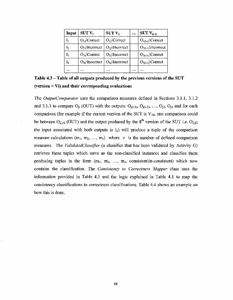
Input
I,
h
h
u
SUTVi
On\Correct
02i\Incorrect
03i\Correct
04i\Incorrect
SUTV2
OnXCorrect
022\Incorrect
032\Incorrect
042\Incorrect
... SUTV(i.D
Oi(i.i)\Correct
02(i-i)\Incorrect
03(i.i)\Correct
04(i.i)\Correct
Table 4.3 - Table of all outputs produced by the previous versions of the SUT
(version < Vi) and their corresponding evaluations
The OutputComparator uses the comparison measures defined in Sections 3.1.1, 3.1.2
and 3.1.3 to compare Oji (OUT) with the outputs: Oj(i-i), Oj(i_2), ..., Oj2, Oji and for each
comparison (for example if the current version of the SUT is Vio, one comparison could
be between C^jo (OUT) and the output produced by the 8th version of the SUT i.e. 02,s;
the input associated with both outputs is I2) will produce a tuple of the comparison
measure calculations (mi, ni2, ..., mz) where z is the number of defined comparison
measures. The ValidatedClassifier (a classifier that has been validated by Activity G)
retrieves these tuples which serve as the non-classified instances and classifies them
producing tuples in the form (mi, ni2, ..., mz, consistent\in-consistent) which now
contains the classification. The Consistency to Correctness Mapper class uses the
information provided in Table 4.3 and the logic explained in Table 4.1 to map the
consistency classifications to correctness classifications. Table 4.4 shows an example on
how this is done.
48
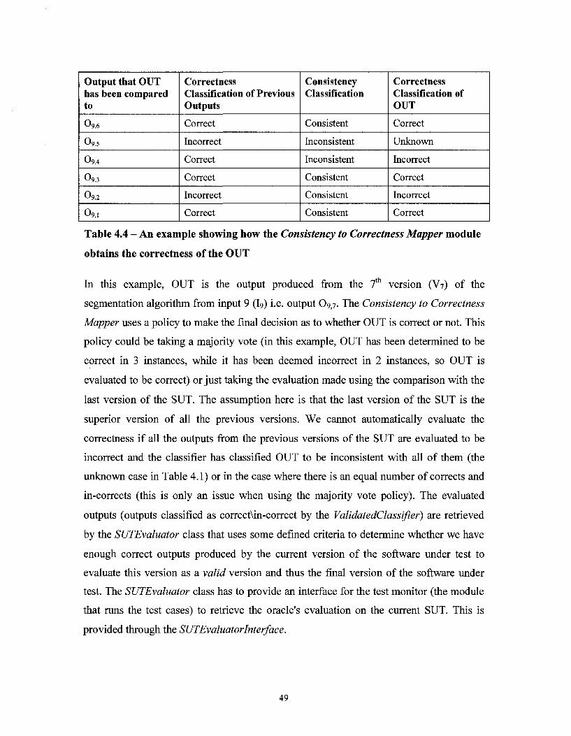
Output that OUT has been compared to
09.6
0 9 5
09.4
0 9 3
O9.2
09 , i
Correctness Classification of Previous Outputs
Correct
Incorrect
Correct
Correct
Incorrect
Correct
Consistency Classification
Consistent
Inconsistent
Inconsistent
Consistent
Consistent
Consistent
Correctness Classification of OUT
Correct
Unknown
Incorrect
Correct
Incorrect
Correct
Table 4.4 - An example showing how the Consistency to Correctness Mapper module
obtains the correctness of the OUT
In this example, OUT is the output produced from the 7 version (V7) of the
segmentation algorithm from input 9 (I9) i.e. output O97. The Consistency to Correctness
Mapper uses a policy to make the final decision as to whether OUT is correct or not. This
policy could be taking a majority vote (in this example, OUT has been determined to be
correct in 3 instances, while it has been deemed incorrect in 2 instances, so OUT is
evaluated to be correct) or just taking the evaluation made using the comparison with the
last version of the SUT. The assumption here is that the last version of the SUT is the
superior version of all the previous versions. We cannot automatically evaluate the
correctness if all the outputs from the previous versions of the SUT are evaluated to be
incorrect and the classifier has classified OUT to be inconsistent with all of them (the
unknown case in Table 4.1) or in the case where there is an equal number of corrects and
in-corrects (this is only an issue when using the majority vote policy). The evaluated
outputs (outputs classified as correct\in-correct by the ValidatedClassifier) are retrieved
by the SUTEvaluator class that uses some defined criteria to determine whether we have
enough correct outputs produced by the current version of the software under test to
evaluate this version as a valid version and thus the final version of the software under
test. The SUTEvaluator class has to provide an interface for the test monitor (the module
that runs the test cases) to retrieve the oracle's evaluation on the current SUT. This is
provided through the SUTEvaluator Interface.
49

5 CASE STUDY: LEFT HEART VENTRICLE
SEGMENTATION EVALUATION
The case study that is used in this research work is evaluating the correctness of the
segmentation algorithms that are devised to segment the left heart ventricle. Once the left
ventricle is identified, its volume is computed for diagnostic purposes; this is however not
in the scope of this thesis. Before we start talking about the details of the case study and
how we have used the solution proposed in Chapter 4 to solve the problem of evaluating
medical image segmentations in a timely fashion we explain why the software under test
(the medical image segmentation algorithms) can be considered as un-testable programs
with a discussion based on the three criteria given for un-testable programs in [1] (refer to
Chapter 2).
In order to verify the correctness of a devised medical image segmentation algorithm, the
segmentation algorithm is applied to a sample subset of subjects; if a predefined
percentage of the output segmentations are deemed to be correct, the segmentation
algorithm is deemed correct. A medical expert can manually segment a subject, so the
output of the segmentation algorithm is known, but it is very dependent on the
availability of the medical expert and is very time-consuming considering the large size
of the sample test-set. Typically, hundreds of subjects are used. As the correct
segmentation is usually not available we can consider the output of the segmentation
algorithm to be "unknown" (category 1 of untestable software described in Chapter 2).
The process of devising the final segmentation algorithm is an iterative process requiring
many revisions of the initial segmentation algorithm. As the same medical experts are not
always available during the evaluation of the image segmentation algorithm, different
versions of the image segmentation algorithm may be evaluated by different medical
experts. This leads to subjectivity in the overall assessment of the quality of each version
of the image segmentation algorithm as different experts may impose different weights to
different aspects of their assessment. This implicitly indicates the segmentation algorithm
50
is being evaluated with respect to (slightly) different specifications (the oracle problem is
in category 3 of untestable software described in Chapter 2).
Considering the problem of testing the correctness of medical image segmentation
algorithms lies in categories 1 and 3, in the context explained in [1] we could refer to the
medical segmentation algorithm as an untestable program. In this case study we tackle
the problem of testing medical image segmentation algorithms using the approach
defined in chapter 4. In this approach we only need medical expert intervention for the
first few revisions of the segmentation algorithm (two revisions proves to be enough in
this case study), which partly relieves the problem of having a large dependency on the
medical experts to evaluate each and every revision of the segmentation algorithm
because of lack of knowledge of what the correct segmentation for each subject is
(category 1). If we get the majority vote of the medical experts in the evaluation of the
first few revisions of the segmentation algorithm, we do not encounter subjectivity in the
evaluation of the different revisions of the segmentation algorithm as the evaluation is
done automatically based on the majority vote done for the first few revisions and does
not depend on a possibly different medical expert's evaluation for different revisions of
the segmentation algorithm (category 3).
This chapter is divided into 9 sections. In order to give the reader a better idea about the
left heart ventricle segmentation, some segmentations are shown in Section 5.1. Section
5.2 details the setup of the experiments. In order to give some insight into how the
classification algorithms used in this thesis work, the three main data mining techniques
used in this case study (J48, PART and JRIP) are described in Section 5.3. Section 5.4
describes how the defined attributes (comparison measures) are correlated using
Spearman coefficients. The different attribute sets used for training the classifiers and the
reasoning behind choosing them is explained in Section 5.5. Section 5.6 shows the
classifiers output from the data mining techniques and explains how to interpret them.
The performance of the classifiers is compared in Section 5.7 using metrics such as
Accuracy, Kappa Statistic and the area under the ROC curve. The analysis and
implementation tools used in this case study are described in Section 5.8 explaining their
51
pros and cons. A discussion of the calculation time of the different types of comparison
measures is given in Section 5.9 concluding the chapter in Section 5.10.
5.1 Examples
We show here some figures showing the left heart ventricle segmentations. Each figure is
a slice of the CT-Scan of a different patient's heart where the left ventricle is segmented
by labeling the representative pixels with green using some version of the segmentation
algorithm. Figure 5.1 shows a correct segmentation while Figures Figure 5.2, Figure 5.3
and Figure 5.4 show incorrect segmentations. Figure 5.2 shows a typical
oversegmentation scenario (the most common problem in this case study) where the left
atrium is also labeled. In Figure 5.3 the segmentation algorithm has missed the left
ventricle and labeled the right ventricle instead. Severe undersegmentation is seen in
Figure 5.4 where almost nothing is labeled in this slice of the heart. These are some
examples of incorrect segmentations in this case study. More detailed discussion on the
manual evaluation of each segmentation is out of the context of this research work and
requires background in the heart anatomy. Also note that these figures only outline the
segmented region in one slice of the heart. In order to evaluate the correctness of a
segmentation, all the CT-Scan slices of the heart have to be looked at by an expert where
an overall assessment is then given as to whether the segmentation is correct or not.
Minor discrepancies in a few slices may be ignored by the expert. As explained earlier
the tolerance level for accepting a segmentation as correct may be different for each
expert.
52
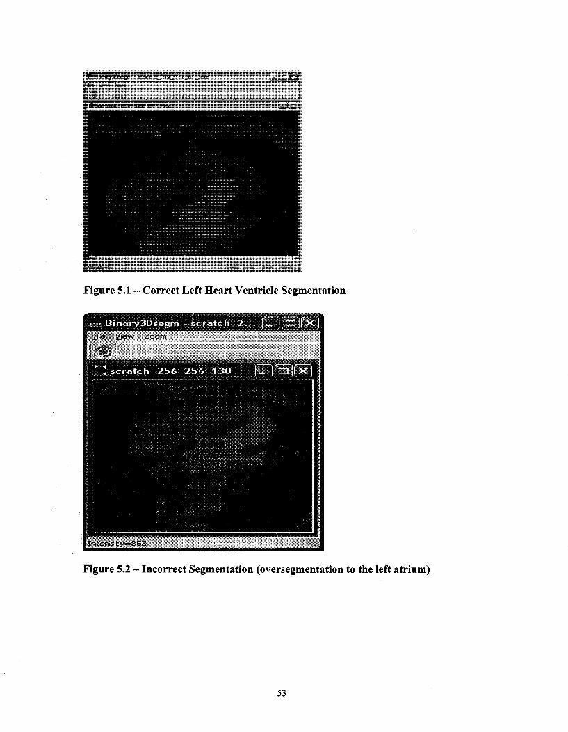
* Bin/tryTOsiuyri sr.rdlr.h_51 ?_"i1 ? fi1. .ritwt
F |i» i>w Zoom
Figure 5.1 - Correct Left Heart Ventricle Segmentation
:iw B inary3D^eg i r r - sc ra t c
Figure 5.2 - Incorrect Segmentation (oversegmentation to the left atrium)
53
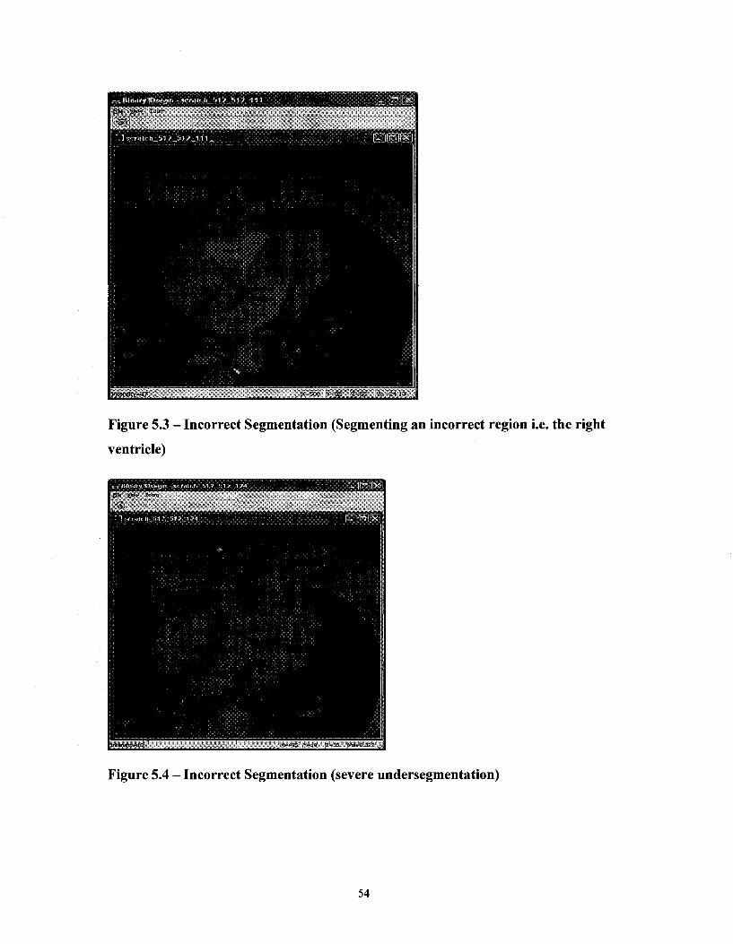
ra tch_512_512„ l11 .
'•71 «- | . l t r .h_S1/_M^_111_ tJfnJfEJ
Figure 5.3 - Incorrect Segmentation (Segmenting an incorrect region i.e. the right
ventricle)
X-"t95~ Y-19 *Z=35~ Mft-0.327
Figure 5.4 - Incorrect Segmentation (severe undersegmentation)
54

5.2 Experiment setup
Table 5.1 summarizes the details of the case study. CT-Scan images of the heart of 50
patients have been taken at different phases of the cardiac cycle. Each phase is a point of
time in the cardiac cycle. At each phase, the 3D volume of the heart is represented by a
set of 2D CT-Scan images obtained from the heart in that phase (in this case study, this
set could have from 53 to 460 images). Each of the 2D CT-Scan images depicts either a
256 by 256 or 512 by 512 pixel slice of the heart represented in the DICOM (Digital
Imaging and Communication in Medicine) format, which is a standard file format for
representing medical images. The obtained 3D volume of the heart in each phase
constitutes a test case or subject (181 in this case study).
Segmentation Target
Number of patients
Number of test cases in test suite
Number of attributes (measures)
Number of positive instances
Comparison measure types
Machine learning algorithms
Classifier evaluation technique
Performance Metrics
Left ventricle of the heart
50
181
18
104
Overlap, Volume Difference, Geometrical
C4.5, JRIP, PART
Stratified 10-fold cross-validation
Accuracy, Kappa Statistic, Area under ROC curve
Table 5.1 - Details of case study
Two revisions of the image segmentation algorithm have been used to obtain two sets of
image segmentations of the subjects. The image segmentations have been manually
evaluated by the author of this writing with the help of Siemens Corporate Research
experts (Activity C in Chapter 4). The grading scheme is a binary grading scheme; an
image segmentation is either evaluated as correct or incorrect. In order to generate the
training set (Activity E) for the machine learning algorithms, for each subject, the
segmentations produced by image segmentation algorithm versions 1 and 2 are compared
using different combinations of the comparison measures in Table 5.2 (please refer to
55
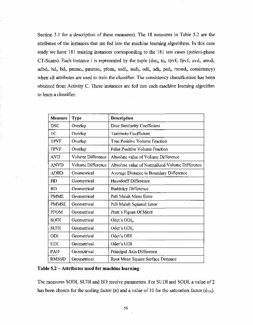
Section 3.1 for a description of these measures). The 18 measures in Table 5.2 are the
attributes of the instances that are fed into the machine learning algorithms. In this case
study we have 181 training instances corresponding to the 181 test cases (patient-phase
CT-Scans). Each instance i is represented by the tuple (dsc;, to;, tpvfi, fpvf;, avd;, anvd;,
adbdi, hdi, bdi, pmme;, pmrnse;, pfom;, sodi;, sudij, odi;, udi;, pad;, rmssd;, consistency)
when all attributes are used to train the classifier. The consistency classification has been
obtained from Activity C. These instances are fed into each machine learning algorithm
to learn a classifier.
Measure
DSC
TC
TPVF
FPVF
AVD
ANVD
ADBD
HD
BD
PMME
PMMSE
PFOM
SODI
SUDI
ODI
UDI
PAD
RMSSD
Type
Overlap
Overlap
Overlap
Overlap
Volume Difference
Volume Difference
Geometrical
Geometrical
Geometrical
Geometrical
Geometrical
Geometrical
Geometrical
Geometrical
Geometrical
Geometrical
Geometrical
Geometrical
Description
Dice Similarity Coefficient
Tanimoto Coefficient
True Positive Volume Fraction
False Positive Volume Fraction
Absolute value of Volume Difference
Absolute value of Normalized Volume Difference
Average Distance to Boundary Difference
Hausdorff Difference
Baddeley Difference
Peli Malah Mean Error
Peli Malah Squared Error
Pratt's Figure Of Merit
Odet's ODIn
Odet's UDIn
Odet's ODI
Odet's UDI
Principal Axis Difference
Root Mean Square Surface Distance
Table 5.2 - Attributes used for machine learning
The measures SODI, SUDI and BD receive parameters. For SUDI and SODI, a value of 2
has been chosen for the scaling factor (n) and a value of 10 for the saturation factor (dm)-
56
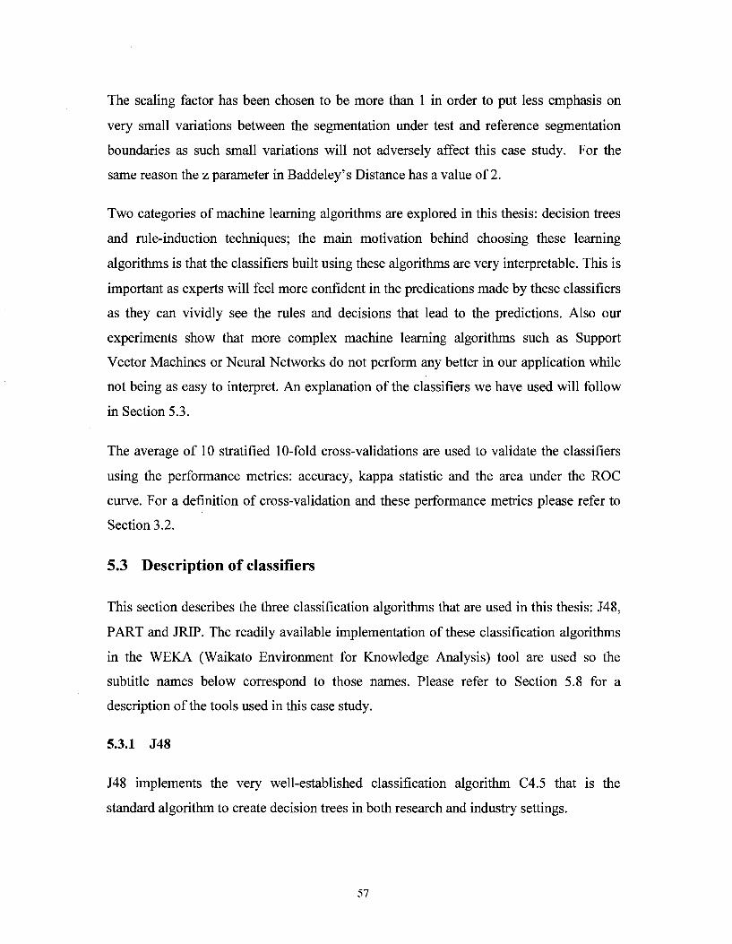
The scaling factor has been chosen to be more than 1 in order to put less emphasis on
very small variations between the segmentation under test and reference segmentation
boundaries as such small variations will not adversely affect this case study. For the
same reason the z parameter in Baddeley's Distance has a value of 2.
Two categories of machine learning algorithms are explored in this thesis: decision trees
and rule-induction techniques; the main motivation behind choosing these learning
algorithms is that the classifiers built using these algorithms are very interpretable. This is
important as experts will feel more confident in the predications made by these classifiers
as they can vividly see the rules and decisions that lead to the predictions. Also our
experiments show that more complex machine learning algorithms such as Support
Vector Machines or Neural Networks do not perform any better in our application while
not being as easy to interpret. An explanation of the classifiers we have used will follow
in Section 5.3.
The average of 10 stratified 10-fold cross-validations are used to validate the classifiers
using the performance metrics: accuracy, kappa statistic and the area under the ROC
curve. For a definition of cross-validation and these performance metrics please refer to
Section 3.2.
5.3 Description of classifiers
This section describes the three classification algorithms that are used in this thesis: J48,
PART and JRIP. The readily available implementation of these classification algorithms
in the WEKA (Waikato Environment for Knowledge Analysis) tool are used so the
subtitle names below correspond to those names. Please refer to Section 5.8 for a
description of the tools used in this case study.
5.3.1 J48
J48 implements the very well-established classification algorithm C4.5 that is the
standard algorithm to create decision trees in both research and industry settings.
57
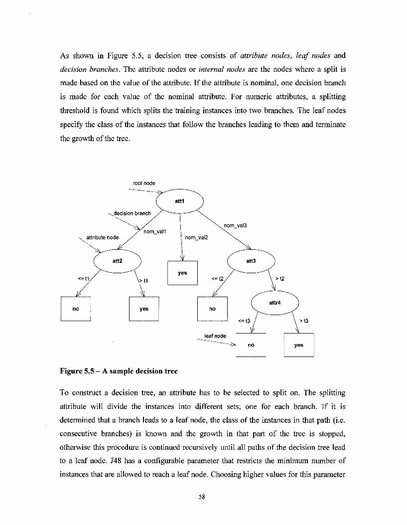
As shown in Figure 5.5, a decision tree consists of attribute nodes, leaf nodes and
decision branches. The attribute nodes or internal nodes are the nodes where a split is
made based on the value of the attribute. If the attribute is nominal, one decision branch
is made for each value of the nominal attribute. For numeric attributes, a splitting
threshold is found which splits the training instances into two branches. The leaf nodes
specify the class of the instances that follow the branches leading to them and terminate
the growth of the tree.
root node
Figure 5.5 - A sample decision tree
To construct a decision tree, an attribute has to be selected to split on. The splitting
attribute will divide the instances into different sets; one for each branch. If it is
determined that a branch leads to a leaf node, the class of the instances in that path (i.e.
consecutive branches) is known and the growth in that part of the tree is stopped,
otherwise this procedure is continued recursively until all paths of the decision tree lead
to a leaf node. J48 has a configurable parameter that restricts the minimum number of
instances that are allowed to reach a leaf node. Choosing higher values for this parameter
58
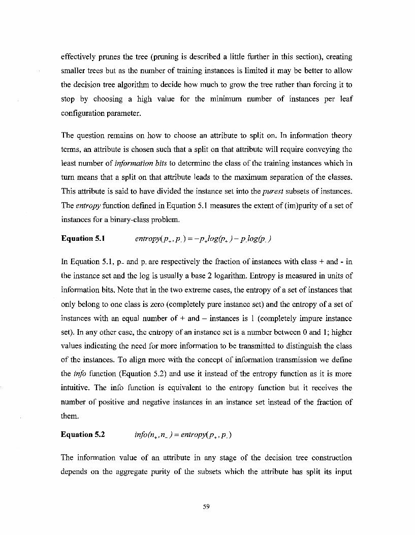
effectively prunes the tree (pruning is described a little further in this section), creating
smaller trees but as the number of training instances is limited it may be better to allow
the decision tree algorithm to decide how much to grow the tree rather than forcing it to
stop by choosing a high value for the minimum number of instances per leaf
configuration parameter.
The question remains on how to choose an attribute to split on. In information theory
terms, an attribute is chosen such that a split on that attribute will require conveying the
least number of information bits to determine the class of the training instances which in
turn means that a split on that attribute leads to the maximum separation of the classes.
This attribute is said to have divided the instance set into the purest subsets of instances.
The entropy function defined in Equation 5.1 measures the extent of (im)purity of a set of
instances for a binary-class problem.
Equation 5.1 entropy(p+ ,p.) = -pJog(p+ ) -p_log(p_)
In Equation 5.1, p+ and p. are respectively the fraction of instances with class + and - in
the instance set and the log is usually a base 2 logarithm. Entropy is measured in units of
information bits. Note that in the two extreme cases, the entropy of a set of instances that
only belong to one class is zero (completely pure instance set) and the entropy of a set of
instances with an equal number of + and - instances is 1 (completely impure instance
set). In any other case, the entropy of an instance set is a number between 0 and 1; higher
values indicating the need for more information to be transmitted to distinguish the class
of the instances. To align more with the concept of information transmission we define
the info function (Equation 5.2) and use it instead of the entropy function as it is more
intuitive. The info function is equivalent to the entropy function but it receives the
number of positive and negative instances in an instance set instead of the fraction of
them.
Equation 5.2 info(n+ ,n_) = entropy(p+ ,p_)
The information value of an attribute in any stage of the decision tree construction
depends on the aggregate purity of the subsets which the attribute has split its input
59
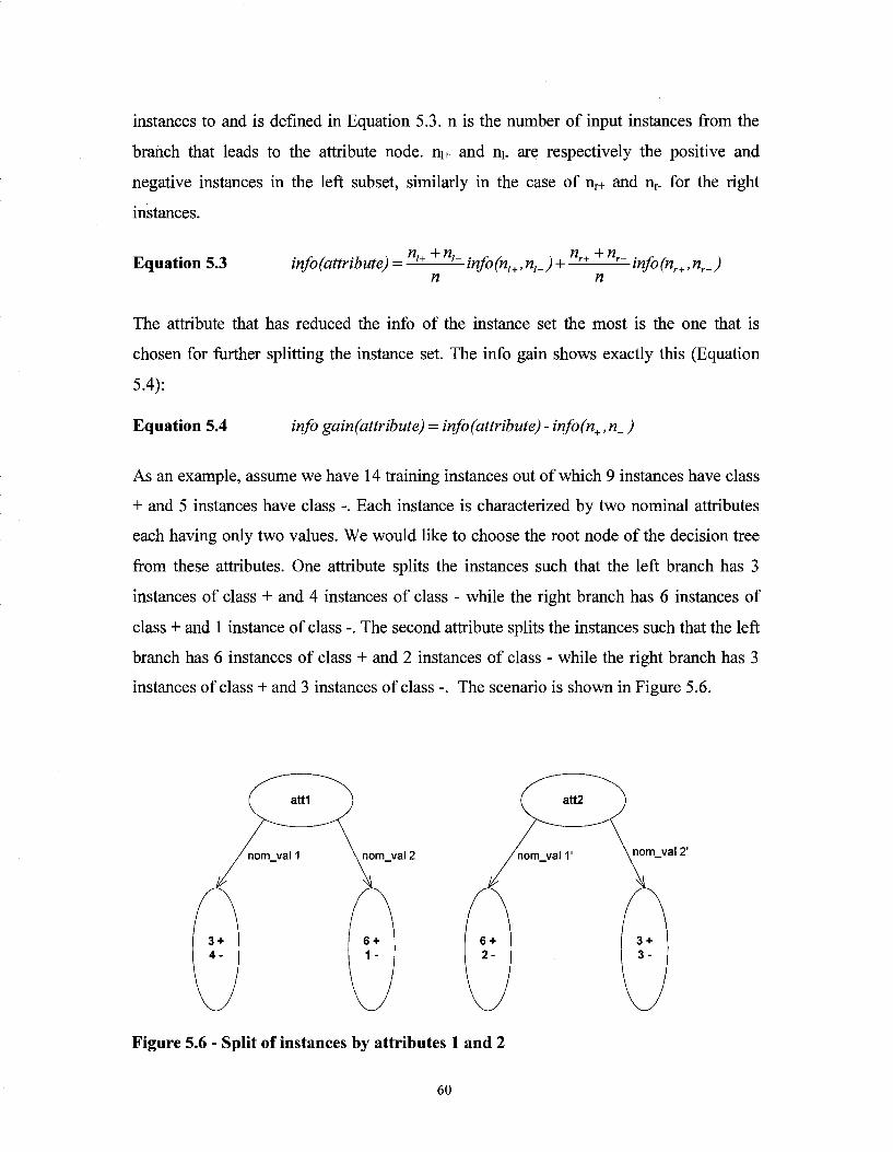
instances to and is defined in Equation 5.3. n is the number of input instances from the
branch that leads to the attribute node. ni+ and ni. are respectively the positive and
negative instances in the left subset, similarly in the case of n^ and nr. for the right
instances.
Yl ~}* Yl Yl ~h Yl
Equation 5.3 info (attribute) = —— —info(nl+,rii_ ) + -L± —info(nr+,nr_) n n
The attribute that has reduced the info of the instance set the most is the one that is
chosen for further splitting the instance set. The info gain shows exactly this (Equation
5.4):
Equation 5.4 info gain(attribute) = info (attribute) - info(n+, n_)
As an example, assume we have 14 training instances out of which 9 instances have class
+ and 5 instances have class -. Each instance is characterized by two nominal attributes
each having only two values. We would like to choose the root node of the decision tree
from these attributes. One attribute splits the instances such that the left branch has 3
instances of class + and 4 instances of class - while the right branch has 6 instances of
class + and 1 instance of class -. The second attribute splits the instances such that the left
branch has 6 instances of class + and 2 instances of class - while the right branch has 3
instances of class + and 3 instances of class -. The scenario is shown in Figure 5.6.
Figure 5.6 - Split of instances by attributes 1 and 2
60
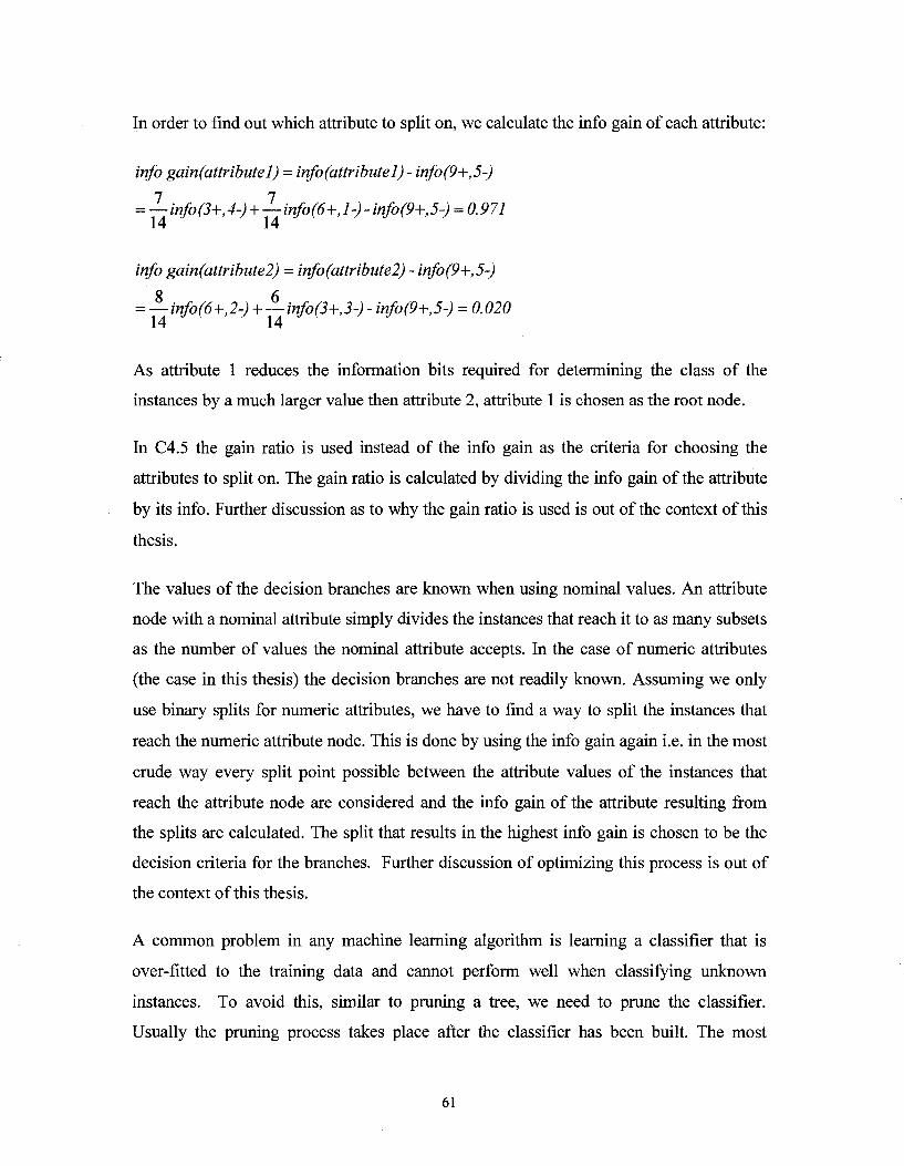
In order to find out which attribute to split on, we calculate the info gain of each attribute:
info gain(attributel) - info (attribute 1) - info(9+,5-)
=—info(3+,4-) +—info(6+,l-)-mfo(9+,5-) = 0.971
info gain(attribute2) = info (attribute!) - info(9+,5-)
= —info(6+,2-) + —info(3+,3-) - info(9+,5-) = 0.020
As attribute 1 reduces the information bits required for determining the class of the
instances by a much larger value then attribute 2, attribute 1 is chosen as the root node.
In C4.5 the gain ratio is used instead of the info gain as the criteria for choosing the
attributes to split on. The gain ratio is calculated by dividing the info gain of the attribute
by its info. Further discussion as to why the gain ratio is used is out of the context of this
thesis.
The values of the decision branches are known when using nominal values. An attribute
node with a nominal attribute simply divides the instances that reach it to as many subsets
as the number of values the nominal attribute accepts. In the case of numeric attributes
(the case in this thesis) the decision branches are not readily known. Assuming we only
use binary splits for numeric attributes, we have to find a way to split the instances that
reach the numeric attribute node. This is done by using the info gain again i.e. in the most
crude way every split point possible between the attribute values of the instances that
reach the attribute node are considered and the info gain of the attribute resulting from
the splits are calculated. The split that results in the highest info gain is chosen to be the
decision criteria for the branches. Further discussion of optimizing this process is out of
the context of this thesis.
A common problem in any machine learning algorithm is learning a classifier that is
over-fitted to the training data and cannot perform well when classifying unknown
instances. To avoid this, similar to pruning a tree, we need to prune the classifier.
Usually the pruning process takes place after the classifier has been built. The most
61

familiar pruning method in decision trees is subtree replacement where a subtree is
replaced by a leaf node. Other operations such as subtree raising are also used in C4.5
which we will not delve into more. A decision criterion has to be found to evaluate
whether this operation will actually improve the performance of the tree. To do so the
error rate of the tree before and after the subtree replacement operation is calculated and
if the error rate decreases the subtree is replaced by the majority class leaf node. If we use
the training data to calculate the error rate no pruning will ever take place as the error rate
will always increase after the pruning operation [24]. There are two ways to tackle this
problem.
One method is take a similar approach as cross-validation and divide the training data
into a number of folds using one fold for pruning and the other folds for training the
classifier. This is the approach taken in reduced-error pruning. In this way we make the
decision of whether to replace a subtree or not by comparing the error rate on the pruning
set which is independent of the training set. This approach has the obvious drawback of
reducing the number of instances used to train the data.
Another method is to use the training data, but this time instead of using the error rate
that is obtained from the classification of the pruning set before and after pruning, we
define our own error rate. The error rate here is the error that is introduced by replacing a
node with the majority class of the instances that reach that node i.e. the ratio of
misclassified instances as a result of the replacement to the total number of instances that
reach that node. As we are using the training instances, this error rate may be too
optimistic. Using the Bernoulli process to model the true error rate, we use the upper
confidence limit of the true error rate as our decision criteria for replacing a node which
takes away the optimism. We denote this error estimate as the C4.5 error estimate. To use
it, we first calculate the C4.5 error estimate for a parent node and then compare it with
the combined C4.5 error estimates of its leaf nodes (the leaf node error estimates are
combined in proportion with the ratio of the number of instances that reach each of
them). If the parent node C4.5 error estimate is lower, then pruning will take place. This
approach to pruning is proven to be effective in practice and is the default method of
pruning for the C4.5 classifier. We use C4.5 pruning for training the J48 classifier.
62

5.3.2 PART
PART is a rule-induction algorithm. Rule-induction algorithms take a covering approach
towards learning the classifier. In this approach, an attempt is made to construct a rule
that covers all the instances. Rule construction for the uncovered instances is continued
recursively until all the instances are covered by a rule.
PART uses partial decision trees to construct rules. It constructs a rule from the branch
leading to the leaf node that covers the most instances, thus creating the most general
rule. PART tries to avoid building a full decision tree for each rule. To do so, for every
attribute split, PART sorts the resulting subsets in increasing order of their entropy,
starting to grow the instances of the subset with the least entropy (unless the entropy is
zero which would make the subset a leaf). This is because the subsets with lower
entropies lead to smaller sub-trees and more generic rules as opposed to the subsets with
high entropies which need to be grown more in order to reach the leaf nodes. The lowest
entropy subset is grown in a recursive manner until leaf nodes are reached at which stage
PART immediately considers the option of pruning the attribute node that branches only
to leaf nodes. If pruning takes place, the attribute node is replaced with the majority class
leaf node and backtracking is done to investigate further options for pruning. In the case
where it is decided against pruning, the tree growth stops at this point and the non-grown
subsets are left unexplored. This creates a partial decision tree where not all the branches
lead to leaf nodes. As mentioned before a rule is constructed from the branch that leads to
the majority class leaf node. PART uses the same configuration parameters as J48
because it is building decision trees with the same heuristics as C4.5. We use C4.5
pruning for PART too.
5.3.3 JRIP
JRIP is also a rule-induction algorithm. JRIP implements the RIPPER (Repeated
Incremental Pruning to Produce Error Reduction) algorithm [25] which is an industry-
strength rule-induction algorithm. For each class, JRIP tries to find the rule that covers
most of the instances and at the same time has the best success rate. This procedure is
repeated recursively for the uncovered instances until a set of rules are constructed that
63
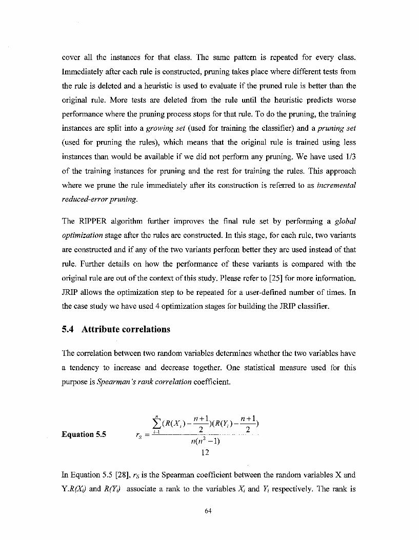
cover all the instances for that class. The same pattern is repeated for every class.
Immediately after each rule is constructed, pruning takes place where different tests from
the rule is deleted and a heuristic is used to evaluate if the pruned rule is better than the
original rule. More tests are deleted from the rule until the heuristic predicts worse
performance where the pruning process stops for that rule. To do the pruning, the training
instances are split into a growing set (used for training the classifier) and a pruning set
(used for pruning the rules), which means that the original rule is trained using less
instances than would be available if we did not perform any pruning. We have used 1/3
of the training instances for pruning and the rest for training the rules. This approach
where we prune the rule immediately after its construction is referred to as incremental
reduced-error pruning.
The RIPPER algorithm further improves the final rule set by performing a global
optimization stage after the rules are constructed. In this stage, for each rule, two variants
are constructed and if any of the two variants perform better they are used instead of that
rule. Further details on how the performance of these variants is compared with the
original rule are out of the context of this study. Please refer to [25] for more information.
JRIP allows the optimization step to be repeated for a user-defined number of times. In
the case study we have used 4 optimization stages for building the JRIP classifier.
5.4 Attribute correlations
The correlation between two random variables determines whether the two variables have
a tendency to increase and decrease together. One statistical measure used for this
purpose is Spearman's rank correlation coefficient.
£(*(*, )-^x*tf)-^±I) Equation 5.5 rs = —
n(n -1) 12
In Equation 5.5 [28], rs is the Spearman coefficient between the random variables X and
Y.R(Xj) and R(Yt) associate a rank to the variables Xt and Yt respectively. The rank is
64
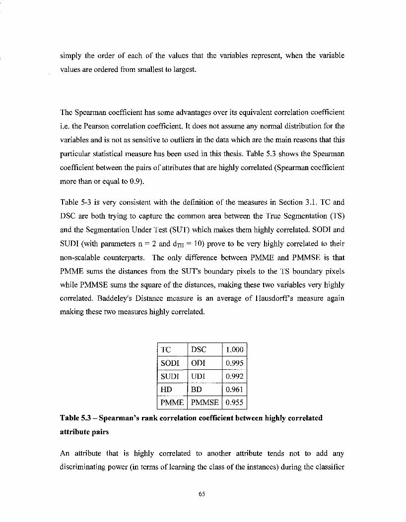
simply the order of each of the values that the variables represent, when the variable
values are ordered from smallest to largest.
The Spearman coefficient has some advantages over its equivalent correlation coefficient
i.e. the Pearson correlation coefficient. It does not assume any normal distribution for the
variables and is not as sensitive to outliers in the data which are the main reasons that this
particular statistical measure has been used in this thesis. Table 5.3 shows the Spearman
coefficient between the pairs of attributes that are highly correlated (Spearman coefficient
more than or equal to 0.9).
Table 5-3 is very consistent with the definition of the measures in Section 3.1. TC and
DSC are both trying to capture the common area between the True Segmentation (TS)
and the Segmentation Under Test (SUT) which makes them highly correlated. SODI and
SUDI (with parameters n = 2 and dra = 10) prove to be very highly correlated to their
non-scalable counterparts. The only difference between PMME and PMMSE is that
PMME sums the distances from the SUT's boundary pixels to the TS boundary pixels
while PMMSE sums the square of the distances, making these two variables very highly
correlated. Baddeley's Distance measure is an average of Hausdorff s measure again
making these two measures highly correlated.
TC
SODI
SUDI
HD
PMME
DSC
ODI
UDI
BD
PMMSE
1.000
0.995
0.992
0.961
0.955
Table 5.3 - Spearman's rank correlation coefficient between highly correlated
attribute pairs
An attribute that is highly correlated to another attribute tends not to add any
discriminating power (in terms of learning the class of the instances) during the classifier
65

learning process. In the case where many correlated attributes exist it may be better to
remove some of them to reduce the classifier construction time. In our case as the number
of the attributes is still not a significant number we let the classifier decide which
attributes to choose and also attempt to filter the attributes using filters and wrappers
(Section 5.5).
5.5 Attribute sets
To compare the performance of the different classifiers, 9 different attribute sets have
been considered (Table 5.4) to teach the machine learning algorithms.
1
2
3
4
5
6
7
8
9
Attribute Set
TC-DSC-TPVF-FPVF-AVD-ANVD
TC-DSC-AVD-ANVD
TC-FPVF
BD-HD-PFOM-RMSSD-ADBD-SODI-ODI-SUDI-UDI-PAD-PMME-PMMSE
HD-BD-PFOM-RMSSD-ODI-UDI-PAD
PFOM-SODI-SUDI
TC-DSC-TPVF-FPVF-AVD-ANVD-BD-HD-PFOM-RMSSD-ADBD-SODI-ODI-SUDI-UDI-PAD-PMME-PMMSE
TC-DSC-AVD-ANVD-HD-RMSSD-ODI-UDI
TC-FPVF-SODI
Selection Criteria
Overlap and volume difference measures
Overlap and volume difference measures chosen by the CFS filter using exhaustive search
Overlap and volume difference measures chosen by the J48 decision tree wrapper using forward selection greedy search
Geometrical measures
Geometrical measures chosen by the CFS filter using exhaustive search
Geometrical measures chosen by the J48 decision tree wrapper using forward selection greedy search
All measures
All measures chosen by the CFS filter using exhaustive search
All measures chosen by the J48 decision tree wrapper using forward selection greedy search
OV
OVC
OVW
G
GC
GW
A
AC
AW
Table 5.4 - Attribute sets and their selection criteria
Three categories of measures have been chosen as the base attribute sets for training the
classifiers: overlap and volume difference, geometrical and all the measures. We want to
see how well the different types of comparison measures would do standalone and what
66
would be the effect of combining these measures. The overlap and volume difference
measures have been combined together. These measures convey less information
regarding the differences between the two segmentations (specifically do not consider the
shape differences) and have less complexity in terms of implementation compared to the
geometrical measures. We may refer to these measures as simple measures.
In order to investigate how the classifier performance would change when built using a
filtered set of attributes we have applied the Correlation-based Feature Selection (CFS)
filter and a J48 based wrapper to the three main categories of attribute sets creating 6
more attribute sets.
Filters and wrappers attempt at taking out attributes that do not add any significant
improvement in building a better classifier; also taking into consideration the association
between the instance attributes and the instance class in their decision making {supervised
attribute selection methods). The main motivation for choosing a wrapper and CFS filter
were the benchmarking results of different attribute selection methods in reference [26].
Correlation-based Feature Selection (CFS) chooses a subset of attributes from the
original attribute set that have a high correlation with the class and a low correlation with
each other. Wrappers select attributes by first training a classifier from different subsets
of the original attribute set and choosing the subset of attributes that trains the best
performing classifier.
Filters and wrappers all require searching the subset space applying their evaluation
criteria to each subset and choosing the best one. Choosing an exhaustive search method
may seem to be the best option at all times but as the number of attributes goes up the
search time for all the subsets also increases. Considering that the evaluation criteria have
to also be applied to all the found subsets using an exhaustive search method may seem
prohibitive. This specially comes into picture when choosing a wrapper method where a
classifier has to be built for every subset found. For this reason, greedy search methods
such as forward or backward hill climbing search are used to search the attribute space
for subsets. In a forward hill climbing search method, we start from an empty subset and
check the evaluation criteria to find the best single attribute. In the next stage, we add
67
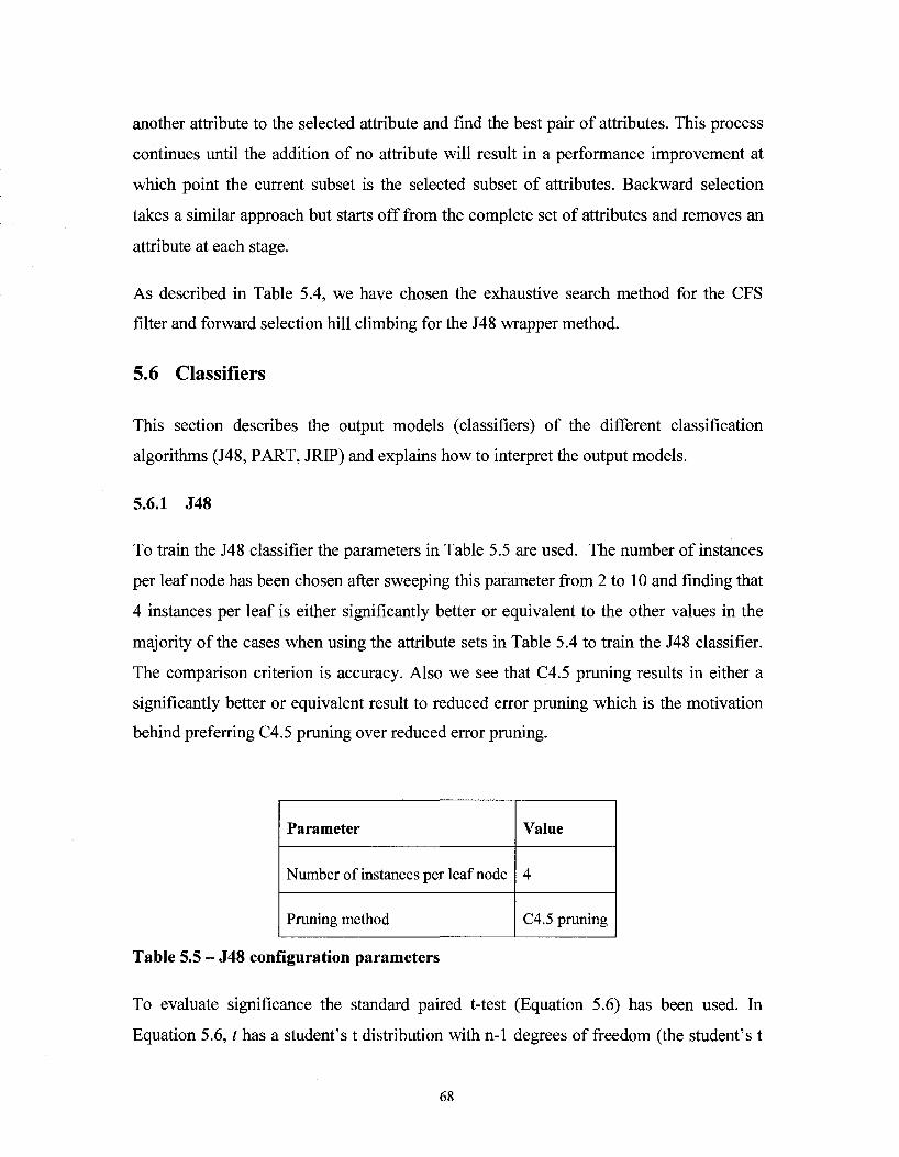
another attribute to the selected attribute and find the best pair of attributes. This process
continues until the addition of no attribute will result in a performance improvement at
which point the current subset is the selected subset of attributes. Backward selection
takes a similar approach but starts off from the complete set of attributes and removes an
attribute at each stage.
As described in Table 5.4, we have chosen the exhaustive search method for the CFS
filter and forward selection hill climbing for the J48 wrapper method.
5.6 Classifiers
This section describes the output models (classifiers) of the different classification
algorithms (J48, PART, JRIP) and explains how to interpret the output models.
5.6.1 J48
To train the J48 classifier the parameters in Table 5.5 are used. The number of instances
per leaf node has been chosen after sweeping this parameter from 2 to 10 and finding that
4 instances per leaf is either significantly better or equivalent to the other values in the
majority of the cases when using the attribute sets in Table 5.4 to train the J48 classifier.
The comparison criterion is accuracy. Also we see that C4.5 pruning results in either a
significantly better or equivalent result to reduced error pruning which is the motivation
behind preferring C4.5 pruning over reduced error pruning.
Parameter
Number of instances per leaf node
Pruning method
Value
4
C4.5 pruning
Table 5.5 - J48 configuration parameters
To evaluate significance the standard paired t-test (Equation 5.6) has been used. In
Equation 5.6, t has a student's t distribution with n-1 degrees of freedom (the student's t
68
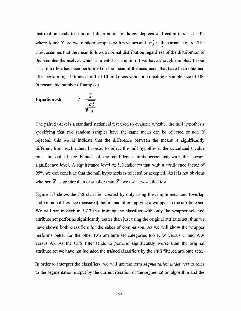
distribution tends to a normal distribution for larger degrees of freedom), d = X - Y,
where X and Y are two random samples with n values and cr] is the variance of d . The
t-test assumes that the mean follows a normal distribution regardless of the distribution of
the samples themselves which is a valid assumption if we have enough samples. In our
case, the t-test has been performed on the mean of the accuracies that have been obtained
after performing 10 times stratified 10 fold cross validation creating a sample size of 100
(a reasonable number of samples).
Equation 5.6 t =
The paired t-test is a standard statistical test used to evaluate whether the null hypothesis
specifying that two random samples have the same mean can be rejected or not. If
rejected, this would indicate that the difference between the means is significantly
different from each other. In order to reject the null hypothesis, the calculated t value
must lie out of the bounds of the confidence limits associated with the chosen
significance level. A significance level of 5% indicates that with a confidence factor of
95% we can conclude that the null hypothesis is rejected or accepted. As it is not obvious
whether X is greater than or smaller than Y, we use a two-tailed test.
Figure 5.7 shows the J48 classifier created by only using the simple measures (overlap
and volume difference measures), before and after applying a wrapper to the attribute set.
We will see in Section 5.7.3 that training the classifier with only the wrapper selected
attribute set performs significantly better than just using the original attribute set, thus we
have shown both classifiers for the sakes of comparison. As we will show the wrapper
performs better for the other two attribute set categories too (GW versus G and AW
versus A). As the CFS filter tends to perform significantly worse than the original
attribute set we have not included the trained classifiers by the CFS filtered attribute sets.
In order to interpret the classifiers, we will use the term segmentation under test to refer
to the segmentation output by the current iteration of the segmentation algorithm and the
<7,
69
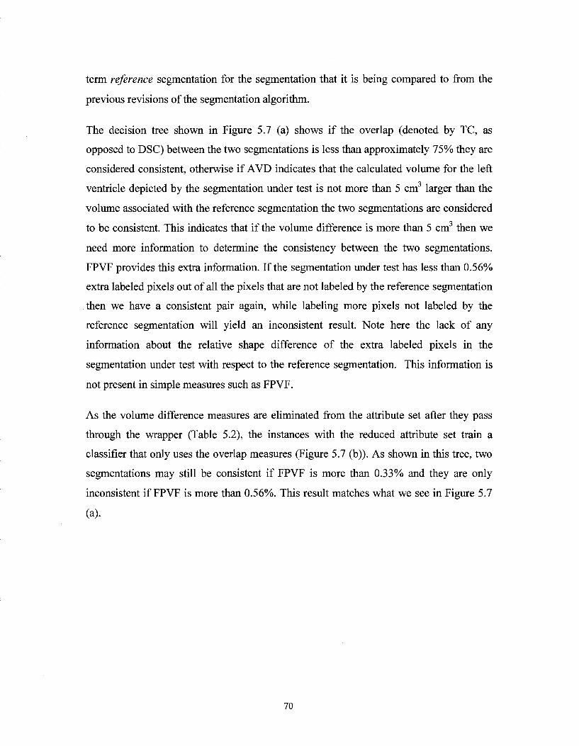
term reference segmentation for the segmentation that it is being compared to from the
previous revisions of the segmentation algorithm.
The decision tree shown in Figure 5.7 (a) shows if the overlap (denoted by TC, as
opposed to DSC) between the two segmentations is less than approximately 75% they are
considered consistent, otherwise if AVD indicates that the calculated volume for the left
ventricle depicted by the segmentation under test is not more than 5 cm3 larger than the
volume associated with the reference segmentation the two segmentations are considered
to be consistent. This indicates that if the volume difference is more than 5 cm then we
need more information to determine the consistency between the two segmentations.
FPVF provides this extra information. If the segmentation under test has less than 0.56%
extra labeled pixels out of all the pixels that are not labeled by the reference segmentation
then we have a consistent pair again, while labeling more pixels not labeled by the
reference segmentation will yield an inconsistent result. Note here the lack of any
information about the relative shape difference of the extra labeled pixels in the
segmentation under test with respect to the reference segmentation. This information is
not present in simple measures such as FPVF.
As the volume difference measures are eliminated from the attribute set after they pass
through the wrapper (Table 5.2), the instances with the reduced attribute set train a
classifier that only uses the overlap measures (Figure 5.7 (b)). As shown in this tree, two
segmentations may still be consistent if FPVF is more than 0.33% and they are only
inconsistent if FPVF is more than 0.56%. This result matches what we see in Figure 5.7
(a).
70
;sifier Free Visualize r: 1 'y: -i 9:1U -trees. Tre<=. VIHW
<= 0.7525 > 0.7525
=•5.
<= 0.005575 > 0.005575
, Weka Classifier Tree Visualizer: 21:28:00 - trees.J40 (overla... ' - ' n l^j j i
'•Tree View "—~"
<= 0 7525 > 0.7525
FPVF
<= 0.00331 8 > 0.00331 8
••F8VF
«= 0.005575 > 0.005575
Figure 5.7 - (a) Top: J48 classifier trained with simple measures (OV) (b) Bottom:
J48 classifier trained with the simple measures selected using J48 wrapper (OVW)
71
The numbers in the parentheses respectively (from left to right) represent the number of
training instances that reach that leaf node and the number of these instances that are in
correctly classified by that leaf node. The incorrect classifications are a result of pruning;
otherwise we would have a very over-fitted tree to the training data that would not
perform well on unknown instances. Paths that reach leaf nodes with less misclassified
instances are more reliable paths i.e. we have more confidence in the prediction of the
decision tree if our unknown instance is classified by the leaf node in these paths. Also
note that a leaf cannot be created with less than 4 instances in that leaf as per our
configuration parameters (Table 5.5).
Figure 5.8 shows the classifiers trained by geometrical measures, before and after
applying a wrapper. Baddeley's distance has been preferred to its more noise-sensitive
counterpart, Hausdorff s distance and is the main discriminating factor for classifying the
negative instances, determining that 66% (51 out of 77) of the negative instances
(inconsistent pairs) have a Baddeley distance of more than 16.73. We also see 92 out of
the 104 positive instances (consistent pairs) do not exceed a Baddeley distance of 16.73
and an ODI distance of 2.10 i.e. 88% of the consistent pairs in the training dataset. We
observe in this classifier that the split made by UDI is somewhat confusing as you would
usually expect more inconsistency when UDI has a larger value as opposed to a smaller
one. This split just means that we have 4 inconsistent pairs in the training set with a UDI
of less than 1.67 and 6 consistent pairs with a UDI of more than 1.67. This may indicate
that using UDI by itself may not be a good indicator of the consistency between two
segmentations, also confirming that using many measures in conjunction with each other
is more effective in classifying consistent or inconsistent pairs rather than only using one
measure to predict consistency. For example, if our training set is biased towards
segmentations with a lot of oversegmentation, then UDI will not be a good performer as
it only considers the distance of the undersegmented pixels to the reference boundary.
These kind of attribute splits will be much more unlikely upon availability of larger
training sets with more representative instances for each class.
72
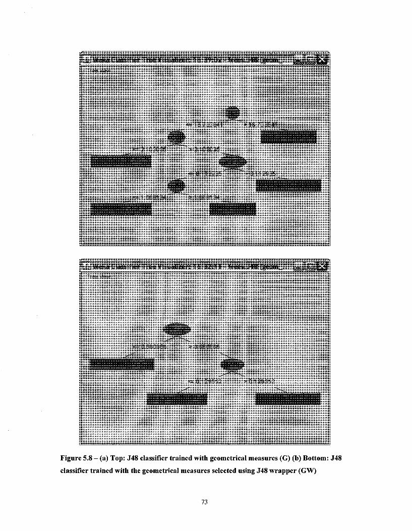
Tlee =
BO
==16.733841 > 16.733841
<= 2.103035 > 2.103035
TUQI
<= 0.112935 > 0.112935
<= 1.668134 > 1.668134
Weka Classifier Tree Visualizer: 16:32:11 - trees.J48 (geom_... ; . I 'D j^Sj
iHiii^H
PFOM
*= 0.680966 > 0.680966
SGDt
<= 0.1 29552 * 0.129552
Figure 5.8 - (a) Top: J48 classifier trained with geometrical measures (G) (b) Bottom: J48
classifier trained with the geometrical measures selected using J48 wrapper (GW)
73
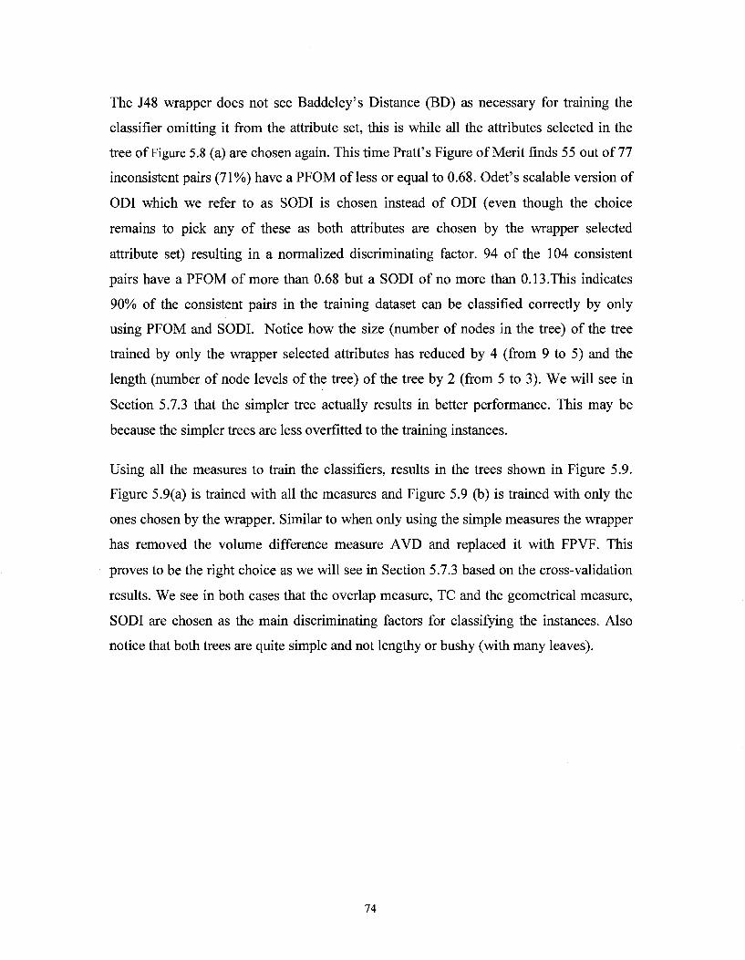
The J48 wrapper does not see Baddeley's Distance (BD) as necessary for training the
classifier omitting it from the attribute set, this is while all the attributes selected in the
tree of Figure 5.8 (a) are chosen again. This time Pratt's Figure of Merit finds 55 out of 77
inconsistent pairs (71%) have a PFOM of less or equal to 0.68. Odet's scalable version of
ODI which we refer to as SODI is chosen instead of ODI (even though the choice
remains to pick any of these as both attributes are chosen by the wrapper selected
attribute set) resulting in a normalized discriminating factor. 94 of the 104 consistent
pairs have a PFOM of more than 0.68 but a SODI of no more than 0.13.This indicates
90% of the consistent pairs in the training dataset can be classified correctly by only
using PFOM and SODI. Notice how the size (number of nodes in the tree) of the tree
trained by only the wrapper selected attributes has reduced by 4 (from 9 to 5) and the
length (number of node levels of the tree) of the tree by 2 (from 5 to 3). We will see in
Section 5.7.3 that the simpler tree actually results in better performance. This may be
because the simpler trees are less overfitted to the training instances.
Using all the measures to train the classifiers, results in the trees shown in Figure 5.9.
Figure 5.9(a) is trained with all the measures and Figure 5.9 (b) is trained with only the
ones chosen by the wrapper. Similar to when only using the simple measures the wrapper
has removed the volume difference measure AVD and replaced it with FPVF. This
proves to be the right choice as we will see in Section 5.7.3 based on the cross-validation
results. We see in both cases that the overlap measure, TC and the geometrical measure,
SODI are chosen as the main discriminating factors for classifying the instances. Also
notice that both trees are quite simple and not lengthy or bushy (with many leaves).
74
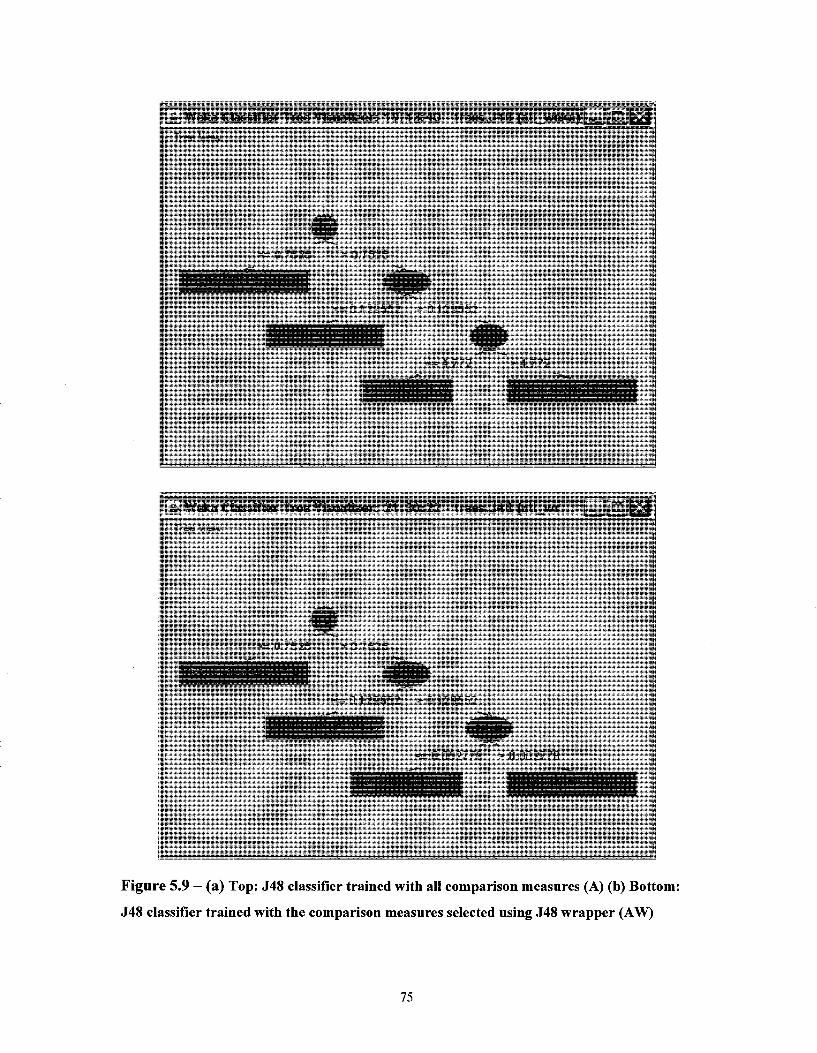
Wekd Classifier Treu Visutjliiur: 19:4 3M0 trues..148 (till..
•iltfHHi
TC.
<= 0.7525 > 0.7525
;|)¥vbfelst^i'^8'.0^.d)j i'SOOt
<= 0.1 29552 5=0.129552
*MD
<= 4.772 4.772
Wekd Ctassiliur Irnu Visiwli^er: 71:30:; (all_wr... . - . J O ; ^
Tree View •
TC
<= 0.7525 > 0 7525
•iSOW
<= 0.129552 > 0 129552
«= 0.002778 > 0 002778
Figure 5.9 — (a) Top: J48 classifier trained with all comparison measures (A) (b) Bottom:
J48 classifier trained with the comparison measures selected using J48 wrapper (AW)
75
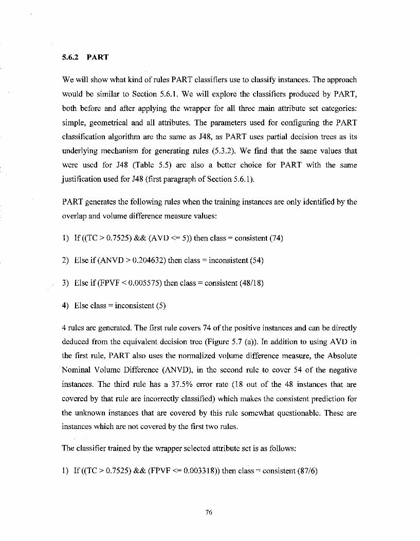
5.6.2 PART
We will show what kind of rules PART classifiers use to classify instances. The approach
would be similar to Section 5.6.1. We will explore the classifiers produced by PART,
both before and after applying the wrapper for all three main attribute set categories:
simple, geometrical and all attributes. The parameters used for configuring the PART
classification algorithm are the same as J48, as PART uses partial decision trees as its
underlying mechanism for generating rules (5.3.2). We find that the same values that
were used for J48 (Table 5.5) are also a better choice for PART with the same
justification used for J48 (first paragraph of Section 5.6.1).
PART generates the following rules when the training instances are only identified by the
overlap and volume difference measure values:
1) If ((TC > 0.7525) && (AVD <= 5)) then class = consistent (74)
2) Else if (ANVD > 0.204632) then class = inconsistent (54)
3) Else if (FPVF < 0.005575) then class = consistent (48/18)
4) Else class = inconsistent (5)
4 rules are generated. The first rule covers 74 of the positive instances and can be directly
deduced from the equivalent decision tree (Figure 5.7 (a)). In addition to using AVD in
the first rule, PART also uses the normalized volume difference measure, the Absolute
Nominal Volume Difference (ANVD), in the second rule to cover 54 of the negative
instances. The third rule has a 37.5% error rate (18 out of the 48 instances that are
covered by that rule are incorrectly classified) which makes the consistent prediction for
the unknown instances that are covered by this rule somewhat questionable. These are
instances which are not covered by the first two rules.
The classifier trained by the wrapper selected attribute set is as follows:
1) If ((TC > 0.7525) && (FPVF <= 0.003318)) then class = consistent (87/6)
76
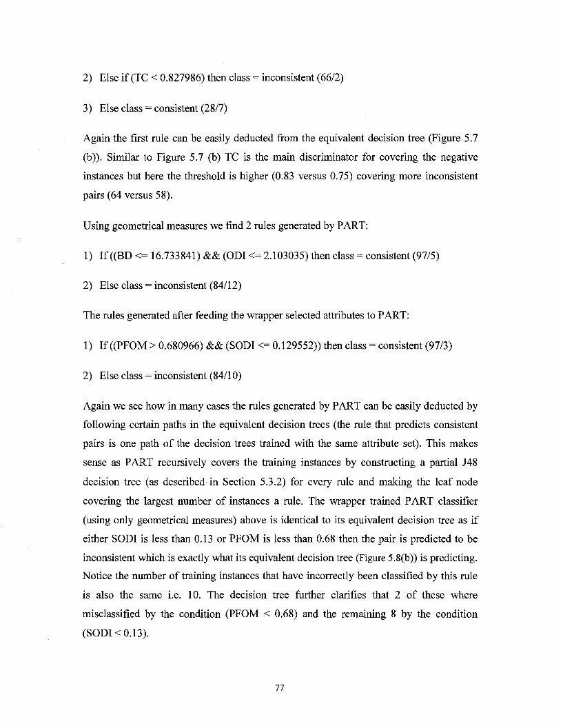
2) Else if (TC < 0.827986) then class = inconsistent (66/2)
3) Else class = consistent (28/7)
Again the first rule can be easily deducted from the equivalent decision tree (Figure 5.7
(b)). Similar to Figure 5.7 (b) TC is the main discriminator for covering the negative
instances but here the threshold is higher (0.83 versus 0.75) covering more inconsistent
pairs (64 versus 58).
Using geometrical measures we find 2 rules generated by PART:
1) If ((BD <= 16.733841) && (ODI <= 2.103035) then class = consistent (97/5)
2) Else class = inconsistent (84/12)
The rules generated after feeding the wrapper selected attributes to PART:
1) If ((PFOM > 0.680966) && (SODI <= 0.129552)) then class - consistent (97/3)
2) Else class = inconsistent (84/10)
Again we see how in many cases the rules generated by PART can be easily deducted by
following certain paths in the equivalent decision trees (the rule that predicts consistent
pairs is one path of the decision trees trained with the same attribute set). This makes
sense as PART recursively covers the training instances by constructing a partial J48
decision tree (as described in Section 5.3.2) for every rule and making the leaf node
covering the largest number of instances a rule. The wrapper trained PART classifier
(using only geometrical measures) above is identical to its equivalent decision tree as if
either SODI is less than 0.13 or PFOM is less than 0.68 then the pair is predicted to be
inconsistent which is exactly what its equivalent decision tree (Figure 5.8(b)) is predicting.
Notice the number of training instances that have incorrectly been classified by this rule
is also the same i.e. 10. The decision tree further clarifies that 2 of these where
misclassified by the condition (PFOM < 0.68) and the remaining 8 by the condition
(SODK0.13).
77
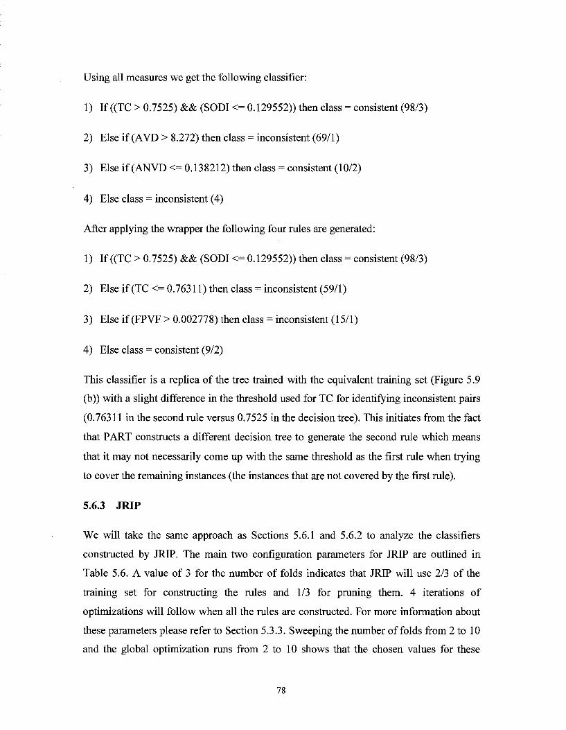
Using all measures we get the following classifier:
1) If ((TC > 0.7525) && (SODI <= 0.129552)) then class = consistent (98/3)
2) Else if (AVD > 8.272) then class = inconsistent (69/1)
3) Else if (ANVD <= 0.138212) then class = consistent (10/2)
4) Else class = inconsistent (4)
After applying the wrapper the following four rules are generated:
1) If ((TC > 0.7525) && (SODI <= 0.129552)) then class = consistent (98/3)
2) Else if (TC <= 0.76311) then class = inconsistent (59/1)
3) Else if (FPVF > 0.002778) then class = inconsistent (15/1)
4) Else class = consistent (9/2)
This classifier is a replica of the tree trained with the equivalent training set (Figure 5.9
(b)) with a slight difference in the threshold used for TC for identifying inconsistent pairs
(0.76311 in the second rule versus 0.7525 in the decision tree). This initiates from the fact
that PART constructs a different decision tree to generate the second rule which means
that it may not necessarily come up with the same threshold as the first rule when trying
to cover the remaining instances (the instances that are not covered by the first rule).
5.6.3 JRIP
We will take the same approach as Sections 5.6.1 and 5.6.2 to analyze the classifiers
constructed by JRIP. The main two configuration parameters for JRIP are outlined in
Table 5.6. A value of 3 for the number of folds indicates that JRIP will use 2/3 of the
training set for constructing the rules and 1/3 for pruning them. 4 iterations of
optimizations will follow when all the rules are constructed. For more information about
these parameters please refer to Section 5.3.3. Sweeping the number of folds from 2 to 10
and the global optimization runs from 2 to 10 shows that the chosen values for these
78
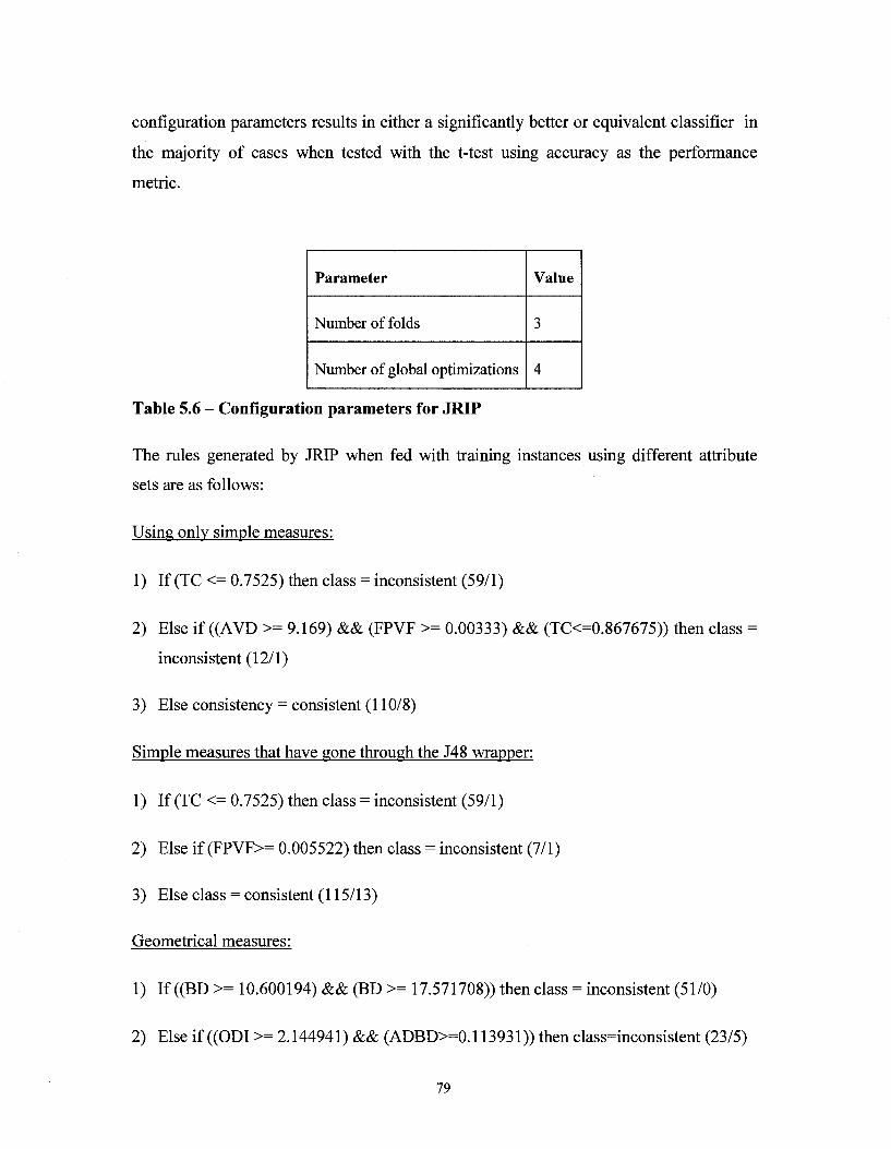
configuration parameters results in either a significantly better or equivalent classifier in
the majority of cases when tested with the t-test using accuracy as the performance
metric.
Parameter
Number of folds
Number of global optimizations
Value
3
4
Table 5.6 - Configuration parameters for JRIP
The rules generated by JRIP when fed with training instances using different attribute
sets are as follows:
Using only simple measures:
1) If (TC <= 0.7525) then class = inconsistent (59/1)
2) Else if ((AVD >= 9.169) && (FPVF >= 0.00333) && (TC<=0.867675)) then class =
inconsistent (12/1)
3) Else consistency = consistent (110/8)
Simple measures that have gone through the J48 wrapper:
1) If (TC <= 0.7525) then class = inconsistent (59/1)
2) Else if (FPVF>= 0.005522) then class = inconsistent (7/1)
3) Else class = consistent (115/13)
Geometrical measures:
1) If ((BD >= 10.600194) && (BD >= 17.571708)) then class = inconsistent (51/0)
2) Else if ((ODI >= 2.144941) && (ADBD>=0.113931)) then class=inconsistent (23/5)
79
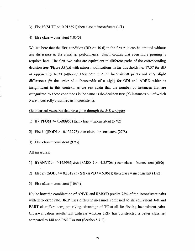
3) Else if (SUDI <= 0.016691) then class = inconsistent (4/1)
4) Else class = consistent (103/5)
We see here that the first condition (BD >= 10.6) in the first rule can be omitted without
any difference in the classifier performance. This indicates that even more pruning is
required here. The first two rules are equivalent to different paths of the corresponding
decision tree (Figure 5.8(a)) with minor modifications in the thresholds i.e. 17.57 for BD
as opposed to 16.73 (although they both find 51 inconsistent pairs) and very slight
differences (in the order of a thousandth of a digit) for ODI and ADBD which is
insignificant in this context, as we see again that the number of instances that are
categorized by these conditions is the same as the decision tree (23 instances out of which
5 are incorrectly classified as inconsistent).
Geometrical measures that have gone through the J48 wrapper:
1) If ((PFOM <= 0.680966) then class - inconsistent (57/2)
2) Else if ((SODI >= 0.131275) then class = inconsistent (27/8)
3) Else class = consistent (97/3)
All measures:
1) If (ANVD >= 0.148995) && (RMSSD >= 4.357064) then class = inconsistent (60/0)
2) Else if ((SODI >= 0.131275) && (AVD >= 5.061)) then class = inconsistent (15/2)
3) Else class = consistent (106/4)
Notice how the combination of ANVD and RMSSD predict 78% of the inconsistent pairs
with zero error rate. JRIP uses different measures compared to its equivalent J48 and
PART classifiers here, not taking advantage of TC at all for finding inconsistent pairs.
Cross-validation results will indicate whether JRIP has constructed a better classifier
compared to J48 and PART or not (Section 5.7.2).
80
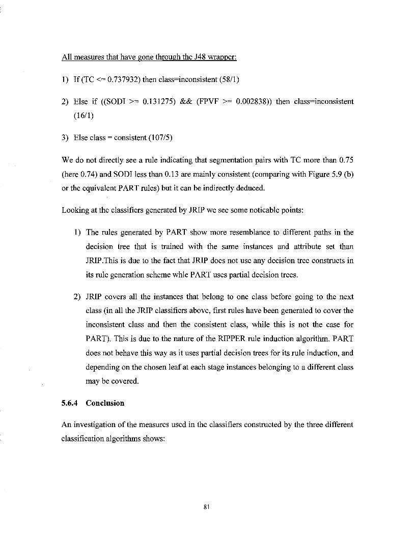
All measures that have gone through the J48 wrapper:
1) If (TC <= 0.737932) then class=inconsistent (58/1)
2) Else if ((SODI > - 0.131275) && (FPVF >= 0.002838)) then class=inconsistent
(16/1)
3) Else class = consistent (107/5)
We do not directly see a rule indicating that segmentation pairs with TC more than 0.75
(here 0.74) and SODI less than 0.13 are mainly consistent (comparing with Figure 5.9 (b)
or the equivalent PART rules) but it can be indirectly deduced.
Looking at the classifiers generated by JRIP we see some noticable points:
1) The rules generated by PART show more resemblance to different paths in the
decision tree that is trained with the same instances and attribute set than
JRIP.This is due to the fact that JRIP does not use any decision tree constructs in
its rule generation scheme whle PART uses partial decision trees.
2) JRIP covers all the instances that belong to one class before going to the next
class (in all the JRIP classifiers above, first rules have been generated to cover the
inconsistent class and then the consistent class, while this is not the case for
PART). This is due to the nature of the RIPPER rule induction algorithm. PART
does not behave this way as it uses partial decision trees for its rule induction, and
depending on the chosen leaf at each stage instances belonging to a different class
may be covered.
5.6.4 Conclusion
An investigation of the measures used in the classifiers constructed by the three different
classification algorithms shows:
81
1) TC and FPVF are the most popular overlap measures. TC was preferred to
DSC which is very highly correlated to it (Table 5.3). Also TPVF was never
chosen.
2) SODI is the most popular geometrical measure being used in close to all the
classifiers that have geometrical measures involved in training them.
3) Good discriminators for negative instances (inconsistent pairs) are:
a. Using only simple measures: TC
b. Using only geometrical measures: BD, PFOM
c. Using all measures: TC and the combination of ANVD and RMSSD as
discovered by JRIP.
78% (using only simple measures) to 91% (using all measures) of the negative
instances are covered with the above measures.
4) Good discriminators for positive instances (consistent pairs) are the following
combinations:
a. Using only simple measures: TC and AVD or TC and FPVF.
b. Using only geometrical measures: BD and ODI or PFOM and SODI.
c. Using all measures: TC and SODI.
Around 75% of the positive instances are covered by the above combinations.
5) When using all the measures, TC was the main discriminator for negative
instances and the combination of TC and SODI was the main discriminator for
the positive instances. If TC determines that the two segmentations have a less
than 75% overlap, then the two segmentations are inconsistent. Otherwise if
SODI determines that the average oversegmented pixels have a normalized
distance of less than 0.13 to the boundary of the reference segmentation then
82
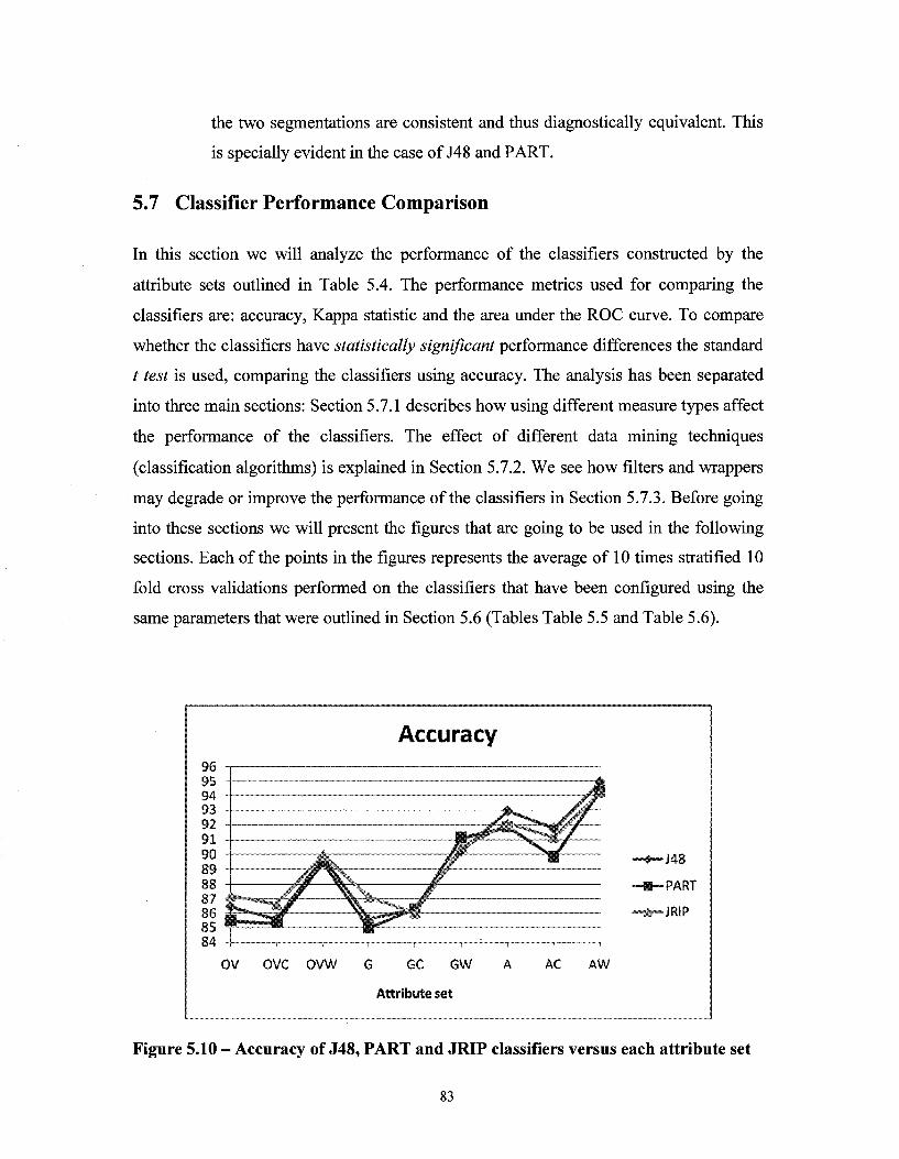
the two segmentations are consistent and thus diagnostically equivalent. This
is specially evident in the case of J48 and PART.
5.7 Classifier Performance Comparison
In this section we will analyze the performance of the classifiers constructed by the
attribute sets outlined in Table 5.4. The performance metrics used for comparing the
classifiers are: accuracy, Kappa statistic and the area under the ROC curve. To compare
whether the classifiers have statistically significant performance differences the standard
t test is used, comparing the classifiers using accuracy. The analysis has been separated
into three main sections: Section 5.7.1 describes how using different measure types affect
the performance of the classifiers. The effect of different data mining techniques
(classification algorithms) is explained in Section 5.7.2. We see how filters and wrappers
may degrade or improve the performance of the classifiers in Section 5.7.3. Before going
into these sections we will present the figures that are going to be used in the following
sections. Each of the points in the figures represents the average of 10 times stratified 10
fold cross validations performed on the classifiers that have been configured using the
same parameters that were outlined in Section 5.6 (Tables Table 5.5 and Table 5.6).
Accuracy
J48
PART
JR!P
ov ovc ovw GC GW
Attribute set
AC AW
Figure 5.10 - Accuracy of J48, PART and JRIP classifiers versus each attribute set
83
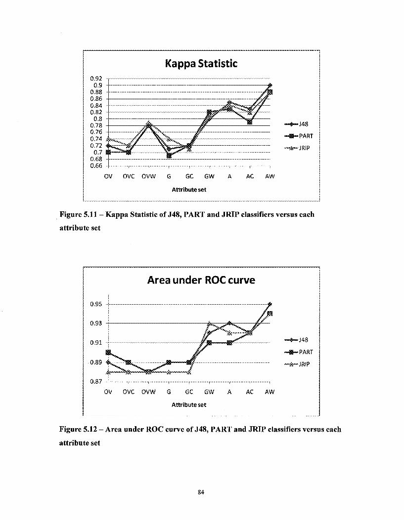
Kappa Statistic 0.92
0.66
OV OVC OVW GC GW
Attribute set
AC AW
J48
PART
JRIP
Figure 5.11 - Kappa Statistic of J48, PART and JRIP classifiers versus each
attribute set
0.87
Area under ROC curve
»J48
•PART
•JRIP
1 1 1 1 1 1—
OV OVC OVW G GC GW A
Attribute set
AC AW
Figure 5.12 - Area under ROC curve of J48, PART and JRIP classifiers versus each
attribute set
84
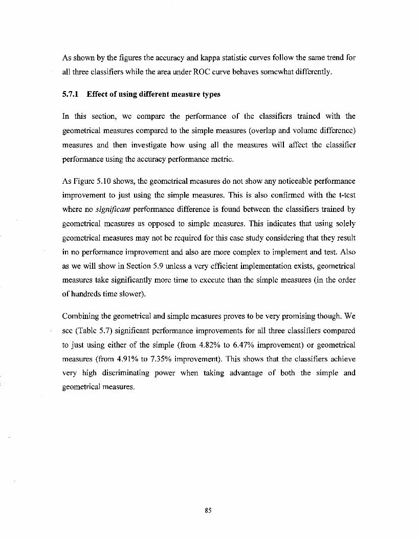
As shown by the figures the accuracy and kappa statistic curves follow the same trend for
all three classifiers while the area under ROC curve behaves somewhat differently.
5.7.1 Effect of using different measure types
In this section, we compare the performance of the classifiers trained with the
geometrical measures compared to the simple measures (overlap and volume difference)
measures and then investigate how using all the measures will affect the classifier
performance using the accuracy performance metric.
As Figure 5.10 shows, the geometrical measures do not show any noticeable performance
improvement to just using the simple measures. This is also confirmed with the t-test
where no significant performance difference is found between the classifiers trained by
geometrical measures as opposed to simple measures. This indicates that using solely
geometrical measures may not be required for this case study considering that they result
in no performance improvement and also are more complex to implement and test. Also
as we will show in Section 5.9 unless a very efficient implementation exists, geometrical
measures take significantly more time to execute than the simple measures (in the order
of hundreds time slower).
Combining the geometrical and simple measures proves to be very promising though. We
see (Table 5.7) significant performance improvements for all three classifiers compared
to just using either of the simple (from 4.82% to 6.47% improvement) or geometrical
measures (from 4.91% to 7.35% improvement). This shows that the classifiers achieve
very high discriminating power when taking advantage of both the simple and
geometrical measures.
85
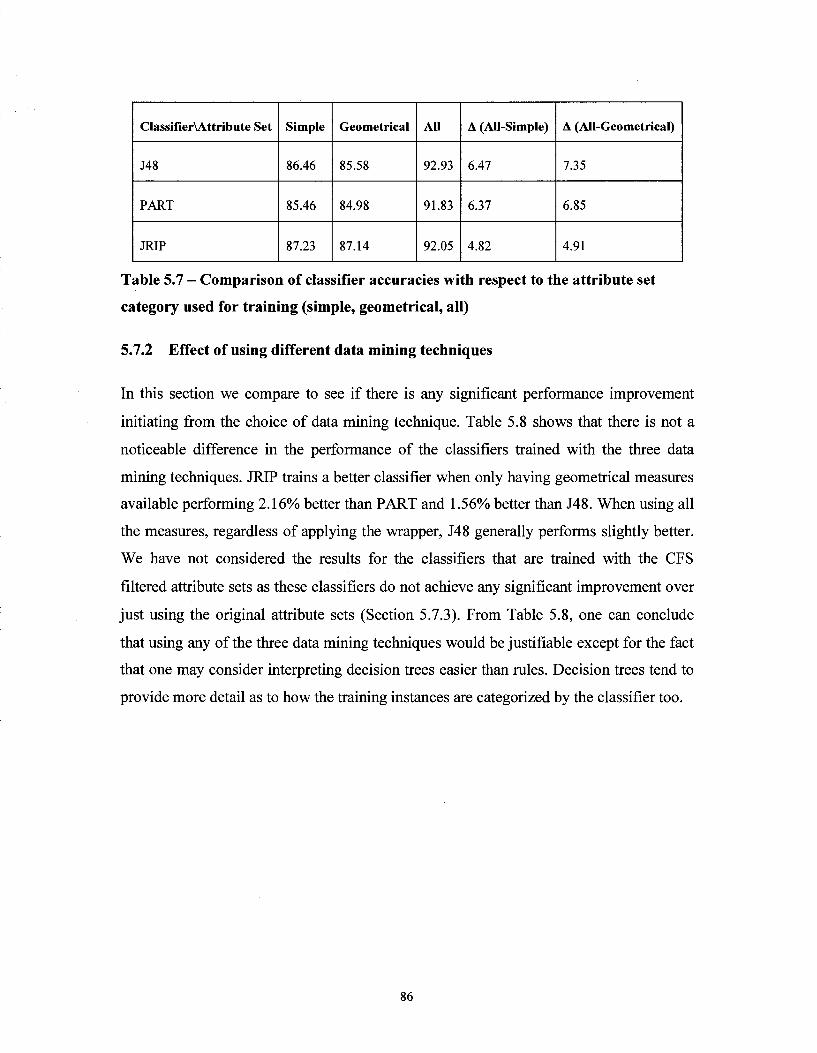
ClassifieiAAttribute Set
J48
PART
JRIP
Simple
86.46
85.46
87.23
Geometrical
85.58
84.98
87.14
All
92.93
91.83
92.05
A (All-Simple)
6.47
6.37
4.82
A (All-Geometrical)
7.35
6.85
4.91
Table 5.7 - Comparison of classifier accuracies with respect to the attribute set
category used for training (simple, geometrical, all)
5.7.2 Effect of using different data mining techniques
In this section we compare to see if there is any significant performance improvement
initiating from the choice of data mining technique. Table 5.8 shows that there is not a
noticeable difference in the performance of the classifiers trained with the three data
mining techniques. JRIP trains a better classifier when only having geometrical measures
available performing 2.16% better than PART and 1.56% better than J48. When using all
the measures, regardless of applying the wrapper, J48 generally performs slightly better.
We have not considered the results for the classifiers that are trained with the CFS
filtered attribute sets as these classifiers do not achieve any significant improvement over
just using the original attribute sets (Section 5.7.3). From Table 5.8, one can conclude
that using any of the three data mining techniques would be justifiable except for the fact
that one may consider interpreting decision trees easier than rules. Decision trees tend to
provide more detail as to how the training instances are categorized by the classifier too.
86
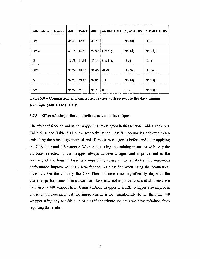
Attribute Set\Classifier
OV
ovw
G
GW
A
AW
J48
86.46
89.78
85.58
90.24
92.93
94.92
PART
85.46
89.50
84.98
91.13
91.83
94.32
JRIP
87.23
90.00
87.14
90.46
92.05
94.21
A(J48-PART)
1
Not Sig.
Not Sig.
-0.89
1.1
0.6
A(J48-JRIP)
Not Sig.
Not Sig.
-1.56
Not Sig.
Not Sig.
0.71
A(PART-JRIP)
-1.77
Not Sig.
-2.16
Not Sig.
Not Sig.
Not Sig.
Table 5.8 - Comparison of classifier accuracies with respect to the data mining
technique (J48, PART, JRIP)
5.7.3 Effect of using different attribute selection techniques
The effect of filtering and using wrappers is investigated in this section. Tables Table 5.9,
Table 5.10 and Table 5.11 show respectively the classifier accuracies achieved when
trained by the simple, geometrical and all measure categories before and after applying
the CFS filter and J48 wrapper. We see that using the training instances with only the
attributes selected by the wrapper always achieve a significant improvement in the
accuracy of the trained classifier compared to using all the attributes; the maximum
performance improvement is 7.16% for the J48 classifier when using the geometrical
measures. On the contrary the CFS filter in some cases significantly degrades the
classifier performance. This shows that filters may not improve results at all times. We
have used a J48 wrapper here. Using a PART wrapper or a JRIP wrapper also improves
classifier performance, but the improvement is not significantly better than the J48
wrapper using any combination of classifier\attribute set, thus we have refrained from
reporting the results.
87
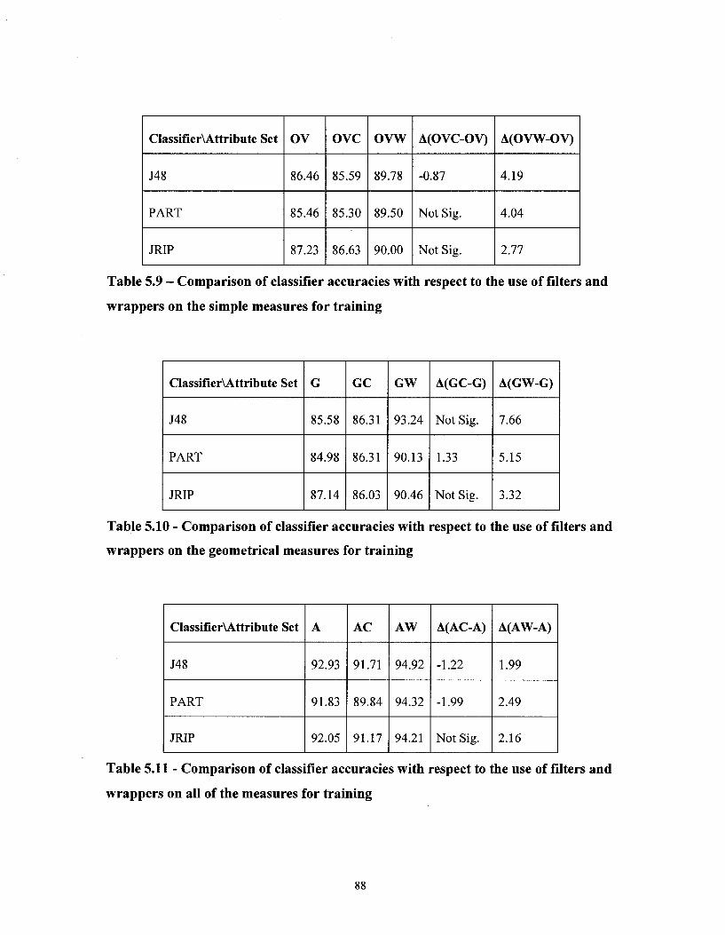
ClassifierYAttribute Set
J48
PART
JRIP
OV
86.46
85.46
87.23
ovc
85.59
85.30
86.63
ovw
89.78
89.50
90.00
A(OVC-OV)
-0.87
Not Sig.
Not Sig.
A(OVW-OV)
4.19
4.04
2.77
Table 5.9 - Comparison of classifier accuracies with respect to the use of filters and
wrappers on the simple measures for training
ClassifierYAttribute Set
J48
PART
JRIP
G
85.58
84.98
87.14
GC
86.31
86.31
86.03
GW
93.24
90.13
90.46
A(GC-G)
Not Sig.
1.33
Not Sig.
A(GW-G)
7.66
5.15
3.32
Table 5.10 - Comparison of classifier accuracies with respect to the use of filters and
wrappers on the geometrical measures for training
ClassifierVAttribute Set
J48
PART
JRIP
A
92.93
91.83
92.05
AC
91.71
89.84
91.17
AW
94.92
94.32
94.21
A(AC-A)
-1.22
-1.99
Not Sig.
A(AW-A)
1.99
2.49
2.16
Table 5.11 - Comparison of classifier accuracies with respect to the use of filters and
wrappers on all of the measures for training
88
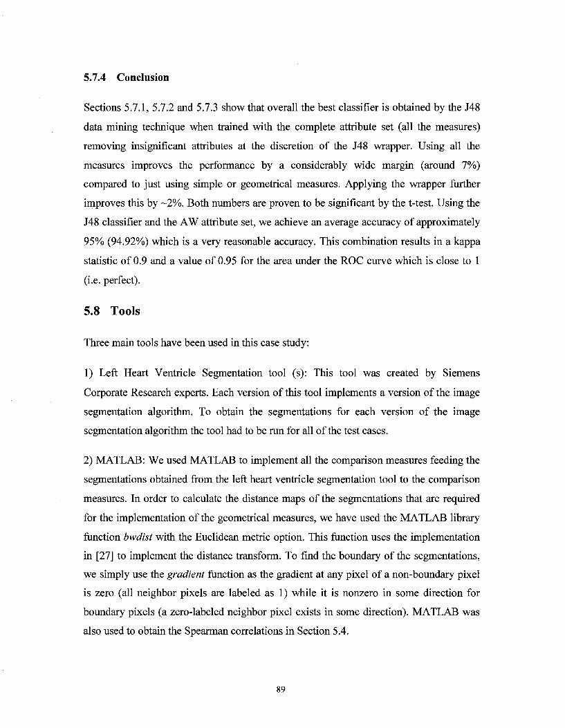
5.7.4 Conclusion
Sections 5.7.1, 5.7.2 and 5.7.3 show that overall the best classifier is obtained by the J48
data mining technique when trained with the complete attribute set (all the measures)
removing insignificant attributes at the discretion of the J48 wrapper. Using all the
measures improves the performance by a considerably wide margin (around 7%)
compared to just using simple or geometrical measures. Applying the wrapper further
improves this by ~2%. Both numbers are proven to be significant by the t-test. Using the
J48 classifier and the AW attribute set, we achieve an average accuracy of approximately
95% (94.92%) which is a very reasonable accuracy. This combination results in a kappa
statistic of 0.9 and a value of 0.95 for the area under the ROC curve which is close to 1
(i.e. perfect).
5.8 Tools
Three main tools have been used in this case study:
1) Left Heart Ventricle Segmentation tool (s): This tool was created by Siemens
Corporate Research experts. Each version of this tool implements a version of the image
segmentation algorithm. To obtain the segmentations for each version of the image
segmentation algorithm the tool had to be run for all of the test cases.
2) MATLAB: We used MATLAB to implement all the comparison measures feeding the
segmentations obtained from the left heart ventricle segmentation tool to the comparison
measures. In order to calculate the distance maps of the segmentations that are required
for the implementation of the geometrical measures, we have used the MATLAB library
function bwdist with the Euclidean metric option. This function uses the implementation
in [27] to implement the distance transform. To find the boundary of the segmentations,
we simply use the gradient function as the gradient at any pixel of a non-boundary pixel
is zero (all neighbor pixels are labeled as 1) while it is nonzero in some direction for
boundary pixels (a zero-labeled neighbor pixel exists in some direction). MATLAB was
also used to obtain the Spearman correlations in Section 5.4.
89
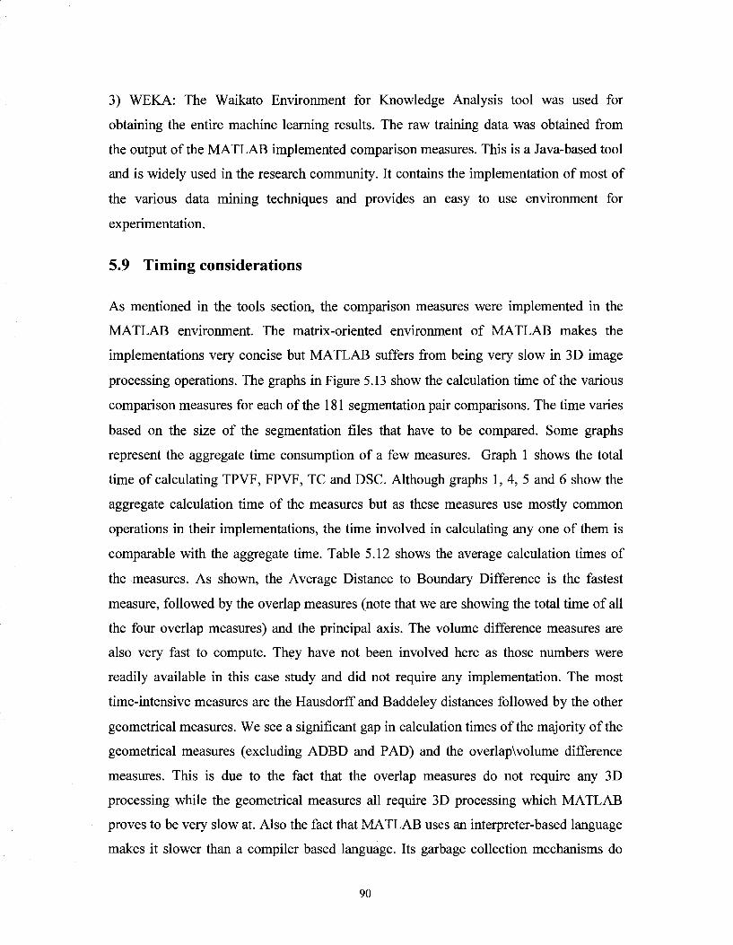
3) WEKA: The Waikato Environment for Knowledge Analysis tool was used for
obtaining the entire machine learning results. The raw training data was obtained from
the output of the MATLAB implemented comparison measures. This is a Java-based tool
and is widely used in the research community. It contains the implementation of most of
the various data mining techniques and provides an easy to use environment for
experimentation.
5.9 Timing considerations
As mentioned in the tools section, the comparison measures were implemented in the
MATLAB environment. The matrix-oriented environment of MATLAB makes the
implementations very concise but MATLAB suffers from being very slow in 3D image
processing operations. The graphs in Figure 5.13 show the calculation time of the various
comparison measures for each of the 181 segmentation pair comparisons. The time varies
based on the size of the segmentation files that have to be compared. Some graphs
represent the aggregate time consumption of a few measures. Graph 1 shows the total
time of calculating TPVF, FPVF, TC and DSC. Although graphs 1, 4, 5 and 6 show the
aggregate calculation time of the measures but as these measures use mostly common
operations in their implementations, the time involved in calculating any one of them is
comparable with the aggregate time. Table 5.12 shows the average calculation times of
the measures. As shown, the Average Distance to Boundary Difference is the fastest
measure, followed by the overlap measures (note that we are showing the total time of all
the four overlap measures) and the principal axis. The volume difference measures are
also very fast to compute. They have not been involved here as those numbers were
readily available in this case study and did not require any implementation. The most
time-intensive measures are the Hausdorff and Baddeley distances followed by the other
geometrical measures. We see a significant gap in calculation times of the majority of the
geometrical measures (excluding ADBD and PAD) and the overlapwolume difference
measures. This is due to the fact that the overlap measures do not require any 3D
processing while the geometrical measures all require 3D processing which MATLAB
proves to be very slow at. Also the fact that MATLAB uses an interpreter-based language
makes it slower than a compiler based language. Its garbage collection mechanisms do
90
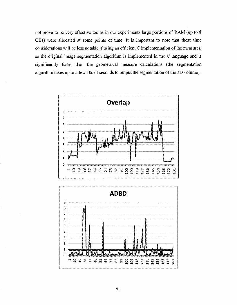
not prove to be very effective too as in our experiments large portions of RAM (up to 8
GBs) were allocated at some points of time. It is important to note that these time
considerations will be less notable if using an efficient C implementation of the measures,
as the original image segmentation algorithm is implemented in the C language and is
significantly faster than the geometrical measure calculations (the segmentation
algorithm takes up to a few 10s of seconds to output the segmentation of the 3D volume).
Overlap
r - j « - ) r - i r - i < H « - ) i c - - i r H l - 4 r - l
ADBD
< H o m o o h ~ > O L n ^ f « f M *-( o «r> oo i>- «3 tn «» m <M «H r - t T H f N p n ^ j ' L n i e r ^ - c o m o o t - H f M m ' ^ w i i o r ^ o o
• < H f - l < H r - l r - i r H < - - ! r - ( r - ( r H
91
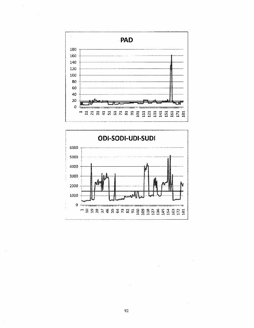
PAD 180
160
140
120
100
80
60
40
ODI-SODI-UDI-SUDI o u u u -
J U U U
3UUU ~
•ynnn _
Iflftrt -
im^"
1 f' i
1*1 1 p
1 f *** l « # JU^ # I , W
r
Tr 1
J 1W Tn ff
_4JJ_. _ L-J
92
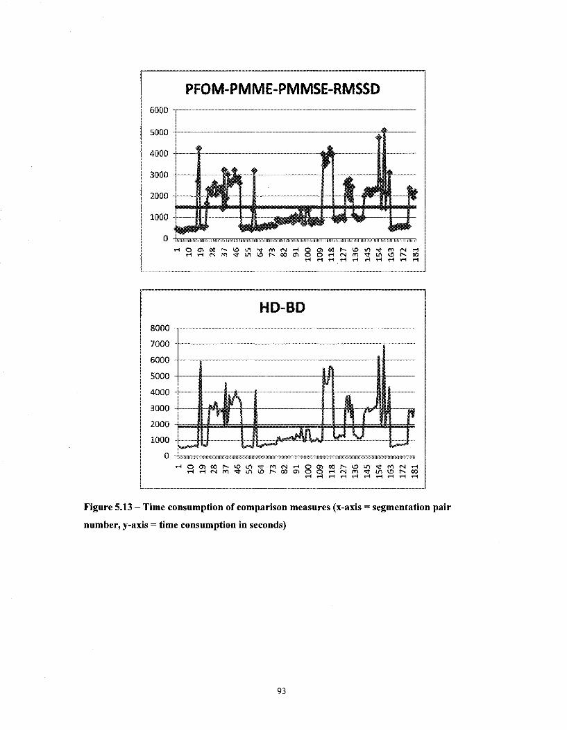
PFOM-PMME-PMMSE-RIViSSD 6000
i H O O > o c ! s « » o w < ! f < i n < M < H O O > o o r , > > u > » r t " i t « n < N ! H * H r t H < H r - t * - « r t t - H i - I H
sooo 7000
6000
5000
4000
3000
2000
1000
0
HD-BD
J jv*#y'^l i %»<i#
H H N f f l ^ W O N 0 0 O l O O H N ( l ) * I A « I M « t H r H i H i - t r - l r H r - l r - t r - l T H
Figure 5.13 - Time consumption of comparison measures (x-axis = segmentation pair
number, y-axis = time consumption in seconds)
93
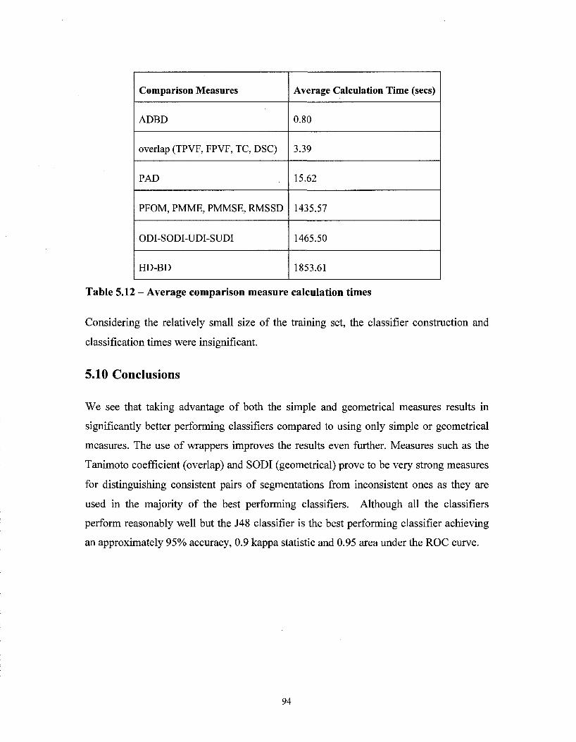
Comparison Measures
ADBD
overlap (TPVF, FPVF, TC, DSC)
PAD
PFOM, PMME, PMMSE, RMSSD
ODI-SODI-UDI-SUDI
HD-BD
Average Calculation Time (sees)
0.80
3.39
15.62
1435.57
1465.50
1853.61
Table 5.12 - Average comparison measure calculation times
Considering the relatively small size of the training set, the classifier construction and
classification times were insignificant.
5.10 Conclusions
We see that taking advantage of both the simple and geometrical measures results in
significantly better performing classifiers compared to using only simple or geometrical
measures. The use of wrappers improves the results even further. Measures such as the
Tanimoto coefficient (overlap) and SODI (geometrical) prove to be very strong measures
for distinguishing consistent pairs of segmentations from inconsistent ones as they are
used in the majority of the best performing classifiers. Although all the classifiers
perform reasonably well but the J48 classifier is the best performing classifier achieving
an approximately 95% accuracy, 0.9 kappa statistic and 0.95 area under the ROC curve.
6 CONCLUSIONS AND FUTURE WORK
The verification procedure for medical image segmentation algorithms is an iterative
process where the same verifications have to be repeated for each version of the image
segmentation algorithm manually until the image segmentation algorithm is evaluated to
be sufficiently correct for the requirements of the application domain. The segmentation
algorithm goes through 10s of revisions until it is finalized. In this thesis, an approach
towards semi-automating this procedure has been proposed. In this approach, the
knowledge gained from the manual evaluation of the first few versions (optimally two) of
the software under test is captured by calculating similarity measures between the pairs of
outputs (segmentations) from different versions of the software under test and finding
consistent and inconsistent pairs of outputs. The gathered information is fed into a
machine learning algorithm that is used to build a classifier that is able to predict whether
an output produced by the current version of the software under test is consistent with the
already evaluated outputs of the same input from the previous versions of the software.
Simple logic is used to map the consistency classifications from the classifier to the
correctness of the output under test (segmentation under test). So effectively an approach
has been proposed towards solving the oracle problem. This approach is generic in the
sense that the semi-automated procedure described in Chapter 4 can be applied to any
software that goes through such an iterative developmentYverification procedure. In this
procedure, the machine learning algorithms act as plug and play components and can be
replaced with other algorithms if they result in better performance.
The performance of the proposed solution has been investigated on the evaluation of the
left heart ventricle segmentation. Though there is room for improvement, the results are
very promising and fairly simple classifiers have very good classification accuracies.
Using machine learning is very advantageous as it helps to understand which measures
are very useful in determining the similarity between two segmentations (or any other
output dependant on the application domain) and what ranges of those measures lead to
consistent pairs. In this case study it was found that more complex measures such as
geometrical measures do not train better classifiers than simple (overlap and volume
95

difference) measures, showing that even though these measures contain information
about the shape differences between the segmentations, but the simple measures alone
perform just as well while consuming considerably less time to implement, test and run.
Combining the simple and geometrical measures though, results in statistically significant
classifier performance improvements relative to using any of them alone as measured by
classifier accuracy. We also see that wrappers further improve the classifier accuracy.
Using C4.5 and an attribute set of all the measures that have been filtered by a wrapper,
we achieve an accuracy of approximately 95%, a kappa statistic of 0.90 and an area of
0.95 under the ROC curve when only using the training data obtained from the first two
revisions of the segmentation algorithm. It is important to note that we have only used
machine learning to learn consistent and inconsistent pairs of segmentations from the
similarity measures in the oracle design. Trying to learn the qualitative assessment of the
medical experts merely from the properties of the medical image segmentation under test
may be a very rigorous task and effectively equivalent to learning how to segment the
image.
Overall the semi-automated evaluation process proposed in this thesis helps to drastically
reduce the time spent in the manual evaluations of the software under test. The issue of
the availability of human experts is resolved to a very good extent and as there is less
time required for evaluating the software, the software designer has more time to increase
the quality of the software which automatically means less revisions of the software
under test and less time to get the final revision of the software.
In a nutshell the main contributions of this thesis is devising a re-usable semi-automated
approach that attempts to solve the oracle problem for testing (medical) image
segmentation algorithms, specifically helping to find the appropriate machine learning
techniques and similarity measures pertinent to the application. The proposed approach
has only been tried for the evaluation of the left heart ventricle segmentations. Future
work will be directed towards testing the performance of the approach in various other
applications. Most of the measures defined in this report can be re-used in any type of
segmentation evaluation type of application as the measures are not dependant on the left
heart ventricle segmentation. Even though the results in this study are promising, but
96

more experiments need to be conducted in order to investigate after how many iterations
the machine learning algorithm will be able to build a good classifier in other
applications. Also trying out this solution during the life cycle of a real-world software
project will lead to a better quantitative understanding on the extent of improvement in
the quality of the software and the time required for completing the project. User-
readability was the main intention of choosing the classifiers in this research work. An
area of research would be to investigate whether more sophisticated machine learning
algorithms such as support vector machines and neural networks that produce classifiers
that cannot be easily interpretable by humans lead to better accuracies. An area of
research that would be of interest to computer vision and medical experts would be to
define more similarity measures and using the proposed approach investigate which
combination of measures are better indicators of the consistency between a pair of
(medical) segmentations.
97
7 REFERENCES
[I] M. D. Davis and E. J. Weyuker, "Pseudo-oracles for non-testable programs,"
ACM, 1981.
[2] E. J. Weyuker, "On Testing Non-testable Programs," The Computer Journal, vol.
25, no. 4, 1982.
[3] P. Ammann and Jeff Offutt, Introduction to Software Testing, Cambridge
University Press, 2008.
[4] A. P. Mathur, Foundations of Software Testing, Addison-Wesley Professional,
2007.
[5] P. D. L. Machado and W. L. Andrade, "The Oracle Problem for Testing against
Quantified Properties," QSIC, 2007.
[6] P. E. Ammann and J. C. Knight, "Data Diversity: An Approach to Software Fault
Tolerance," IEEE Transactions on Computers, vol. 37, no. 4, 1988.
[7] D. J. Richardson, S. L. Aha and T. O. O'Malley, "Specification-based Test
Oracles for Reactive Systems," ACM, 1992.
[8] J. C. Knight and Nancy G. Leveson, "An experimental evaluation of the
assumption of independence in multi-version programming," IEEE Transactions
on Software Engineering, SE-12(1), pp. 96-109, 1986.
[9] L. C. Briand, Y. Labiche and H. Sun, "Investigating the Use of Analysis
Contracts to Improve the Testability of Object-Oriented Code," Software -
Practice and Experience (Wiley), vol. 33 (7), pp. 637-672, 2003.
[10] T. Gilb, "Software Metrics," New Jersey, 1977.
[II] D. L. Pham, C. Xu, and J. L. Prince, "A Survey of Current Methods in Medical
Image Segmentation," Department of Elec. and Comp. Eng., The John Hopkins
University, and Laboratory of Personality and Cognition, National Institute on
Aging, Technical Report JHU/ECE 99-01, Jan. 1998.
98
[12] J. K. Udupa, V. R. LeBlanc, Y. Zhuge, C. Imielinska, H. Schmidt, L. M. Currie,
B. E. Hirsch and J. Woodburn, "A framework for evaluating image segmentation
algorithms," Elsevier Computerized Medical Imaging and Graphics, vol. 30, pp.
75-87, March 2006.
[13] S. K. Warfield, K. H. Zou, and W. M. Wells, "Simultaneous Truth and
Performance Level Estimation (STAPLE): An Algorithm for the Validation of
Image Segmentation," IEEE Transactions on Medical Imaging, vol. 23, no. 7, pp.
903-921, July 2004.
[14] W. R. Crum, O. Camara, and D. L. G. Hill, "Generalized overlap measures for
evaluation and validation in medical image analysis," IEEE Transactions on
Medical Imaging, vol. 25, no. 11, pp. 1451-1461, November 2006.
[15] R. Klette, and A. Rosenfeld, Digital Geometry methods for digital picture
analysis, Elsevier, 2004.
[16] C. Rosenberger, S. Chabrier, H. Laurent and B. Emile, "Unsupervised and
Supervised Image Segmentation Evaluation," in Advances in Image and Video
Segmentation, Y. Zhang, Ed. IGI, 2006, pp. 365-393.
[17] X. Deng et. al, "On Simulating Subjective Evaluation Using Combined Objective
Metrics for Validation of 3D Tumor Segmentation," MICCAI, 2007.
[18] C. Zhang and T. Chen, "Efficient Feature Extraction for 2D/3D Objects in Mesh
Representations," ICIP, 2001.
[19] H. Zhang, S. Cholleti and S. A. Goldman, "Meta-Evaluation of Image
Segmentation Using Machine Learning," IEEE CVPR, 2006.
[20] A. J. Baddeley, "An error metric for binary images," Proceedings of Robust
Computer Vision, 1992.
[21] C. Odet, B.Belaroussi and H. Benoit-cattin, "Scalable Discrepancy measures for
segmentation evaluation," IEEE ICIP, 2002.
99

[22] E. Abdou and W. K. Pratt, "Quantitative Design and Evaluation of
Enhancement/Thresholding Edge Detectors," Proceedings of the IEEE, vol. 67,
no. 5,1979.
[23] T. Peli and D. Malah, "A Study of Edge Detection Algorithms," Computer
graphics and image processing, 20:1-21, 1982.
[24] I. H. Witten, and E. Frank, Data Mining; Practical Machine Learning Tools and
Techniques, Second Edition, Elsevier, 2005.
[25] W. W. Cohen, "Fast Effective Rule Induction," Twelfth International Conference
on Machine Learning, pp. 115-123, 1995.
[26] M. A. Hall and G. Holmes, "Benchmarking Attribute Selection Techniques for
Discrete Class Data Mining," IEEE Transactions on Knowledge and Data
Engineering, vol. 15, no. 3, 2003.
[27] J. H. Friedman, J. L. Bentley and R. A. Finkel, "An Algorithm for Finding Best
Matches in Logarithmic Expected Time," ACM Transactions on Mathematical
Software, vol. 3, no. 3, pp. 209-226, 1997.
[28] R. V. Hogg, J. McKean and A. T. Craig, Introduction to Mathematical Statistics,
Sixth Edition, Prentice Hall, 2004.
100