Learning About Oneself: The Effects of Signaling

Academic Ability on School Choice∗

Matteo Bobba† Veronica Frisancho‡

This Version: May 2016

First Draft: December 2014

Abstract

This paper examines the role of perceived academic ability in shaping curricular

choices in secondary school. We design and implement a field experiment that provides

individualized feedback on performance in a mock version of the admission test taken

to gain entry into high school in the metropolitan area of Mexico City. This interven-

tion reduces the gap between expected and actual performance, shrinks the variance

of the individual ability distributions and shifts stated preferences over high school

tracks, with better performing students choosing more academically-oriented options.

Such a change in application portfolios affects placement outcomes within the school

assignment system, while it does not seem to entail any short-term adjustment costs in

terms of high school performance. Guided by a simple model in which Bayesian agents

choose school tracks based on their perceived ability distribution, we empirically doc-

ument the interplay between variance reductions and mean changes in beliefs enabled

by the information intervention.

Keywords: information, Bayesian updating, biased beliefs, school choice.

JEL Codes: D83; I21; I24; J24.

∗We are deeply indebted to the Executive Committee of COMIPEMS, as well as to Ana Maria Aceves andRoberto Pena from the Mexican Ministry of Education (SEP) for making this study possible. We are gratefulto Fundacion IDEA, C230/SIMO and Maria Elena Ortega for their dedication to the field work. JorgeAguero, Orazio Attanasio, Sami Berlinski, Matias Busso, Pascaline Dupas, Ruben Enikolopov, AlejandroGaminian, Pamela Giustinelli, Yinghua He, Bridget Hoffman, Dan Keniston, Kala Krishna, GianmarcoLeon, Karen Macours, Thierry Magnac, Arnaud Maurel, Hugo Nopo, Stephane Straub as well as audiencesof various conferences, workshops and seminars who provided us with helpful comments and suggestions.We also thank Matias Morales, Marco Pariguana and Jonathan Karver for excellent research assistance, andJose Guadalupe Fernandez Galarza for the invaluable help with the administrative data. Financial supportfrom the Inter-American Development Bank (IDB) is gratefully acknowledged.†Toulouse School of Economics, University of Toulouse Capitole. E-mail: matteo.bobba@tse-fr.eu.‡Research Department, Inter-American Development Bank. E-mail: vfrisancho@iadb.org.

1

1 Introduction

Forward-looking investments in human capital are, by nature, made under uncertainty and

rely on (subjective) expectations about present and future returns. Recent studies document

how access to information about school characteristics, labor market returns, and financial

aid, among other factors, affect education choices.1 However, few studies focus on the

role of perceived individual traits as a potentially key determinant of schooling returns and

investments.2

This paper attempts to understand how individual perceptions about own academic abil-

ity shape schooling choices. This is an important issue since distorted beliefs may generate

a mismatch between students’ academic skills and their human capital investments, with

long-lasting consequences in the labor market. We overlay a field experiment within the

assignment mechanism to allocate students into public high schools, currently taking place

in the metropolitan area of Mexico City. Two features of this setting are crucial for our

design. First, the assignment system is regulated by strict and observable criteria, that is,

stated preferences over schools and admission test scores. Second, applicants are required to

submit their ranked ordered lists of schools before taking the admission test.

We focus on a sub-sample of potential applicants who come from the least advantaged

neighborhoods in the area, since they are less likely to have access to previous informative

signals about their own academic potential. Although preparatory courses are relatively

popular in this setting, the supply is mostly private and requires out-of-pocket expenditure

that poorer students cannot always afford. While freely available signals are also available,

they may be too noisy due to their low-stakes nature and/or their limited correlation with

academic ability.

We administer a mock version of the admission test and elicit both prior and poste-

rior subjective probabilistic distributions about individual performance therein. In order

to distinguish between the effect of taking the test and the effect of receiving performance

1Nguyen [2008]; Jensen [2010] provide evidence on the effects of providing information about population-average returns to education, while Attanasio and Kaufmann [2014]; Kaufmann [2014]; Wiswall and Zafar[2015a]; Wiswall and Zafar [2015b]; Hastings et al. [2015] more narrowly focus on the role of subjectivebeliefs about future earnings. Hastings and Weinstein [2008]; Mizala and Urquiola [2013] document the roleof providing information about school quality, while Dustan [2014] explores how students rely on older siblingsin order to overcome incomplete information about the schools that belong to the same assignment mechanismconsidered in this paper. Finally, Hoxby and Turner [2014]; Carrell and Sacerdote [2013]; Dinkelman andMartinez [2014] study information interventions about application procedures and financial aid opportunities.

2Altonji [1993] and Arcidiacono [2004] are notable exceptions, who incorporate the notion of uncertaintyabout ability into the probability of completing a college major in order to distinguish between ex ante andex post returns to a particular course of study. See also the recent survey by Altonji et al. [2016].

2

feedback, we include a pure control group in which students do not take the mock exam. We

communicate individual scores to a randomly chosen subset of applicants and observe how

this information shock affects subjective expectations about academic ability, choices over

high school tracks, and later academic trajectories.

Before the intervention, there are large discrepancies between expected and actual per-

formance in the test. Providing feedback about individual performance in the mock test

substantially reduces this gap. Consistent with Bayesian updating, applicants who receive

negative (positive) feedback relative to their pre-treatment expectations adjust their mean

posterior beliefs downward (upward), and this effect is more pronounced amongst those with

greater initial biases. Irrespective of the direction of the update, the treatment also reduces

the dispersion of the individual belief distributions.

Applicants in the treatment group shift their stated preferences over high school tracks,

with better performing students systematically opting for more academically-oriented options

in their application portfolios. The resulting improvement in the alignment between academic

skills and curricular choices also affects admission outcomes within the assignment system,

suggesting the scope for longer-term impacts of the intervention on schooling and labor

market trajectories. Finally, we do not detect any significant effects of the intervention on

schooling outcomes at the end of the first year of high school. This suggests that students who

substitute away from vocational and technical high school programs in favor of academically-

oriented options are not penalized in terms of short run academic achievement.

To better understand the mechanisms at play, we develop a simple Bayesian learning

model that incorporates the role of the expected value of the ability distribution in the returns

from the academic track, as well as the role of the dispersion of beliefs in the probability

of successfully getting into and graduating from that track. The model predicts that the

impact of changes in mean ability on track choices is monotonic. However, changes in the

precision of the perceived ability distribution can either enhance or dilute the effects of

mean updating, depending on the location of the mean relative to the minimum ability

cutoff required to succeed in the academic track. Put simply, more precise self-views may

lead to lower (perceived) chances of success in the academic track whenever the associated

schooling requirements are high enough.

We empirically document the implications of the interplay between the first and second

moments of the belief distribution. To do so, we exploit the existing variation in the strin-

gency of the academic requirements within the metropolitan area of Mexico City. Our results

confirm that variance reductions systematically confound upward or downward changes in

3

mean beliefs. Accordingly, the effect of a positive updating is only found in areas with more

lenient academic requirements, whereas the effect of a negative updating is concentrated in

areas with more stringent requirements.

This is one of the few papers to provide experimental evidence on the role of subjec-

tive beliefs about academic ability on educational choices. Dizon-Ross [2014] analyzes a

field experiment conducted in Malawi that provides parents with information about their

children’s academic performance and measures its effect on schooling investments. In the

context of one school in the US, Bergman [2015] studies how removing information frictions

between parents and their children affect academic achievement. Relying on observational

data, Arcidiacono et al. [2012]; Stinebrickner and Stinebrickner [2012, 2014] document the

role of beliefs about future performance on college major choices and drop-out decisions,

while Giustinelli [2016] studies how subjective expected utilities of both parents and stu-

dents shape high school track choices. We contribute to this small but growing body of

literature by documenting the differential roles of the mean and the variance of the individ-

ual belief distribution as a potential channel behind the observed responses to individualized

information about academic skills.

This paper is also related to a long-standing theoretical work on the formation and con-

sequences of self-perceptions in the context of Bayesian learning models (see, e.g., Carrillo

and Mariotti [2000]; Benabou and Tirole [2002]; Zabojnik [2004]; Koszegi [2006]). Some em-

pirical studies document the widespread presence of the overestimation of positive individual

traits such as intelligence and beauty [Dunning et al., 2004; Moore and Healy, 2008; Eil and

Rao, 2011]. However, there is little evidence to date on how these self-perceptions affect

real-world decisions. One recent exception is Reuben et al. [2015], who study the role of

overconfidence in explaining gender differences in college major choices. This paper takes a

step along those lines by linking survey-elicited measures of the distribution of beliefs about

own academic ability to administrative data on high-stake schooling choices and outcomes.

2 Context

2.1 The COMIPEMS Mechanism

Since 1996, the Metropolitan Commission of Higher Secondary Public Education Institutions

(COMIPEMS, by its Spanish acronym) has centralized public high school admissions in the

Metropolitan area of Mexico City, which comprises the Federal District and 22 neighboring

municipalities in the State of Mexico. This commission brings together nine public educa-

4

tional institutions that places students in schools based on a single standardized achievement

exam.3 In 2014, the COMIPEMS system offered over 238,000 seats in 628 public high schools.

The timeline is as follows. Halfway through the academic year, students in the last

year of middle school receive a booklet which includes a calendar outlining the application

process with corresponding instructions, as well as a list of available schools and their basic

characteristics (location, education modality, and specialties, if applicable). Past cut-off

scores for each school-specialty in the previous three years are provided in the COMIPEMS

website.

Students register between late February and early March. In addition to the registration

form, students fill out a socio-demographic survey and a ranked list of, at most, 20 edu-

cational options. The admission exam is administered in June and the assignment process

occurs in July. Requesting the submission of preferences before taking the exam is intended

to help the system plan ahead for the supply of seats in a given round.

In order to allocate seats, applicants are ranked in descending order according to their

exam scores. A placement algorithm goes through the ranked list of students and places

each student in their top portfolio option with available seats. Whenever ties occur, the

institutions decide between admitting all tied students or none of them. Applicants whose

scores are too low to guarantee a seat in any of their preferred schools can go to schools with

available seats after the assignment process is over, or they can enroll in schools with open

admissions outside the system (i.e., private schools or schools outside the COMIPEMS par-

ticipating municipalities). Assigned applicants are matched with only one schooling option.

If an applicant is not satisfied with his placement, he can search for another option in the

same way unassigned applicants do.4

The COMIPEMS matching algorithm is similar to a serial dictatorship mechanism,

whereby agents are ranked (by their score in the placement exam in this case), and allowed

to choose, according to that priority order, their favorite good from amongst the remaining

objects. Whenever agents are able to rank all objects, truthful revelation of preferences over

3The participating institutions are: Universidad Nacional Autonoma de Mexico (UNAM), InstitutoPolitecnico Nacional (IPN), Universidad Autonoma del Estado de Mexico (UAEM), Colegio Nacional deEducacion Profesional Tecnica (CONALEP), Colegio de Bachilleres (COLBACH), Direccion General deEducacion Tecnologica Industrial (DGETI), Direccion General de Educacion Tecnologica Agropecuaria(DGETA), Secretarıa de Educacion del Gobierno del Estado de Mexico (SE), and Direccion General delBachillerato (DGB). Although UNAM prepares its own admission exam, it is equivalent in terms of diffi-culty and content to that used by the rest of the system. UNAM schools also require a minimum of 7.0cumulative grade point average (GPA) in junior high school.

4Clearly, the assignment system discourages applicants to remain unplaced and/or to list options theywill ultimately not enroll into. By definition, the residual options at the end of the centralized allocationprocess are not included in the preference lists submitted by unplaced or unhappy applicants.

5

goods is a weakly dominant strategy. In our setting, constraints to the portfolio size and

uncertainty about individual ranking in the pool of applicants may lead stated preferences

to deviate from actual preferences. For instance, applicants may strategically list schools

by taking into account the probability of admission into each of them [Chen and Pereira,

2015].5

2.2 High School Tracks

The Mexican system offers three educational modalities, or tracks, at the upper secondary

level: General, Technical, and Vocational Education. The general track, which we denote

as the academic track, includes traditional schools more focused on preparing students for

tertiary education. Technical schools cover most of the curriculum of general education

programs but they also provide additional courses allowing students to become technicians

upon completion of high school. The vocational track exclusively trains students to become

professional technicians. Each school within the COMIPEMS system offers a unique track;

for example, in technical and vocational schools, students also choose a specialization.

All three modalities are conducive to tertiary education, although wide disparities exist

across tracks in the transition between upper secondary and higher education. Data from

a nationally representative survey for high school graduates aged 18-20 (ENILEMS, 2012)

confirm that those who attended technical or vocational high schools in the metropolitan

area of Mexico City are indeed less likely to enroll in a tertiary education institution, and

are more likely to be working after graduating from high school when compared to students

who attended the academic track.6

The high school programs that are made available through the system are geographically

accessible, although there is some variation across neighborhoods. On average, the closest

high school is located 1.4 miles away from the school of origin of the applicants in our sample,

and about 10% of the options (63 schools) are located at most 10 miles away from the school

of origin. Beyond geographic proximity, individual preferences and other school attributes

may significantly reduce the applicants’ set of feasible and desirable schools, and this may

explain why most students do not fill the 20 slots available in the preference lists.

5Indeed, a third of the applicants in our sample do not list any option with the previous year’s admissioncutoff above their expected score. Even among those who include options with cutoffs above their meanbeliefs, we observe that these represent less than half of the options included in their ranked ordered lists.

6Among graduates from the technical or vocational tracks, the probability of enrolling in college is 33and 38 percentage points below that of graduates from the academic track, respectively. Similarly, comparedto graduates from the academic track, graduates from the technical or vocational tracks are 6 and 19 pointsmore likely to enter the labor force with a high school diploma, respectively.

6

The system naturally generates ability sorting across schools due to the assignment al-

gorithm, based on admission scores and preferences. However, sorting across education

modalities is less evident in the data. There is, indeed, a large degree of overlap between

admission cutoff scores across high school tracks. The support of the cutoff distributions

for schools offering technical and vocational programs is embedded in the wider support of

cutoffs for schools offering academic programs.

2.3 The Role of (Biased) Beliefs on School Choices

Due to the timing of the application process (see Section 2.1), students are left to choose a

set of high school programs without having a good idea of their academic skills. We provide

evidence on two fronts to justify the intervention under study: (i) students have biased beliefs

about their academic ability; and (ii) school choices are driven in part by these biased beliefs.

These two facts combined may generate misallocations of students across school tracks.

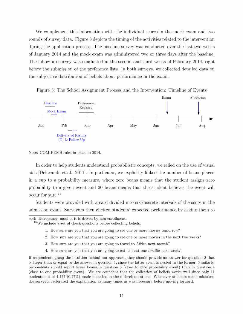
We start by showing how expected performance early in the application process compares

to actual performance in the exam. Using data from a pure control group that is not exposed

to the intervention (see Section 3.3), panel (a) of Figure 1 plots the cumulative density of the

gap between mean beliefs (see Section 3.2) and scores in the admission exam as a percentage

of the score. Approximately three quarters of the students in the pure control group expect

to perform above their actual exam score. While the average student has a 25% gap relative

to his actual admission exam score, the average gap among those with upward biased beliefs

is more than double that of students with downward biased beliefs.7

Next, we provide evidence on the potential skill mismatch that biased beliefs may generate

in terms of high-school track choices and admission outcomes. As before, we rely on data

from the control group. Panel (b) of Figure 1 reports the estimated coefficients, and the 95%

confidence intervals from regressions of preference and admission outcomes on mean beliefs

and performance in the admission exam. The results in green correspond to the regression of

the share of academic options listed, while the results in orange correspond to the regression

of admission into the academic track. Mean beliefs have a positive, albeit fairly small, effect

on students’ demand for academic schools: a one standard deviation increase in expected

test performance is associated with an average increase in the share of requested academic

options of 2.6 percentage points. On the contrary, the estimated coefficient for actual test

performance is close to zero. This pattern also holds when we focus on admission outcomes.

7Figure A.1 in Appendix shows that students with the lowest scores tend to have upwardly biased beliefswhile best performing students have mean beliefs below actual performance. Both upward and downwardbiases are observed for intermediate levels of exam score.

7

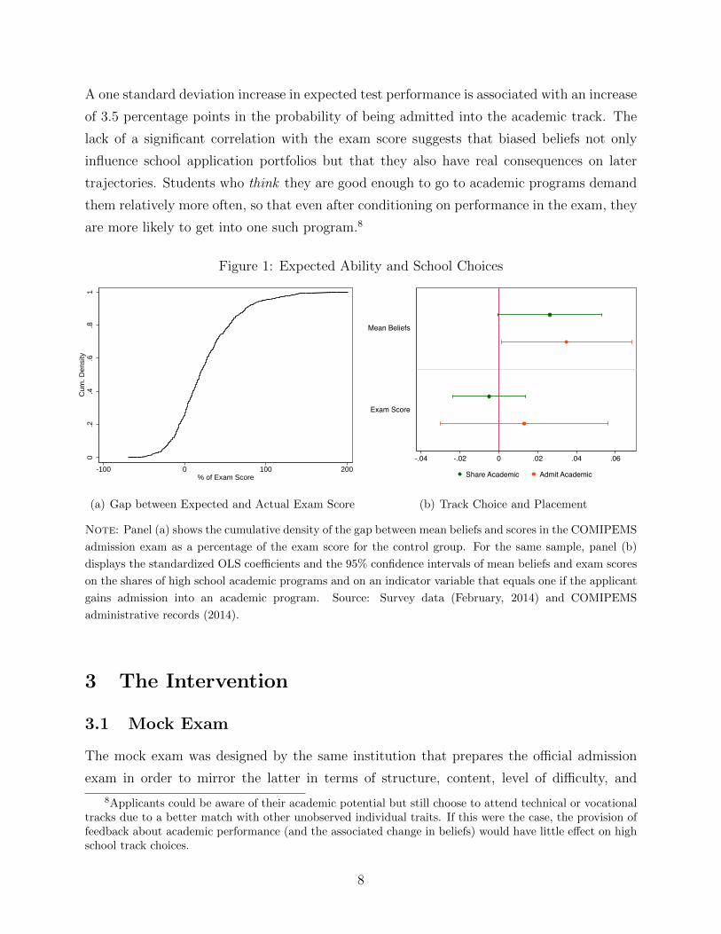
A one standard deviation increase in expected test performance is associated with an increase

of 3.5 percentage points in the probability of being admitted into the academic track. The

lack of a significant correlation with the exam score suggests that biased beliefs not only

influence school application portfolios but that they also have real consequences on later

trajectories. Students who think they are good enough to go to academic programs demand

them relatively more often, so that even after conditioning on performance in the exam, they

are more likely to get into one such program.8

Figure 1: Expected Ability and School Choices

0.2

.4.6

.81

Cum

. Den

sity

-100 0 100 200% of Exam Score

(a) Gap between Expected and Actual Exam Score

Mean Beliefs

Exam Score

-.04 -.02 0 .02 .04 .06

Share Academic Admit Academic

(b) Track Choice and Placement

Note: Panel (a) shows the cumulative density of the gap between mean beliefs and scores in the COMIPEMS

admission exam as a percentage of the exam score for the control group. For the same sample, panel (b)

displays the standardized OLS coefficients and the 95% confidence intervals of mean beliefs and exam scores

on the shares of high school academic programs and on an indicator variable that equals one if the applicant

gains admission into an academic program. Source: Survey data (February, 2014) and COMIPEMS

administrative records (2014).

3 The Intervention

3.1 Mock Exam

The mock exam was designed by the same institution that prepares the official admission

exam in order to mirror the latter in terms of structure, content, level of difficulty, and

8Applicants could be aware of their academic potential but still choose to attend technical or vocationaltracks due to a better match with other unobserved individual traits. If this were the case, the provision offeedback about academic performance (and the associated change in beliefs) would have little effect on highschool track choices.

8

duration (three hours). The exam had 128 multiple-choice questions worth one point each,

without negative marking for wrong answers.9 To reduce preparation biases due to unex-

pected testing while minimizing absenteeism, we informed students about the application of

the mock exam a few days in advance but did not tell them the exact date of the event.10

We argue that the achievement measure that we provided was easy to interpret for the

applicants while providing additional and relevant information about their academic skills.

On one hand, the intervention took place after all informative and application materials

had been distributed (see Section 2.1 and Figure 3). Those materials provide prospective

applicants with detailed information about the rules, content, structure and difficulty of the

admission exam.

On the other hand we can show that, beyond other skill measures most readily and freely

available during the application period such as the grade point average (GPA) in middle

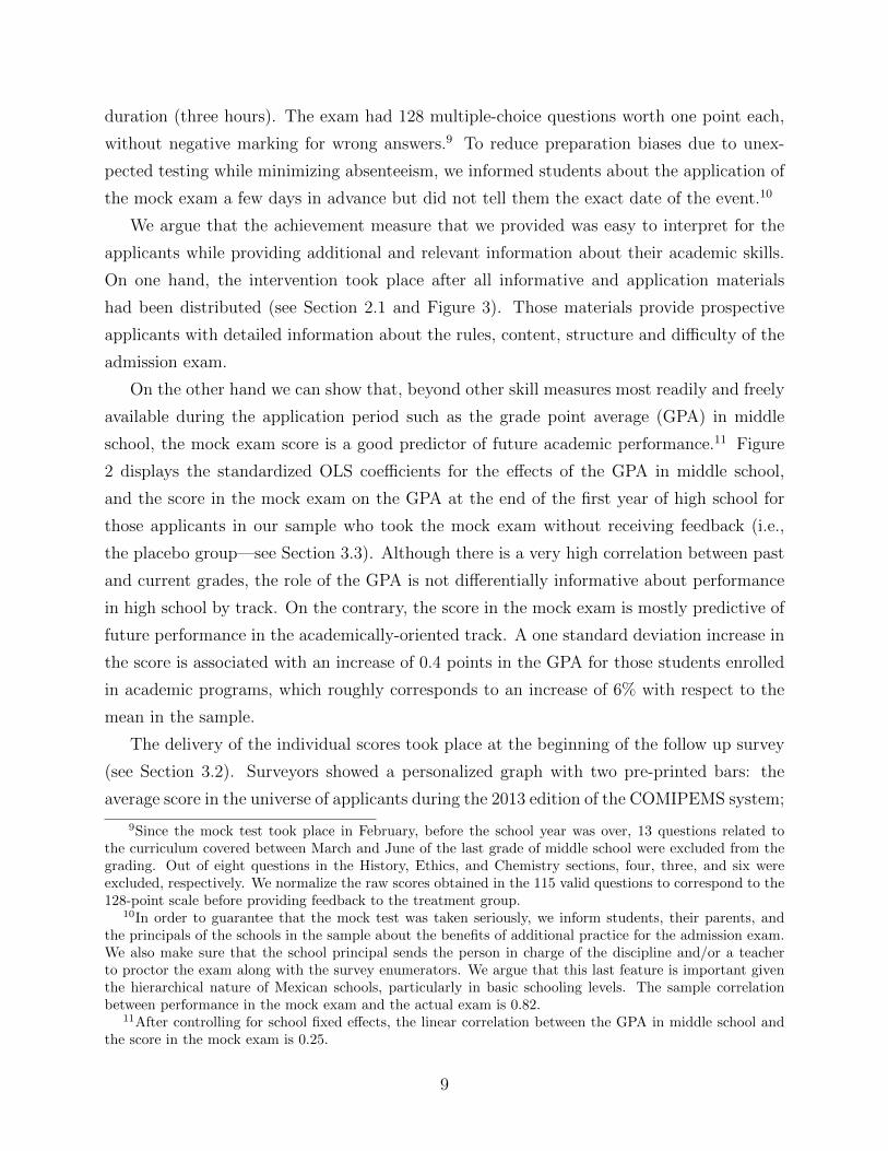
school, the mock exam score is a good predictor of future academic performance.11 Figure

2 displays the standardized OLS coefficients for the effects of the GPA in middle school,

and the score in the mock exam on the GPA at the end of the first year of high school for

those applicants in our sample who took the mock exam without receiving feedback (i.e.,

the placebo group—see Section 3.3). Although there is a very high correlation between past

and current grades, the role of the GPA is not differentially informative about performance

in high school by track. On the contrary, the score in the mock exam is mostly predictive of

future performance in the academically-oriented track. A one standard deviation increase in

the score is associated with an increase of 0.4 points in the GPA for those students enrolled

in academic programs, which roughly corresponds to an increase of 6% with respect to the

mean in the sample.

The delivery of the individual scores took place at the beginning of the follow up survey

(see Section 3.2). Surveyors showed a personalized graph with two pre-printed bars: the

average score in the universe of applicants during the 2013 edition of the COMIPEMS system;

9Since the mock test took place in February, before the school year was over, 13 questions related tothe curriculum covered between March and June of the last grade of middle school were excluded from thegrading. Out of eight questions in the History, Ethics, and Chemistry sections, four, three, and six wereexcluded, respectively. We normalize the raw scores obtained in the 115 valid questions to correspond to the128-point scale before providing feedback to the treatment group.

10In order to guarantee that the mock test was taken seriously, we inform students, their parents, andthe principals of the schools in the sample about the benefits of additional practice for the admission exam.We also make sure that the school principal sends the person in charge of the discipline and/or a teacherto proctor the exam along with the survey enumerators. We argue that this last feature is important giventhe hierarchical nature of Mexican schools, particularly in basic schooling levels. The sample correlationbetween performance in the mock exam and the actual exam is 0.82.

11After controlling for school fixed effects, the linear correlation between the GPA in middle school andthe score in the mock exam is 0.25.

9

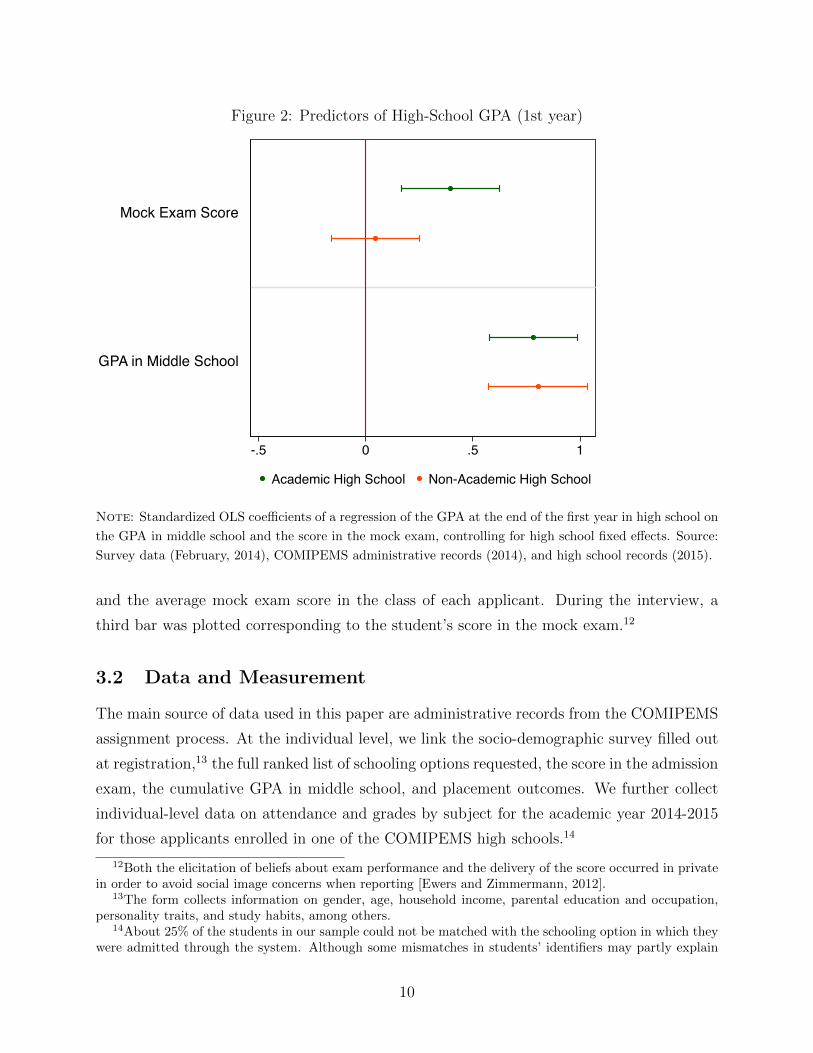
Figure 2: Predictors of High-School GPA (1st year)

Mock Exam Score

GPA in Middle School

-.5 0 .5 1

Academic High School Non-Academic High School

Note: Standardized OLS coefficients of a regression of the GPA at the end of the first year in high school on

the GPA in middle school and the score in the mock exam, controlling for high school fixed effects. Source:

Survey data (February, 2014), COMIPEMS administrative records (2014), and high school records (2015).

and the average mock exam score in the class of each applicant. During the interview, a

third bar was plotted corresponding to the student’s score in the mock exam.12

3.2 Data and Measurement

The main source of data used in this paper are administrative records from the COMIPEMS

assignment process. At the individual level, we link the socio-demographic survey filled out

at registration,13 the full ranked list of schooling options requested, the score in the admission

exam, the cumulative GPA in middle school, and placement outcomes. We further collect

individual-level data on attendance and grades by subject for the academic year 2014-2015

for those applicants enrolled in one of the COMIPEMS high schools.14

12Both the elicitation of beliefs about exam performance and the delivery of the score occurred in privatein order to avoid social image concerns when reporting [Ewers and Zimmermann, 2012].

13The form collects information on gender, age, household income, parental education and occupation,personality traits, and study habits, among others.

14About 25% of the students in our sample could not be matched with the schooling option in which theywere admitted through the system. Although some mismatches in students’ identifiers may partly explain

10

We complement this information with the individual scores in the mock exam and two

rounds of survey data. Figure 3 depicts the timing of the activities related to the intervention

during the application process. The baseline survey was conducted over the last two weeks

of January 2014 and the mock exam was administered two or three days after the baseline.

The follow-up survey was conducted in the second and third weeks of February 2014, right

before the submission of the preference lists. In both surveys, we collected detailed data on

the subjective distribution of beliefs about performance in the exam.

Figure 3: The School Assignment Process and the Intervention: Timeline of Events

JunMayAprMarFebJan

Exam

PreferenceRegistry

Delivery of Results(T) & Follow Up

Baseline

Mock Exam

Jul Aug

Allocation

Note: COMIPEMS rules in place in 2014.

In order to help students understand probabilistic concepts, we relied on the use of visual

aids [Delavande et al., 2011]. In particular, we explicitly linked the number of beans placed

in a cup to a probability measure, where zero beans means that the student assigns zero

probability to a given event and 20 beans means that the student believes the event will

occur for sure.15

Students were provided with a card divided into six discrete intervals of the score in the

admission exam. Surveyors then elicited students’ expected performance by asking them to

such discrepancy, most of it is driven by non-enrollment.15We include a set of check questions before collecting beliefs:

1. How sure are you that you are going to see one or more movies tomorrow?

2. How sure are you that you are going to see one or more movies in the next two weeks?

3. How sure are you that you are going to travel to Africa next month?

4. How sure are you that you are going to eat at least one tortilla next week?

If respondents grasp the intuition behind our approach, they should provide an answer for question 2 thatis larger than or equal to the answer in question 1, since the latter event is nested in the former. Similarly,respondents should report fewer beans in question 3 (close to zero probability event) than in question 4(close to one probability event). We are confident that the collection of beliefs works well since only 11students out of 4,127 (0.27%) made mistakes in these check questions. Whenever students made mistakes,the surveyor reiterated the explanation as many times as was necessary before moving forward.

11

allocate the 20 beans across the six intervals so as to represent the chances of scoring in each

bin.16 The survey question reads as follows (authors’ translation from Spanish):

“Suppose that you take the COMIPEMS exam today, which has a maximum

possible score of 128 and a minimum possible score of zero. How sure are you

that your score would be between ... and ...”

Assuming a uniform distribution within each interval of the score, mean beliefs are con-

structed as the summation over intervals of the product of the mid-point of the bin and the

probability assigned by the student to that bin. The variance of the distribution of beliefs

is obtained as the summation over intervals of the product of the square of the mid-point of

the bin and the probability assigned to the bin.

3.3 Sample Selection and Randomization

In order to select the experimental sample, we impose several criteria on the universe of

potential COMIPEMS applicants. First, we focus on ninth graders in general or technical

schools, excluding schooling modalities which represent a minor share of the existing educa-

tional facilities in the intervention area, such as telesecundarias. Second, we focus on schools

with a considerable mass of COMIPEMS applicants in the year 2012 (more than 30). Third,

we choose to focus on students in schools from neighborhoods with high or very high levels

of marginalization since they are the most likely to benefit from our intervention due to low

exposure to previous signals about their academic performance.17

Schools that comply with those criteria are grouped into four geographic regions (see

Figure A.2) and terciles of the school-average performance amongst ninth graders in a na-

tional standardized test aimed at measuring academic achievement (ENLACE, 2012). We

select at most 10 schools in each of the resulting 12 strata. Some strata that are less dense

participate with less schools, which explains why the final sample is comprised of 90 schools.

Whenever possible, we allow for the possibility of oversubscription of schools in each strata

in order to prevent fall backs from the sample due to implementation failures.

Treatment assignment is randomized within strata at the school level. As a result, 44

schools are assigned to the treatment group in which we administer the mock exam and

16During the pilot activities, we tested different versions with less bins and/or fewer beans. Studentsseem to be at ease manipulating 20 beans across six intervals, and hence we keep this version to reduce thecoarseness of the grid.

17Data from the 2012 edition of the assignment system shows that, on average, 33% of applicants tookany preparatory course before submitting their schooling choices. This share ranges from 44% to 12% acrossschools in neighborhoods with low and high levels marginalization, respectively.

12

provide face-to-face feedback on performance, and 46 schools are assigned to a “placebo”

group in which we only administer the mock exam, without informing about the test results.

Since compliance with the treatment assignment was perfect, the 28 over-sampled schools

constitute a pure control group that is randomized-out of the intervention and is only inter-

viewed in the follow up survey.18 Within each school in the final experimental sample, we

randomly pick one ninth grade classroom to participate in the experiment.

Our initial sample size is 3,001 students assigned to either the treatment or the placebo

group at baseline. Only 2,790 students were present on the day of the exam and a subset

of 2,544 were also present in the follow up survey. Since the actual treatment was only

delivered at the end of the follow up survey, feedback provision does not generate differential

attrition patterns. Adding the 912 students from the control group yields a sample of 3,456

observations with complete survey and exam records. The final sample consists of 3,100

students who can be matched with the COMIPEMS administrative data.19

3.4 Descriptives

Table A.1 provides basic descriptive statistics and a balancing test of the randomization for

the main variables used in the empirical analysis. Consistent with the random treatment

assignment, no significant differences are detected across groups. Before the intervention,

about 30% of the students in our sample had taken at least one COMIPEMS mock exam and

roughly half of these had received feedback about their performance therein. By the time

of the submission of the preference lists, approximately half of the students had attended

preparatory courses for the admission exam. About a third declared themselves to be working

(either paid or unpaid), and only 12% have parents with complete higher education. Almost

70% of the students in our sample plan to go to college.

The median student in the placebo group applies to 10 schooling options, slightly fewer

than 10% of the applicants in that group request less than five options while under 2% fill

all of the 20 school slots. The average portfolio share of academic options is 51%, while the

average share of technical and vocational options are 37% and 12%, respectively. Roughly

two thirds of the applicants are assigned to a school within their top four choices.

About 14% of the applicants in the placebo group remain unplaced after the matching

algorithm described in Section 2.1, and 3% are subsequently admitted into one of the school-

ing options with remaining slots available. Among placed applicants, 47% are admitted into

18As shown in Figure A.2, some strata are not populated for this group.19The 10% discrepancy between the survey data and the administrative data reflects applicants’ partici-

pation decisions in the COMIPEMS system.

13

a school from the academic track, 36% gain admission into the technical track and the re-

maining 17% gain admission into the vocational track. The vast majority of the applicants

in the placebo group are assigned to a high school that is located in the same State as their

middle school (93% in the Federal District and 79% in the State of Mexico), indicating a

large degree of segmentation across the two schooling markets.

High school records for the placebo group reveal that enrollment conditional on assign-

ment does not vary across tracks, although it is much higher in the Federal District than in

the State of Mexico. While 87% of the applicants who are initially assigned to a school in

the Federal District enroll in that school, only 68% of the applicants in the State of Mexico

do so.20 Among enrolled applicants in the placebo group, we find that 14% drop out and

19% are held back during the first year of high school. Dropout rates are relatively higher

(24%) in the vocational track.

4 A Bayesian Learning Model

4.1 Belief Updating

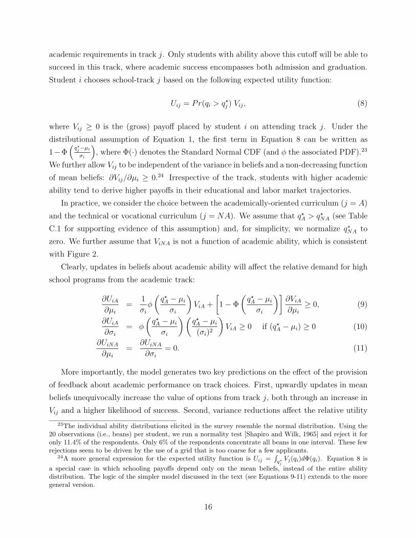
Academic ability is a draw qi from an individual-specific distribution:21

qi ∼ N(µi, σ2i ). (1)

Students do not observe their own ability directly, although they know its underlying dis-

tribution. Measures of academic performance (e.g., school grades, standardized test scores)

and other types of feedback (from teachers, peers, parents, etc.) provide students with noisy

signals si about qi:

si = qi + εi

where εi ∼ N(0, σ2ε ).

22 We assume that each signal leads agents to update their beliefs in a

20The lower enrollment rates in the State of Mexico are in part due to the access to other public schoolsoutside the COMIPEMS process.

21We take as given the first and second moments of the individual distribution of ability at a certainpoint in time. After controlling for actual test performance, mean beliefs in the baseline survey correlatepositively and significantly with the GPA in middle school, the reported weekly hours of homework study,one personality trait that proxies perseverance, a composite wealth-index based on household durable goods,a dummy for whether or not applicants expect to attend college and an index of students’ subjective rankingin their class. No systematic relationship is found with respect to the gender of the applicants.

22In practice, the perceived noisiness of each signal may vary across individuals. We do not considerthis source of heterogeneity in the model to the extent that it is not observable in the data and it does notsystematically alter any of the predictions.

14

Bayesian fashion:

µ′

i = E(qi|si) = µi + (si − µi)σ2i

(σ2i + σ2

ε )(2)

σ2′

i = V ar(qi|si) =

[1− σ2

i

(σ2i + σ2

ε )

]σ2i . (3)

The sign of (si− µi) in Equation 2 determines the direction of the update, e.g., students

who perform better than expected update their mean beliefs upwards while those who do

worse than expected adjust their mean beliefs downwards. Henceforth, we refer to students

who score higher than they expected as “upward-updaters” and label students who did worse

than they expected as “downward-updaters”. Equation 3 shows that the posterior variance

σ2′i is independent of the direction of the update, and depends on the value of σ2

ε relative to

σ2i . For instance, a signal that is as noisy as the prior distribution of beliefs (i.e., σ2

ε = σ2i )

halves the variance of the prior regardless of the value of si.

Although every signal generates an update, the magnitude of the change in posterior

beliefs depends on individual priors according to the following expressions:

∂µ′i

∂µi= 1− σ2

i

(σ2i + σ2

ε )≥ 0 (4)

∂µ′i

∂σ2i

= (si − µi)[

σ2ε

(σ2i + σ2

ε )2

]≥ 0 if (si − µi) ≥ 0 (5)

∂σ2′i

∂µi= 0 (6)

∂σ2′i

∂σ2i

=σ4ε

(σ2i + σ2

ε )2≥ 0. (7)

Equations 4 and 7 show that there is a monotonic positive relationship between priors

and posteriors for both moments of the ability distribution. Equation 5 reveals that the

dispersion in the priors plays a role in the determination of mean posteriors, and that this

effect depends on the realization of the signal relative to mean priors. Noisier priors lead

to higher (lower) mean posteriors among those who perform better (worse) than expected.

Equation 6 implies that mean priors do not mediate the updating process in the variance.

4.2 Track Choices

Based on beliefs about their own ability, students make choices about the schooling curricu-

lum they wish to attend. Let q?j be the minimum ability cutoff required to comply with the

15

academic requirements in track j. Only students with ability above this cutoff will be able to

succeed in this track, where academic success encompasses both admission and graduation.

Student i chooses school-track j based on the following expected utility function:

Uij = Pr(qi > q?j ) Vij, (8)

where Vij ≥ 0 is the (gross) payoff placed by student i on attending track j. Under the

distributional assumption of Equation 1, the first term in Equation 8 can be written as

1−Φ(q?j−µiσi

), where Φ(·) denotes the Standard Normal CDF (and φ the associated PDF).23

We further allow Vij to be independent of the variance in beliefs and a non-decreasing function

of mean beliefs: ∂Vij/∂µi ≥ 0.24 Irrespective of the track, students with higher academic

ability tend to derive higher payoffs in their educational and labor market trajectories.

In practice, we consider the choice between the academically-oriented curriculum (j = A)

and the technical or vocational curriculum (j = NA). We assume that q?A > q?NA (see Table

C.1 for supporting evidence of this assumption) and, for simplicity, we normalize q∗NA to

zero. We further assume that ViNA is not a function of academic ability, which is consistent

with Figure 2.

Clearly, updates in beliefs about academic ability will affect the relative demand for high

school programs from the academic track:

∂UiA∂µi

=1

σiφ

(q?A − µiσi

)ViA +

[1− Φ

(q?A − µiσi

)]∂ViA∂µi

≥ 0, (9)

∂UiA∂σi

= φ

(q?A − µiσi

)(q?A − µi

(σi)2

)ViA ≥ 0 if (q?A − µi) ≥ 0 (10)

∂UiNA∂µi

=∂UiNA∂σi

= 0. (11)

More importantly, the model generates two key predictions on the effect of the provision

of feedback about academic performance on track choices. First, upwardly updates in mean

beliefs unequivocally increase the value of options from track j, both through an increase in

Vij and a higher likelihood of success. Second, variance reductions affect the relative utility

23The individual ability distributions elicited in the survey resemble the normal distribution. Using the20 observations (i.e., beans) per student, we run a normality test [Shapiro and Wilk, 1965] and reject it foronly 11.4% of the respondents. Only 6% of the respondents concentrate all beans in one interval. These fewrejections seem to be driven by the use of a grid that is too coarse for a few applicants.

24A more general expression for the expected utility function is Uij =∫q?jVj(qi)dΦ(qi). Equation 8 is

a special case in which schooling payoffs depend only on the mean beliefs, instead of the entire abilitydistribution. The logic of the simpler model discussed in the text (see Equations 9-11) extends to the moregeneral version.

16

of academic track options only through an effect on the likelihood of success. However, this

effect depends on the location of the mean posterior relative to q∗A. That is, changes in the

dispersion of the ability distribution enabled by the receipt of the signal can either reinforce

or counteract the effect of updates in mean beliefs. In sum, the net effect of the signal on

the demand for academic programs depends on the location of µ′i relative to q∗A.

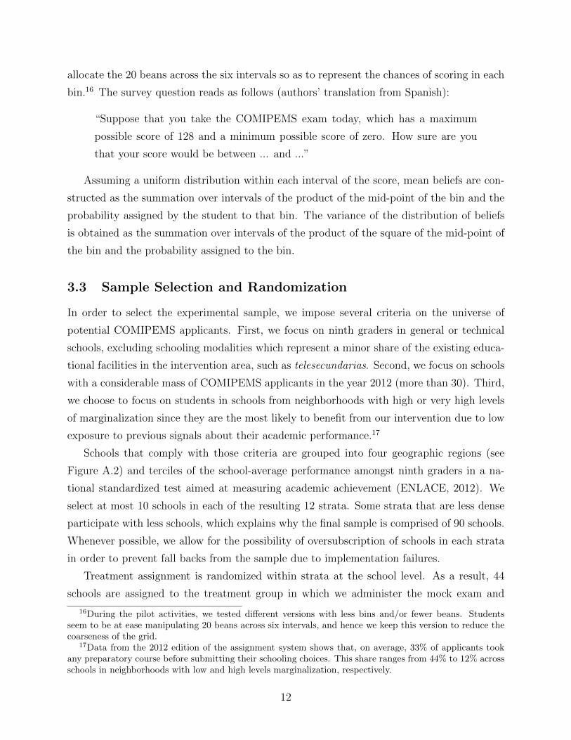
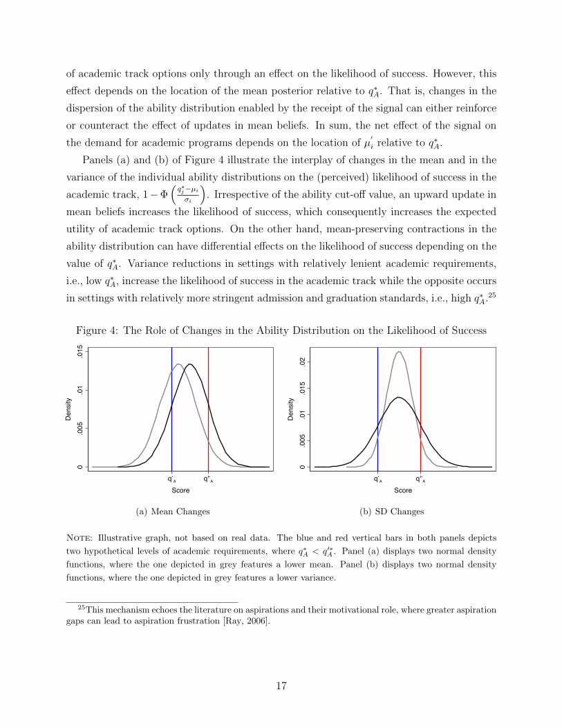
Panels (a) and (b) of Figure 4 illustrate the interplay of changes in the mean and in the

variance of the individual ability distributions on the (perceived) likelihood of success in the

academic track, 1−Φ(q?j−µiσi

). Irrespective of the ability cut-off value, an upward update in

mean beliefs increases the likelihood of success, which consequently increases the expected

utility of academic track options. On the other hand, mean-preserving contractions in the

ability distribution can have differential effects on the likelihood of success depending on the

value of q∗A. Variance reductions in settings with relatively lenient academic requirements,

i.e., low q∗A, increase the likelihood of success in the academic track while the opposite occurs

in settings with relatively more stringent admission and graduation standards, i.e., high q∗A.25

Figure 4: The Role of Changes in the Ability Distribution on the Likelihood of Success

0.005

.01

.015

Density

q*A q'*AScore

(a) Mean Changes

0.005

.01

.015

.02

Density

q*A q'*AScore

(b) SD Changes

Note: Illustrative graph, not based on real data. The blue and red vertical bars in both panels depicts

two hypothetical levels of academic requirements, where q∗A < q′∗A . Panel (a) displays two normal density

functions, where the one depicted in grey features a lower mean. Panel (b) displays two normal density

functions, where the one depicted in grey features a lower variance.

25This mechanism echoes the literature on aspirations and their motivational role, where greater aspirationgaps can lead to aspiration frustration [Ray, 2006].

17

5 Empirical Evidence

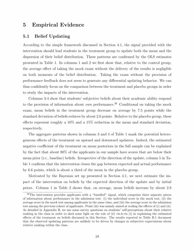
5.1 Belief Updating

According to the simple framework discussed in Section 4.1, the signal provided with the

intervention should lead students in the treatment group to update both the mean and the

dispersion of their belief distribution. These patterns are confirmed by the OLS estimates

presented in Table 1. In columns 1 and 2 we first show that, relative to the control group,

the average effect of taking the mock exam without the delivery of the results is negligible

on both moments of the belief distribution. Taking the exam without the provision of

performance feedback does not seem to generate any differential updating behavior. We can

thus confidently focus on the comparison between the treatment and placebo groups in order

to study the impacts of the intervention.

Columns 3-4 show that students’ subjective beliefs about their academic ability respond

to the provision of information about own performance.26 Conditional on taking the mock

exam, mean beliefs in the treatment group decrease on average by 7.5 points while the

standard deviation of beliefs reduces by about 2.6 points. Relative to the placebo group, these

effects represent roughly a 10% and a 15% reduction in the mean and standard deviation,

respectively.

The aggregate patterns shown in columns 3 and 4 of Table 1 mask the potential hetero-

geneous effects of the treatment on upward and downward updaters. Indeed, the estimated

negative coefficient of the treatment on mean posteriors in the full sample can be explained

by the fact that about 80% of the applicants in our sample have scores that are below their

mean prior (i.e., baseline) beliefs. Irrespective of the direction of the update, column 5 in Ta-

ble 1 confirms that the intervention closes the gap between expected and actual performance

by 6.6 points, which is about a third of the mean in the placebo group.

Motivated by the Bayesian set up presented in Section 4.1, we next estimate the im-

pact of the intervention on beliefs by the expected direction of the update and by initial

priors. Column 1 in Table 2 shows that, on average, mean beliefs increase by about 2.8

26The intervention provides applicants with a “bundled” signal, which comprises three separate piecesof information about performance in the admission test: (i) the individual score in the mock test, (ii) theaverage score in the mock test among applicants in the same class, and (iii) the average score in the admissiontest among the previous cohort of applicants. Point (iii) was mainly aimed at scaling the effects of (i) and (ii).As detailed in Appendix B, we use some survey questions on students’ self-perceptions about their relativeranking in the class in order to shed some light on the role of (ii) vis-a-vis (i) in explaining the estimatedeffects of the treatment on beliefs discussed in this Section. The results reported in Table B.1 documentthat the observed updating patterns are unlikely to be driven by changes in subjective expectations aboutrelative ranking within the class.

18

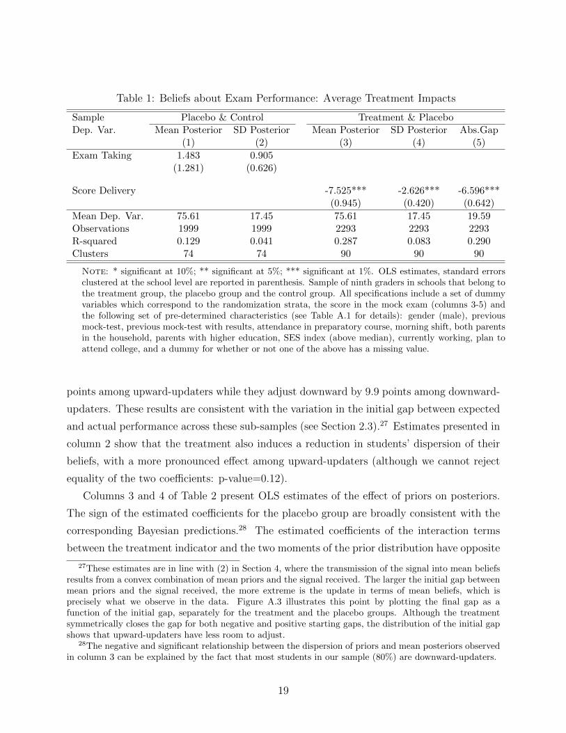
Table 1: Beliefs about Exam Performance: Average Treatment Impacts

Sample Placebo & Control Treatment & PlaceboDep. Var. Mean Posterior SD Posterior Mean Posterior SD Posterior Abs.Gap

(1) (2) (3) (4) (5)

Exam Taking 1.483 0.905(1.281) (0.626)

Score Delivery -7.525*** -2.626*** -6.596***(0.945) (0.420) (0.642)

Mean Dep. Var. 75.61 17.45 75.61 17.45 19.59Observations 1999 1999 2293 2293 2293R-squared 0.129 0.041 0.287 0.083 0.290Clusters 74 74 90 90 90

Note: * significant at 10%; ** significant at 5%; *** significant at 1%. OLS estimates, standard errorsclustered at the school level are reported in parenthesis. Sample of ninth graders in schools that belong tothe treatment group, the placebo group and the control group. All specifications include a set of dummyvariables which correspond to the randomization strata, the score in the mock exam (columns 3-5) andthe following set of pre-determined characteristics (see Table A.1 for details): gender (male), previousmock-test, previous mock-test with results, attendance in preparatory course, morning shift, both parentsin the household, parents with higher education, SES index (above median), currently working, plan toattend college, and a dummy for whether or not one of the above has a missing value.

points among upward-updaters while they adjust downward by 9.9 points among downward-

updaters. These results are consistent with the variation in the initial gap between expected

and actual performance across these sub-samples (see Section 2.3).27 Estimates presented in

column 2 show that the treatment also induces a reduction in students’ dispersion of their

beliefs, with a more pronounced effect among upward-updaters (although we cannot reject

equality of the two coefficients: p-value=0.12).

Columns 3 and 4 of Table 2 present OLS estimates of the effect of priors on posteriors.

The sign of the estimated coefficients for the placebo group are broadly consistent with the

corresponding Bayesian predictions.28 The estimated coefficients of the interaction terms

between the treatment indicator and the two moments of the prior distribution have opposite

27These estimates are in line with (2) in Section 4, where the transmission of the signal into mean beliefsresults from a convex combination of mean priors and the signal received. The larger the initial gap betweenmean priors and the signal received, the more extreme is the update in terms of mean beliefs, which isprecisely what we observe in the data. Figure A.3 illustrates this point by plotting the final gap as afunction of the initial gap, separately for the treatment and the placebo groups. Although the treatmentsymmetrically closes the gap for both negative and positive starting gaps, the distribution of the initial gapshows that upward-updaters have less room to adjust.

28The negative and significant relationship between the dispersion of priors and mean posteriors observedin column 3 can be explained by the fact that most students in our sample (80%) are downward-updaters.

19

Table 2: Beliefs about Exam Performance: Heterogeneous Treatment Impacts

Sample Treatment & PlaceboDependent Variable Mean Posterior SD Posterior Mean Posterior SD Posterior

(1) (2) (3) (4)

Treat×(Upward Updater) 2.786** -3.623***(1.317) (0.766)

Treat×(Downward Updater) -9.854*** -2.423***(0.915) (0.428)

Upward Updater -14.533*** 3.104***(1.135) (0.601)

Treatment 5.118 -0.042(4.136) (2.269)

Treat×(Mean Prior) -0.194*** 0.002(0.042) (0.022)

Mean Prior 0.523*** -0.005(0.039) (0.015)

Treat×(SD Prior) 0.121* -0.148***(0.065) (0.055)

SD Prior -0.101** 0.591***(0.047) (0.040)

Mean Dependent Variable 75.61 17.45 75.61 17.45Number of Observations 2293 2293 2293 2293R-squared 0.346 0.095 0.429 0.368Number of Clusters 90 90 90 90

Note: * significant at 10%; ** significant at 5%; *** significant at 1%. OLS estimates, standard errorsclustered at the school level are reported in parenthesis. Sample of ninth graders in schools that belong tothe treated and the placebo group. Downward (upward) updaters are defined as those with mean baselinebeliefs that are higher (lower) than the realized value of the score in the mock exam. All specificationsinclude a set of dummy variables which correspond to the randomization strata, the score in the mockexam and the following set of pre-determined characteristics (see Table A.1 for details): gender (male),previous mock-test, previous mock-test with results, attendance in preparatory course, morning shift,both parents in the household, parents with higher education, SES index (above median), currentlyworking, plan to attend college, and a dummy for whether or not one of the above has a missing value.

signs when compared to the coefficients on priors. That is, the signal provided through the

intervention reduces the dependence of posteriors on priors. This is particularly beneficial for

the applicants in our sample, who appear to be quite inaccurate in their initial predictions

(see Panel (a) of Figure 1).

20

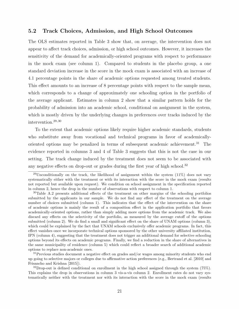
5.2 Track Choices, Admission, and High School Outcomes

The OLS estimates reported in Table 3 show that, on average, the intervention does not

appear to affect track choices, admission, or high school outcomes. However, it increases the

sensitivity of the demand for academically-oriented programs with respect to performance

in the mock exam (see column 1). Compared to students in the placebo group, a one

standard deviation increase in the score in the mock exam is associated with an increase of

4.1 percentage points in the share of academic options requested among treated students.

This effect amounts to an increase of 8 percentage points with respect to the sample mean,

which corresponds to a change of approximately one schooling option in the portfolio of

the average applicant. Estimates in column 2 show that a similar pattern holds for the

probability of admission into an academic school, conditional on assignment in the system,

which is mostly driven by the underlying changes in preferences over tracks induced by the

intervention.29,30

To the extent that academic options likely require higher academic standards, students

who substitute away from vocational and technical programs in favor of academically-

oriented options may be penalized in terms of subsequent academic achievement.31 The

evidence reported in columns 3 and 4 of Table 3 suggests that this is not the case in our

setting. The track change induced by the treatment does not seem to be associated with

any negative effects on drop-out or grades during the first year of high school.32

29Unconditionally on the track, the likelihood of assignment within the system (11%) does not varysystematically either with the treatment or with its interaction with the score in the mock exam (resultsnot reported but available upon request). We condition on school assignment in the specification reportedin column 2, hence the drop in the number of observations with respect to column 1.

30Table A.2 presents additional effects of the treatment on other margins of the schooling portfoliossubmitted by the applicants in our sample. We do not find any effect of the treatment on the averagenumber of choices submitted (column 1). This indicates that the effect of the intervention on the shareof academic options is mainly the result of a composition effect in the application portfolio that favorsacademically-oriented options, rather than simply adding more options from the academic track. We alsodiscard any effects on the selectivity of the portfolio, as measured by the average cutoff of the optionssubmitted (column 2). We do find a small and significant effect on the share of UNAM options (column 3),which could be explained by the fact that UNAM schools exclusively offer academic programs. In fact, thiseffect vanishes once we incorporate technical options sponsored by the other university affiliated institution,IPN (column 4), suggesting that the treatment does not trigger an additional demand for selective schoolingoptions beyond its effects on academic programs. Finally, we find a reduction in the share of alternatives inthe same municipality of residence (column 5) which could reflect a broader search of additional academicoptions to replace non-academic ones.

31Previous studies document a negative effect on grades and/or wages among minority students who endup going to selective majors or colleges due to affirmative action preferences (e.g., Bertrand et al. [2010] andFrisancho and Krishna [2015]).

32Drop-out is defined conditional on enrollment in the high school assigned through the system (75%).This explains the drop in observations in column 3 vis-a-vis column 2. Enrollment rates do not vary sys-tematically neither with the treatment nor with its interaction with the score in the mock exam (results

21

Table 3: Track Choices, Admission, and High School Outcomes

Sample Treatment & PlaceboDependent Variable Share Admission High School High School

Academic Academic Drop-out GPA(1) (2) (3) (4)

Treatment× Mock Exam Score 0.041*** 0.059** -0.012 -0.049(0.013) (0.027) (0.021) (0.072)

Treatment 0.012 -0.026 0.025 -0.037(0.016) (0.026) (0.024) (0.069)

Mock Exam Score (z-score) -0.016* 0.004 -0.034* 0.336***(0.009) (0.022) (0.018) (0.049)

Mean Dependent Variable 0.518 0.477 0.148 7.662Number of Observations 2293 2045 1529 1302R-squared 0.087 0.067 0.380 0.440Number of Clusters 90 90 90 90

Note: * significant at 10%; ** significant at 5%; *** significant at 1%. OLS estimates, standard errorsclustered at the school level are reported in parenthesis. Sample of ninth graders (columns 1 and 2)and tenth graders (columns 3 and 4) that are assigned to the treatment and the placebo group. Allspecifications include a set of dummy variables which correspond to the randomization strata, the scorein the mock exam and the following set of pre-determined characteristics (see Table A.1 for details):gender (male), previous mock-test, previous mock-test with results, attendance in preparatory course,morning shift, both parents in the household, parents with higher education, SES index (above median),currently working, plan to attend college, and a dummy for whether or not one of the above has a missingvalue. The specifications in columns 3 and 4 further include fixed effects at the high school level.

6 Mechanisms

6.1 Belief Updating and Track Choices

The simple framework exposed in Section 4.2 suggests that changes in the first and the

second moments of the ability distribution interact to determine high school track choices.

This prediction has key implications for understanding the schooling responses of the infor-

mational intervention. Since the treatment induces a reduction in the variance of the ability

distributions (see Tables 1 and 2), any increase (decrease) in the demand for academic pro-

grams resulting from higher (lower) mean beliefs is most likely reinforced (counteracted) in

settings with more lenient requirements. Conversely, any positive (negative) shock on mean

beliefs is counteracted (reinforced) in settings where those requirements are more stringent.

not reported but available upon request). The GPA in high school is not observed for drop-outs (15%),hence the difference in the number of observations between columns 3 and 4. In order to take into accountschool-specific trends in high school outcomes, we include high school fixed effects in columns 3 and 4.

22

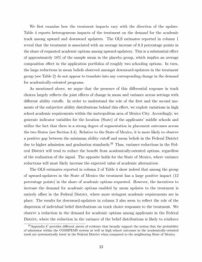
We first examine how the treatment impacts vary with the direction of the update.

Table 4 reports heterogeneous impacts of the treatment on the demand for the academic

track among upward and downward updaters. The OLS estimates reported in column 1

reveal that the treatment is associated with an average increase of 8.3 percentage points in

the share of requested academic options among upward-updaters. This is a substantial effect

of approximately 18% of the sample mean in the placebo group, which implies an average

composition effect in the application portfolios of roughly two schooling options. In turn,

the large reductions in mean beliefs observed amongst downward-updaters in the treatment

group (see Table 2) do not appear to translate into any corresponding change in the demand

for academically-oriented programs.

As mentioned above, we argue that the presence of this differential response in track

choices largely reflects the joint effects of change in mean and variance across settings with

different ability cutoffs. In order to understand the role of the first and the second mo-

ments of the subjective ability distributions behind this effect, we exploit variations in high

school academic requirements within the metropolitan area of Mexico City. Accordingly, we

generate indicator variables for the location (State) of the applicants’ middle schools and

utilize the fact that there is a strong degree of segmentation in placement outcomes across

the two States (see Section 3.4). Relative to the State of Mexico, it is more likely to observe

a positive gap between the minimum ability cutoff and mean beliefs in the Federal District

due to higher admission and graduation standards.33 Thus, variance reductions in the Fed-

eral District will tend to reduce the benefit from academically-oriented options, regardless

of the realization of the signal. The opposite holds for the State of Mexico, where variance

reductions will most likely increase the expected value of academic alternatives.

The OLS estimates reported in column 2 of Table 4 show indeed that among the group

of upward-updaters in the State of Mexico the treatment has a large positive impact (12

percentage points) in the share of academic options requested. However, the incentives to

increase the demand for academic options enabled by mean updates to the treatment is

entirely offset in the Federal District, where more stringent academic requirements are in

place. The results for downward-updaters in column 3 also seem to reflect the role of the

dispersion of individual belief distributions on track choice responses to the treatment. We

observe a reduction in the demand for academic options among applicants in the Federal

District, where the reduction in the variance of the belief distributions is likely to reinforce

33Appendix C provides different pieces of evidence that broadly support the notion that the probabilityof admission within the COMIPEMS system as well as high school outcomes in the academically-orientedtrack are systematically lower in the Federal District when compared to the neighboring State of Mexico.

23

Table 4: Belief Updating and High School Track Choices

Dependent Variable Share of Academic SchoolsSample All Upward-

updatersDownward-

updaters(1) (2) (3)

Treatment×(Upward-updater) 0.083***(0.029)

Treatment×(Downward-updater) -0.005(0.017)

Upward-updater -0.057**(0.022)

Treatment 0.120*** 0.019(0.033) (0.020)

Treatment×(Federal District) -0.118* -0.084***(0.061) (0.030)

Federal District 0.149** -0.050(0.068) (0.031)

Mean Dependent Variable 0.51 0.46 0.52Number of Observations 2293 441 1852R-squared 0.086 0.171 0.092Number of Clusters 90 84 90

Note: * significant at 10%; ** significant at 5%; *** significant at 1%. OLS estimates, standard errorsclustered at the school level are reported in parenthesis. Sample of ninth graders in schools that belong tothe treated and placebo groups. Downward-(upward) updaters are defined as those with mean baselinebeliefs that are higher (lower) than the realized value of the score in the mock exam. All specificationsinclude a set of dummy variables which correspond to the randomization strata, the score in the mockexam and the following set of pre-determined characteristics (see Table A.1 for details): gender (male),previous mock-test, previous mock-test with results, attendance in preparatory course, morning shift,both parents in the household, parents with higher education, SES index (above median), currentlyworking, plan to attend college, and a dummy for whether or not one of the above has a missing value.

the effect of changes in mean beliefs.34

The observed differential response to the treatment reported in column 1 of Table 4 can

34Table A.3 checks if the null impact on the number of options of the portfolio persists when we look atthe differential treatment effects by the direction of the update and location. Indeed, the number of optionslisted is unaffected even if we look at the differential effect by direction of the update (column 1) or by thedirection of the update and by location (column 2). In general, this implies that the result of substitutionof options across tracks holds.

24

thus be explained, to a large extent, by a composition effect. Since approximately three

quarters of the applicants in the sample reside in the State of Mexico, the previous result

most likely reflects the reinforcing effect of the variance among upward updaters and its

corresponding counteracting effect for downward-updaters in this location.

6.2 Dealing with the Endogeneity of Beliefs

The empirical relationship between beliefs and choices is contaminated by unobserved het-

erogeneity. Individuals with greater confidence, for example, may have higher expected

academic ability and tend to demand more academic options. Thus, simply regressing the

share of academic options requested on observed belief posteriors is unlikely to be informative

in terms of the effect of the mean and the dispersion of the subjective ability distributions

on track choices.

Our intervention allows us to generate instrumental variables for actual posteriors based

on the predictions of the Bayesian model. Given the score in the mock exam, we can

construct predicted posteriors based on the priors of each student.35 These are plausibly

credible instruments since: (i) the Bayesian predictions for both the mean and the dispersion

of the ability distribution are highly correlated with their observed counterparts (particularly

amongst the group of students who receive feedback on their performance); and (ii) they are

likely to affect choices only through the corresponding changes in beliefs induced by the

intervention.

Given the same observed posteriors, applicants in the treatment group should exhibit

a better alignment of their academic ability with the share of academic options requested.

That is, the coefficient of the interaction term between the predicted mean posteriors and the

treatment indicator should be positive. In turn, the sign of the coefficient of the interaction

term between the treatment indicator and the predicted standard deviation of the posterior

depends on the rigidity of the academic requirements in the location of residence. For

example, the same observed dispersion of the posterior is likely to be associated with a

reduction in the share of academic options among applicants in the treatment group in the

Federal District. Given that (q∗A − µi) is more likely to be positive in this setting, the drop

35We impute missing values for 122 observations with zero variance at baseline, which roughly correspondsto 5% of the sample (balanced between the treatment and the placebo groups). We input σ2

i based on theaverage of the empirical belief distributions at baseline and make some assumptions on σ2

ε to construct thetheoretical moments predicted by the Bayesian benchmark. In particular, we impose an upper bound andset σ2

ε to the value of the variance of the residual that results from regressing the mock exam score on thesame set of individual, household, and school characteristics that we use as control variables throughout theanalysis (see Table A.1 for details).

25

Table 5: The Effects of (Bayesian) Beliefs on High School Track Choices

Sample Treatment & PlaceboDependent Variable Mean SD Share

Posterior Posterior AcademicEstimator OLS OLS 2SLS

(1) (2) (3)

Bayesian Mean Posterior 0.648*** -0.027(0.052) (0.020)

(Bayesian SD Posterior) × (Federal District) 0.572*** 1.191***(0.157) (0.105)

(Bayesian SD Posterior) × (Mexico State) 0.392*** 1.266***(0.131) (0.085)

Treatment × (Mean Posterior) 0.047**(0.024)

Mean Posterior -0.000(0.002)

Treatment × (SD Posterior) × (Federal District) -0.008***(0.003)

Treatment × (SD Posterior) × (Mexico State) -0.002(0.003)

(SD Posterior) × (Federal District) 0.000(0.003)

(SD Posterior) × (Mexico State) 0.001(0.002)

Treatment 0.076(0.054)

Mean Dependent Variable 72.45 16.61 0.52Number of Observations 2171 2171 2171R-squared 0.334 0.281 0.085Number of Clusters 90 90 90Weak IV Test:Kleibergen-Paap Chi-sq (p-value) 49.68

(0.000)

Note: * significant at 10%; ** significant at 5%; *** significant at 1%. OLS and 2SLS estimates,standard errors clustered at the school level are reported in parenthesis. Sample of ninth graders inschools that belong to the treated and placebo groups. All specifications include a set of dummy variableswhich correspond to the randomization strata. the score in the mock exam and the following set ofpre-determined characteristics (see Table A.1 for details): gender (male), previous mock-test, previousmock-test with results, attendance in preparatory course, morning shift, both parents in the household,parents with higher education, SES index (above median), currently working, plan to attend college, anda dummy for whether or not one of the above has a missing value.

26

in variance will reduce the value of academic options (see Equation 10).

Table 5 presents the resulting estimates. Columns 1 and 2 display the first-stage OLS

coefficients of observed posteriors on Bayesian posteriors, which confirms a robust and sys-

tematic relationship between the two.36 Column 3 presents the corresponding 2SLS esti-

mates, whereby the observed posteriors are instrumented with their Bayesian counterparts.

The estimated coefficient of the interaction effect between the treatment and mean posteri-

ors is positive. The triple interaction effect between the treatment indicator, the standard

deviations posteriors, and the indicator variable for the Federal District confirms that the

treatment-induced reduction in variance leads to a reduction in the share of academic options

in this setting.

6.3 Other Schooling Responses

Beyond the school choices submitted within the assignment system, the process of belief up-

dating induced by the treatment may trigger other behavioral responses of potential interest.

For instance, it is likely that the observed changes in the perceived ability distributions may

influence students’ motivation to prepare for the exam. Here we provide some evidence

in favor of this channel by examining the effects of the treatment on performance in the

admission exam.37

Column 1 in Table 6 displays the estimated treatment impacts on individual scores in

the admission exam by the expected direction of the update. While there seems to be

no discernible effect on test scores among upward-updaters, downward-updaters have lower

scores by approximately 10% of a standard deviation with respect to the placebo group. In

line with the results discussed in Section 6.1, the discouragement effect of the intervention

on subsequent study effort varies depending on the stringency of the academic requirements

between States. In particular, the negative effect on effort appears to be concentrated among

applicants from the Federal District who experience a reduction of about 37% of a standard

deviation of the score in the admission exam (see column 3).

The evidence reported here is consistent with the results discussed in Sections 6.1 and 6.2

as to the interplay between variance reductions and mean changes in the ability distribution

enabled by the information intervention.38

36Figure A.4 displays the empirical relationship between the observed and predicted posteriors in thetreatment group.

37A very small number (38) of applicants submit their preferences in the system but do not take theadmission exam. This share corresponds to 1.6% of the sample, and it does not vary systematically witheither the expected direction of the update or with the stringency of the academic requirements across States.

38Columns 4 and 6 of Table A.3 in Appendix A show a negative effect of the treatment on the preferences

27

Table 6: Belief Updating and Study Effort

Dependent Variable Standardized Score in the Admission ExamSample All Upward-

updatersDownward-

updaters(1) (2) (3)

Treatment × (Upward-updater) -0.068(0.056)

Treatment × (Downward-updater) -0.095**(0.043)

Upward-updater -0.094**(0.043)

Treatment -0.075 -0.005(0.065) (0.042)

Treatment × (Federal District) -0.093 -0.368***(0.125) (0.094)

Federal District 0.060 0.214**(0.103) (0.097)

Mean Dependent Variable 0.02 0.71 -0.12Number of Observations 2253 437 1816R-squared 0.713 0.750 0.659Number of Clusters 90 84 90

Note: * significant at 10%; ** significant at 5%; *** significant at 1%. OLS estimates, standard errorsclustered at the school level are reported in parenthesis. Sample of ninth graders in schools that belongto the treated and placebo groups. Downward-(upward)updaters are defined as those with mean baselinebeliefs that are higher (lower) than the realized value of the score in the mock exam. All specificationsinclude a set of dummy variables which correspond to the randomization strata, the score in the mockexam and the following set of pre-determined characteristics (see Table A.1 for details): gender (male),previous mock-test, previous mock-test with results, attendance in preparatory course, morning shift,both parents in the household, parents with higher education, SES index (above median), currentlyworking, plan to attend college, and a dummy for whether or not one of the above has a missing value.

over school selectivity among downward-updaters from the Federal District. These findings offer furtherevidence in favor of the role of the reduced dispersion of the belief distributions as a potential channel behindthe observed schooling responses. A downward push in expected ability in settings with high academicrequirements leave small chance of being successful in relatively challenging schools among the group ofdownward-updaters mostly affected.

28

7 Conclusion

Investments in schooling occur early in the life cycle and have long term consequences in the

labor market. A lack of adequate information about students’ academic potential may partly

explain poor educational outcomes by preventing some households from taking full advantage

of schooling opportunities, especially in developing countries. In this paper, we document the

results from a field experiment that provides youth with individualized information about

their own academic ability.

Our findings show that agents face important informational gaps related to their own

academic potential and that closing these gaps has a sizable effect on track choices in high

school. The information intervention successfully aligns students’ measured academic skills

with their curricular choices, and does not entail short run adjustment costs in terms of

high school performance. Although we lack data on longer term trajectories, we speculate

that the observed changes in school placement within the system may potentially bear real

consequences on subsequent schooling and labor market outcomes.

This study is the first to provide evidence on the differential role that the first two

moments of the belief distribution play in determining schooling investment decisions. Both

theoretically and empirically, we show that updates in the precision of beliefs are pivotal in

channeling the effect of beliefs on educational choices. In particular, we show that ignoring

the changes in the dispersion of individual beliefs may systematically confound the effects of

individualized information about academic ability on high school track choices.

Beyond the changes in the variance of the individual belief distributions, other mecha-

nisms triggered by the intervention may be consistent with the observed differential impacts

when we condition on the direction of the belief updating. Some behavioral biases (e.g.,

Benabou and Tirole [2002]; Koszegi [2006]) may explain why in their choices students tend

to ignore freely available information about future schooling returns. However, this inter-

pretation is at odds with the estimates that we obtain when we condition on the different

schooling sub-markets within the Metropolitan area of Mexico City, in which upward and

downward-updaters symmetrically respond to the intervention in terms of both track choices

and performance in the admission exam.

Taken together, these results highlight the potential role of policies aimed at disseminat-

ing information about individual academic skills in order to ameliorate the skill mismatch

in curricular choices. In the particular context we analyze here, a cost-effective way to scale

up the intervention under study may be to reverse the timing of the application process,

allowing applicants to choose their portfolios after taking the admission exam and receiv-

29

ing their scores. An alternative policy may be to incentivize schools to implement mock

tests and deliver score results before students submit schooling portfolios to the centralized

assignment mechanism.

The analysis presented in this paper has some limitations. For example, in the model

outlined in Section 4 we take as given the cross-sectional variation of the prior distribution

of beliefs. Our data allows for a more general analysis on the dynamics of belief formation

during the process of human capital accumulation. This question goes beyond the scope of

this paper and is left for future research.

30

References

Altonji, J., Arcidiacono, P. and Maurel, A. [2016], Chapter 7 - the analysis of field choicein college and graduate school: Determinants and wage effects, Vol. 5 of Handbook of theEconomics of Education, Elsevier, pp. 305 – 396.

Altonji, J. G. [1993], ‘The Demand for and Return to Education When Education OutcomesAre Uncertain’, Journal of Labor Economics 11(1), 48–83.

Arcidiacono, P. [2004], ‘Ability sorting and the returns to college major’, Journal of Econo-metrics 121(1).

Arcidiacono, P., Hotz, V. J. and Kang, S. [2012], ‘Modeling college major choices usingelicited measures of expectations and counterfactuals’, Journal of Econometrics 166(1), 3–16.

Attanasio, O. P. and Kaufmann, K. M. [2014], ‘Education choices and returns to school-ing: Mothers’ and youths’ subjective expectations and their role by gender’, Journal ofDevelopment Economics 109(C), 203–216.

Bergman, P. L. S. [2015], Parent-Child Information Frictions and Human Capital Investment:Evidence from a Field Experiment, Technical report.

Bertrand, M., Hanna, R. and Mullainathan, S. [2010], ‘Affirmative Action in Education:Evidence from Engineering College Admissions in India’, Journal of Public Economics94(1-2), 16–29.

Benabou, R. and Tirole, J. [2002], ‘Self-Confidence And Personal Motivation’, The QuarterlyJournal of Economics 117(3), 871–915.

Carrell, S. and Sacerdote, B. [2013], Late Interventions Matter Too: The Case of CollegeCoaching New Hampshire. NBER Working Paper 19031, National Bureau of EconomicResearch.

Carrillo, J. D. and Mariotti, T. [2000], ‘Strategic Ignorance as a Self-Disciplining Device’,Review of Economic Studies 67(3), 529–44.

Chen, L. and Pereira, J. S. [2015], Self-selection in School Choice: Theory and Evidencefrom Mexico City High School Match. Working Paper. Universite Libre de Bruxelles -ECARES.

Delavande, A., Gine, X. and McKenzie, D. [2011], ‘Eliciting probabilistic expectations withvisual aids in developing countries: how sensitive are answers to variations in elicitationdesign?’, Journal of Applied Econometrics 26(3), 479–497.

Dinkelman, T. and Martinez, C. [2014], ‘Investing in Schooling In Chile: The Role of Infor-mation about Financial Aid for Higher Education’, The Review of Economics and Statistics96(2), 244–257.

Dizon-Ross, R. [2014], Parents’ Perceptions and Children’s Education: Experimental Evi-dence from Malawi. Working Paper.

Dunning, D., Heath, C. and Suls, J. M. [2004], ‘Flawed self-assessment: Implicationsfor health, education, and the workplace’, Psychological Science in the Public Interest5(3), 69–106.

31

Dustan, A. [2014], Peer Networks and School Choice under Incomplete Information. WorkingPaper.

Eil, D. and Rao, J. [2011], ‘The Good News-Bad News Effect: Asymmetric Processingof Objective Information about Yourself’, American Economic Journal: Microeconomics3(2), 114–138.

Ewers, M. and Zimmermann, F. [2012], Image and Misreporting. Discussion Paper No. 6425,Institute for the Study of Labor (IZA).

Frisancho, V. and Krishna, K. [2015], ‘Affirmative action in higher education in India: tar-geting, catch up, and mismatch’, Higher Education 71(5), 611–649.

Giustinelli, P. [2016], ‘Group Decision Making With Uncertain Outcomes: Unpacking theRole of Child-Parent Choice of the High School Track’, International Economic Review57(2), 573–602.

Hastings, J., Neilson, C. A. and Zimmerman, S. D. [2015], The effects of earnings disclo-sure on college enrollment decisions, Working Paper 21300, National Bureau of EconomicResearch.

Hastings, J. S. and Weinstein, J. M. [2008], ‘Information, School Choice, and AcademicAchievement: Evidence from Two Experiments’, The Quarterly Journal of Economics123(4), 1373–1414.

Hoxby, C. and Turner, S. [2014], Expanding College Opportunities for High-Achieving, LowIncome Students. Working Paper.

Jensen, R. [2010], ‘The (Perceived) Returns to Education and The Demand for Schooling’,Quarterly Journal of Economics 125(2), 515–548.

Kaufmann, K. M. [2014], ‘Understanding the income gradient in college attendance in Mex-ico: The role of heterogeneity in expected returns’, Quantitative Economics 5(3), 583–630.

Koszegi, B. [2006], ‘Ego Utility, Overconfidence, and Task Choice’, Journal of the EuropeanEconomic Association 4(4), 673–707.

Mizala, A. and Urquiola, M. [2013], ‘School markets: The impact of information approxi-mating schools’ effectiveness’, Journal of Development Economics 103(C), 313–335.

Moore, D. and Healy, P. [2008], ‘The trouble with overconfidence’, Psychological Review115(2), 502–517.

Nguyen, T. [2008], Information, Role Models and Perceived Returns to Education: Experi-mental Evidence from Madagascar. Working paper.

Ray, D. [2006], Aspirations, Poverty and Economic Change, in R. B. A. Banerjee andD. Mookherjee, eds, ‘What Have We Learnt About Poverty’, Oxford University Press.

Reuben, E., Wiswall, M. and Zafar, B. [2015], ‘Preferences and biases in educational choicesand labour market expectations: Shrinking the black box of gender’, The Economic Jour-nal pp. n/a–n/a.URL: http://dx.doi.org/10.1111/ecoj.12350

Shapiro, S. S. and Wilk, M. B. [1965], ‘An analysis of variance test for normality (completesamples)’, Biometrika 52(3-4), 591–611.

32

Stinebrickner, R. and Stinebrickner, T. R. [2012], ‘Learning about Academic Ability and theCollege Dropout Decision’, Journal of Labor Economics 30(4), 707–748.

Stinebrickner, R. and Stinebrickner, T. R. [2014], ‘A Major in Science? Initial Beliefs andFinal Outcomes for College Major and Dropout’, Review of Economic Studies 81(1), 426–472.

Wiswall, M. and Zafar, B. [2015a], ‘Determinants of College Major Choice: Identificationusing an Information Experiment’, Review of Economic Studies 82(2), 791–824.

Wiswall, M. and Zafar, B. [2015b], ‘How Do College Students Respond to Public Informationabout Earnings?’, Journal of Human Capital 9(2), 117–169.

Zabojnik, J. [2004], ‘A model of rational bias in self-assessments’, Economic Theory23(2), 259–282.

33

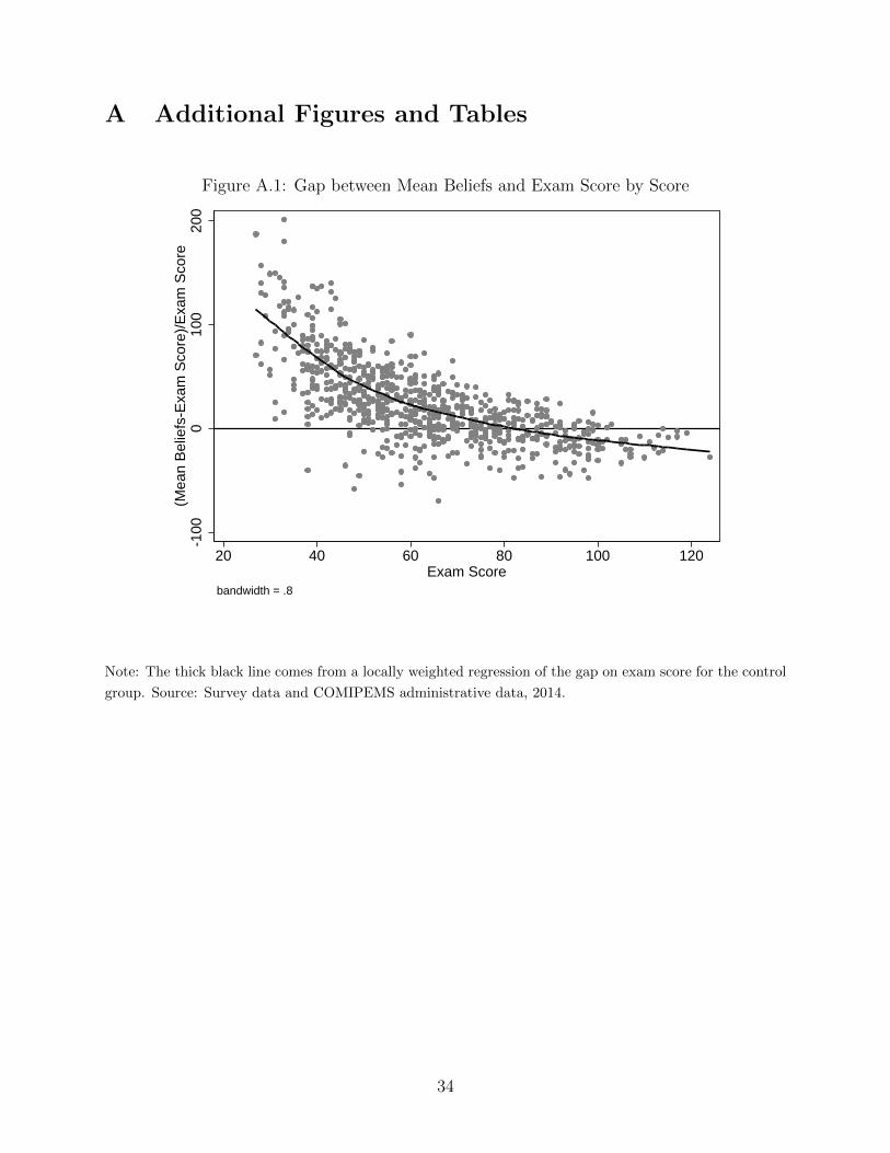
A Additional Figures and Tables

Figure A.1: Gap between Mean Beliefs and Exam Score by Score-1

000

100

200

(Mea

n B

elie

fs-E

xam

Sco

re)/

Exa

m S

core

20 40 60 80 100 120Exam Score

bandwidth = .8

Note: The thick black line comes from a locally weighted regression of the gap on exam score for the control

group. Source: Survey data and COMIPEMS administrative data, 2014.

34

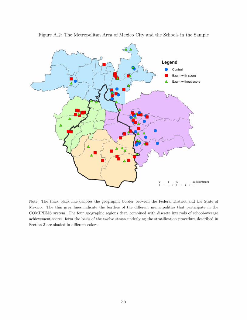
Figure A.2: The Metropolitan Area of Mexico City and the Schools in the Sample

#*

#*")

#*

#*

")")

#*

!(

")

!(

#*

")#*

")")

")

")

#*

#*

")

#*

#*

#* ")

")

#*")

")

#*#*#*

")

")

")

#*

")

#*

#*

#*

!(!(

")

#*

#*

!(

#*

!(

")")")

!(

#*

")#*#*

#*

!(

")

!(

")

")

#*!(

")

")

!(!( #*

")

#*

#*

!(

")

")

#*

!(

")

")

!(#*!(

#*

!(

!(

!(#*

#*!(

")

")

!(

#*

!(

#*

")

#*

")

")")

!(")

")!(

!(

#*

!(#*

")

")

#*

#*

#*

!(

#*

")

!(

#*

0 10 205 Kilometers

Legend!( Control") Exam with score#* Exam without score

Note: The thick black line denotes the geographic border between the Federal District and the State of

Mexico. The thin grey lines indicate the borders of the different municipalities that participate in the

COMIPEMS system. The four geographic regions that, combined with discrete intervals of school-average

achievement scores, form the basis of the twelve strata underlying the stratification procedure described in

Section 3 are shaded in different colors.

35

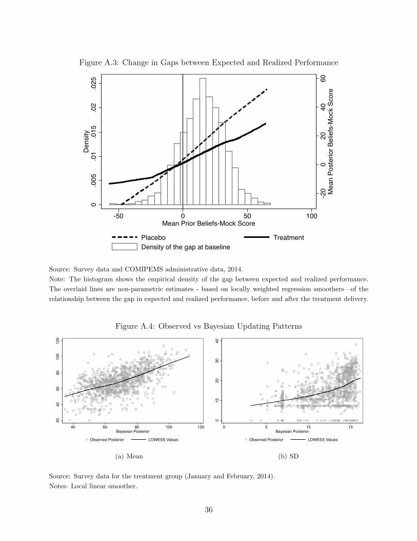
Figure A.3: Change in Gaps between Expected and Realized Performance

-20

020

4060

Mea

n Po

ster

ior B

elie

fs-M

ock

Scor

e

0.0

05.0

1.0

15.0

2.0

25D

ensi

ty

-50 0 50 100Mean Prior Beliefs-Mock Score

Placebo TreatmentDensity of the gap at baseline

Source: Survey data and COMIPEMS administrative data, 2014.

Note: The histogram shows the empirical density of the gap between expected and realized performance.

The overlaid lines are non-parametric estimates - based on locally weighted regression smoothers—of the

relationship between the gap in expected and realized performance, before and after the treatment delivery.

Figure A.4: Observed vs Bayesian Updating Patterns

2040

6080

100

120

40 60 80 100 120Bayesian Posterior

Observed Posterior LOWESS Values

(a) Mean

010

2030

40

0 5 10 15Bayesian Posterior

Observed Posterior LOWESS Values

(b) SD

Source: Survey data for the treatment group (January and February, 2014).

Notes: Local linear smoother.

36

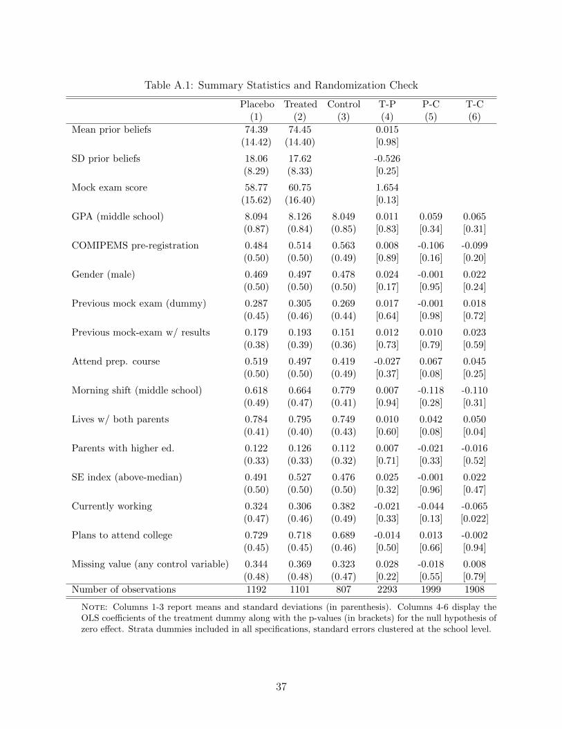
Table A.1: Summary Statistics and Randomization Check

Placebo Treated Control T-P P-C T-C(1) (2) (3) (4) (5) (6)

Mean prior beliefs 74.39 74.45 0.015(14.42) (14.40) [0.98]

SD prior beliefs 18.06 17.62 -0.526(8.29) (8.33) [0.25]

Mock exam score 58.77 60.75 1.654(15.62) (16.40) [0.13]

GPA (middle school) 8.094 8.126 8.049 0.011 0.059 0.065(0.87) (0.84) (0.85) [0.83] [0.34] [0.31]

COMIPEMS pre-registration 0.484 0.514 0.563 0.008 -0.106 -0.099(0.50) (0.50) (0.49) [0.89] [0.16] [0.20]

Gender (male) 0.469 0.497 0.478 0.024 -0.001 0.022(0.50) (0.50) (0.50) [0.17] [0.95] [0.24]

Previous mock exam (dummy) 0.287 0.305 0.269 0.017 -0.001 0.018(0.45) (0.46) (0.44) [0.64] [0.98] [0.72]

Previous mock-exam w/ results 0.179 0.193 0.151 0.012 0.010 0.023(0.38) (0.39) (0.36) [0.73] [0.79] [0.59]

Attend prep. course 0.519 0.497 0.419 -0.027 0.067 0.045(0.50) (0.50) (0.49) [0.37] [0.08] [0.25]

Morning shift (middle school) 0.618 0.664 0.779 0.007 -0.118 -0.110(0.49) (0.47) (0.41) [0.94] [0.28] [0.31]

Lives w/ both parents 0.784 0.795 0.749 0.010 0.042 0.050(0.41) (0.40) (0.43) [0.60] [0.08] [0.04]

Parents with higher ed. 0.122 0.126 0.112 0.007 -0.021 -0.016(0.33) (0.33) (0.32) [0.71] [0.33] [0.52]

SE index (above-median) 0.491 0.527 0.476 0.025 -0.001 0.022(0.50) (0.50) (0.50) [0.32] [0.96] [0.47]

Currently working 0.324 0.306 0.382 -0.021 -0.044 -0.065(0.47) (0.46) (0.49) [0.33] [0.13] [0.022]

Plans to attend college 0.729 0.718 0.689 -0.014 0.013 -0.002(0.45) (0.45) (0.46) [0.50] [0.66] [0.94]

Missing value (any control variable) 0.344 0.369 0.323 0.028 -0.018 0.008(0.48) (0.48) (0.47) [0.22] [0.55] [0.79]

Number of observations 1192 1101 807 2293 1999 1908

Note: Columns 1-3 report means and standard deviations (in parenthesis). Columns 4-6 display theOLS coefficients of the treatment dummy along with the p-values (in brackets) for the null hypothesis ofzero effect. Strata dummies included in all specifications, standard errors clustered at the school level.

37

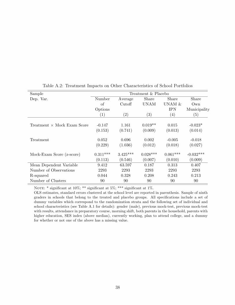
Table A.2: Treatment Impacts on Other Characteristics of School Portfolios

Sample Treatment & PlaceboDep. Var. Number Average Share Share Share

of Cutoff UNAM UNAM & OwnOptions IPN Municipality

(1) (2) (3) (4) (5)

Treatment × Mock Exam Score -0.147 1.161 0.019** 0.015 -0.023*(0.153) (0.741) (0.009) (0.013) (0.014)

Treatment 0.052 0.696 0.002 -0.005 -0.018(0.229) (1.036) (0.012) (0.018) (0.027)

Mock-Exam Score (z-score) 0.311*** 3.425*** 0.028*** 0.061*** -0.032***(0.113) (0.546) (0.007) (0.010) (0.009)

Mean Dependent Variable 9.412 63.597 0.187 0.313 0.407Number of Observations 2293 2293 2293 2293 2293R-squared 0.044 0.328 0.208 0.243 0.213Number of Clusters 90 90 90 90 90

Note: * significant at 10%; ** significant at 5%; *** significant at 1%.OLS estimates, standard errors clustered at the school level are reported in parenthesis. Sample of ninthgraders in schools that belong to the treated and placebo groups. All specifications include a set ofdummy variables which correspond to the randomization strata and the following set of individual andschool characteristics (see Table A.1 for details): gender (male), previous mock-test, previous mock-testwith results, attendance in preparatory course, morning shift, both parents in the household, parents withhigher education, SES index (above median), currently working, plan to attend college, and a dummyfor whether or not one of the above has a missing value.

38

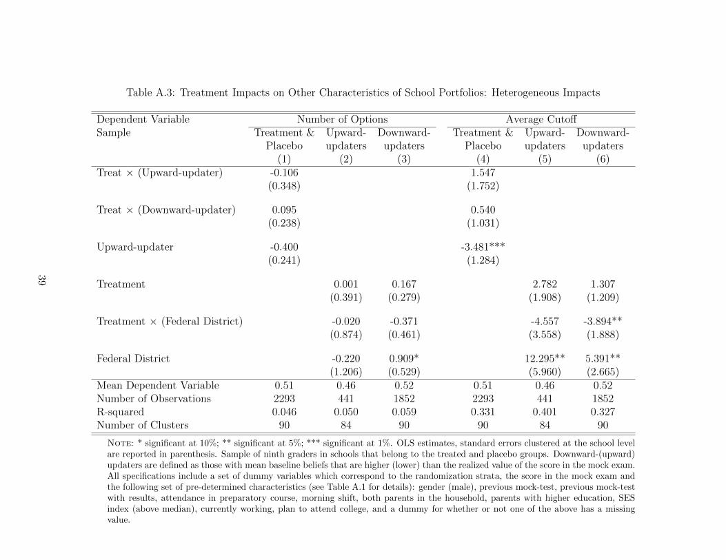
Table A.3: Treatment Impacts on Other Characteristics of School Portfolios: Heterogeneous Impacts

Dependent Variable Number of Options Average CutoffSample Treatment & Upward- Downward- Treatment & Upward- Downward-

Placebo updaters updaters Placebo updaters updaters(1) (2) (3) (4) (5) (6)

Treat × (Upward-updater) -0.106 1.547(0.348) (1.752)

Treat × (Downward-updater) 0.095 0.540(0.238) (1.031)

Upward-updater -0.400 -3.481***(0.241) (1.284)

Treatment 0.001 0.167 2.782 1.307(0.391) (0.279) (1.908) (1.209)

Treatment × (Federal District) -0.020 -0.371 -4.557 -3.894**(0.874) (0.461) (3.558) (1.888)

Federal District -0.220 0.909* 12.295** 5.391**(1.206) (0.529) (5.960) (2.665)

Mean Dependent Variable 0.51 0.46 0.52 0.51 0.46 0.52Number of Observations 2293 441 1852 2293 441 1852R-squared 0.046 0.050 0.059 0.331 0.401 0.327Number of Clusters 90 84 90 90 84 90

Note: * significant at 10%; ** significant at 5%; *** significant at 1%. OLS estimates, standard errors clustered at the school levelare reported in parenthesis. Sample of ninth graders in schools that belong to the treated and placebo groups. Downward-(upward)updaters are defined as those with mean baseline beliefs that are higher (lower) than the realized value of the score in the mock exam.All specifications include a set of dummy variables which correspond to the randomization strata, the score in the mock exam andthe following set of pre-determined characteristics (see Table A.1 for details): gender (male), previous mock-test, previous mock-testwith results, attendance in preparatory course, morning shift, both parents in the household, parents with higher education, SESindex (above median), currently working, plan to attend college, and a dummy for whether or not one of the above has a missingvalue.

39

B Relative Vs. Absolute Updating

Using the information from the socio-demographic survey completed upon registration, wecan measure students’ self-perceptions about their relative standing in the classroom in fourcourses: Math, Spanish, History, and Biology. These four variables are given values of -1,0, and 1 depending on the student classifying himself as below, as good as, and above otherstudents in the classroom. We construct a composite measure of initial relative ranking andsum up over these variables to classify students into three groups of initial relative beliefs.If the sum is negative, students are assumed to have individual beliefs below the expectedclassroom mean whereas those with positive sums are assumed to have individual beliefsabove their classroom mean. We can then compare these initial relative beliefs to eachapplicant’s actual ranking in the classroom based on their performance in the mock exam,and identify the group of right-updaters and left-updaters in terms of relative beliefs.39

According to this definition, 16 percent of the applicants in the placebo group are clas-sified as right-updaters. Among those, only 31 percent are also classified as right-updatersin terms of their individual beliefs, indicating the presence of substantial discrepancies be-tween the two definitions. Table B.1 presents the results from OLS regressions similar tothe ones reported in columns 1 and 2 in Table 2 but now we add indicator variables forrelative updating behaviors as well as their interaction terms with the treatment variable(the excluded category is the no relative update status).40 The estimates reveal the presenceof some updating in relative terms, notably for those who reported themselves as betterthan the average in their class. However, the main treatment impacts through changes inperceptions about own performance in the test in absolute terms are very similar to the onesreported in columns 1 and 2 in Table 2, in both magnitude and precision. This evidencesuggests that updating in absolute terms induces a direct change in the individual beliefdistribution far and beyond the indirect effect that changes in relative beliefs may have.

39More precisely, those variables are constructed as follows. Students with positive (negative) relativebeliefs whose mock exam score is either between 5 points above and 5 points below the average in theclassroom or 5 points below (above) the average are assumed to be more likely to update downward (upward)in terms of their relative ranking. Students with expected relative rankings that are consistent with theirranking in the distribution of the mock exam score in the classroom are considered to be non-updaters.

40We lose 162 observations (7% of the sample) due to missing values in the students’ self-perceptionsvariable collected in the registration survey. As expected though, the treatment is orthogonal to the resultingcensoring in the estimation sample.

40

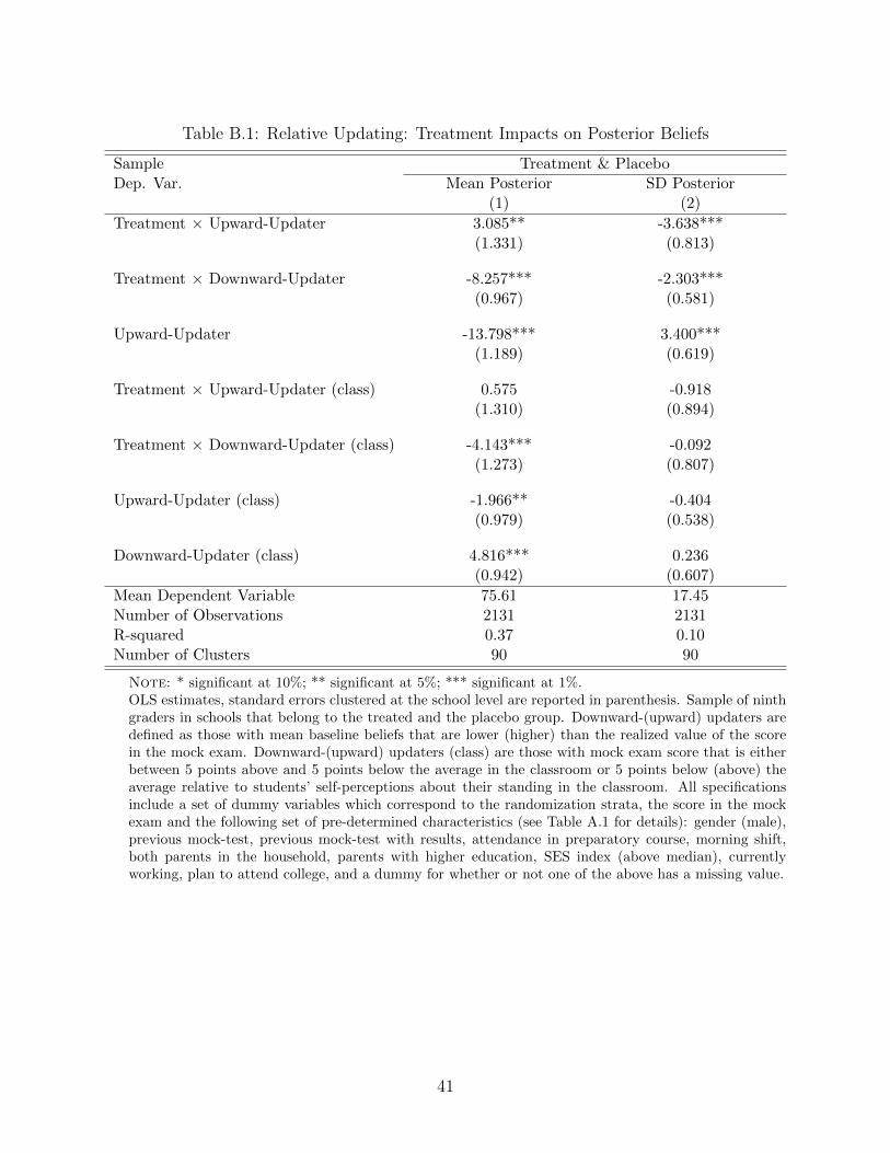
Table B.1: Relative Updating: Treatment Impacts on Posterior Beliefs

Sample Treatment & PlaceboDep. Var. Mean Posterior SD Posterior

(1) (2)

Treatment × Upward-Updater 3.085** -3.638***(1.331) (0.813)

Treatment × Downward-Updater -8.257*** -2.303***(0.967) (0.581)

Upward-Updater -13.798*** 3.400***(1.189) (0.619)

Treatment × Upward-Updater (class) 0.575 -0.918(1.310) (0.894)

Treatment × Downward-Updater (class) -4.143*** -0.092(1.273) (0.807)

Upward-Updater (class) -1.966** -0.404(0.979) (0.538)

Downward-Updater (class) 4.816*** 0.236(0.942) (0.607)

Mean Dependent Variable 75.61 17.45Number of Observations 2131 2131R-squared 0.37 0.10Number of Clusters 90 90

Note: * significant at 10%; ** significant at 5%; *** significant at 1%.OLS estimates, standard errors clustered at the school level are reported in parenthesis. Sample of ninthgraders in schools that belong to the treated and the placebo group. Downward-(upward) updaters aredefined as those with mean baseline beliefs that are lower (higher) than the realized value of the scorein the mock exam. Downward-(upward) updaters (class) are those with mock exam score that is eitherbetween 5 points above and 5 points below the average in the classroom or 5 points below (above) theaverage relative to students’ self-perceptions about their standing in the classroom. All specificationsinclude a set of dummy variables which correspond to the randomization strata, the score in the mockexam and the following set of pre-determined characteristics (see Table A.1 for details): gender (male),previous mock-test, previous mock-test with results, attendance in preparatory course, morning shift,both parents in the household, parents with higher education, SES index (above median), currentlyworking, plan to attend college, and a dummy for whether or not one of the above has a missing value.

41

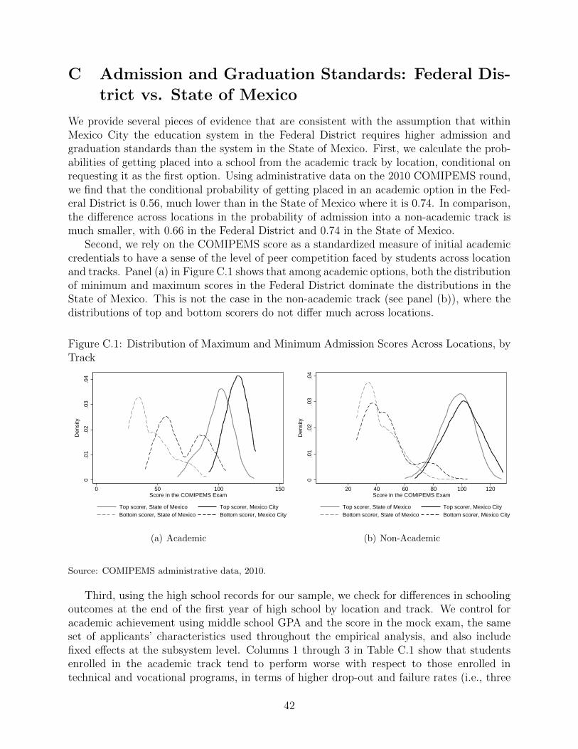
C Admission and Graduation Standards: Federal Dis-

trict vs. State of Mexico

We provide several pieces of evidence that are consistent with the assumption that withinMexico City the education system in the Federal District requires higher admission andgraduation standards than the system in the State of Mexico. First, we calculate the prob-abilities of getting placed into a school from the academic track by location, conditional onrequesting it as the first option. Using administrative data on the 2010 COMIPEMS round,we find that the conditional probability of getting placed in an academic option in the Fed-eral District is 0.56, much lower than in the State of Mexico where it is 0.74. In comparison,the difference across locations in the probability of admission into a non-academic track ismuch smaller, with 0.66 in the Federal District and 0.74 in the State of Mexico.

Second, we rely on the COMIPEMS score as a standardized measure of initial academiccredentials to have a sense of the level of peer competition faced by students across locationand tracks. Panel (a) in Figure C.1 shows that among academic options, both the distributionof minimum and maximum scores in the Federal District dominate the distributions in theState of Mexico. This is not the case in the non-academic track (see panel (b)), where thedistributions of top and bottom scorers do not differ much across locations.

Figure C.1: Distribution of Maximum and Minimum Admission Scores Across Locations, byTrack

0.0

1.0

2.0

3.0

4

Den

sity

0 50 100 150Score in the COMIPEMS Exam

Top scorer, State of Mexico Top scorer, Mexico CityBottom scorer, State of Mexico Bottom scorer, Mexico City

(a) Academic

0.0

1.0

2.0

3.0

4

Den

sity

20 40 60 80 100 120Score in the COMIPEMS Exam

Top scorer, State of Mexico Top scorer, Mexico CityBottom scorer, State of Mexico Bottom scorer, Mexico City

(b) Non-Academic

Source: COMIPEMS administrative data, 2010.

Third, using the high school records for our sample, we check for differences in schoolingoutcomes at the end of the first year of high school by location and track. We control foracademic achievement using middle school GPA and the score in the mock exam, the sameset of applicants’ characteristics used throughout the empirical analysis, and also includefixed effects at the subsystem level. Columns 1 through 3 in Table C.1 show that studentsenrolled in the academic track tend to perform worse with respect to those enrolled intechnical and vocational programs, in terms of higher drop-out and failure rates (i.e., three

42

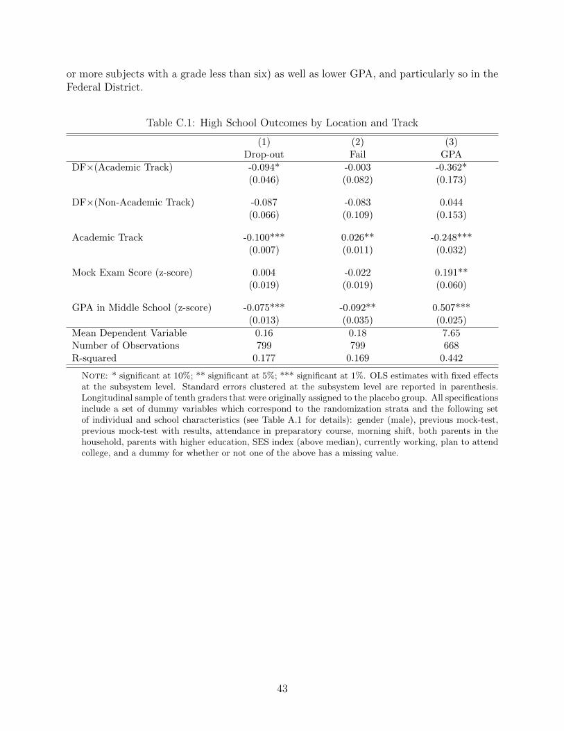
or more subjects with a grade less than six) as well as lower GPA, and particularly so in theFederal District.

Table C.1: High School Outcomes by Location and Track

(1) (2) (3)Drop-out Fail GPA

DF×(Academic Track) -0.094* -0.003 -0.362*(0.046) (0.082) (0.173)

DF×(Non-Academic Track) -0.087 -0.083 0.044(0.066) (0.109) (0.153)

Academic Track -0.100*** 0.026** -0.248***(0.007) (0.011) (0.032)

Mock Exam Score (z-score) 0.004 -0.022 0.191**(0.019) (0.019) (0.060)

GPA in Middle School (z-score) -0.075*** -0.092** 0.507***(0.013) (0.035) (0.025)

Mean Dependent Variable 0.16 0.18 7.65Number of Observations 799 799 668R-squared 0.177 0.169 0.442

Note: * significant at 10%; ** significant at 5%; *** significant at 1%. OLS estimates with fixed effectsat the subsystem level. Standard errors clustered at the subsystem level are reported in parenthesis.Longitudinal sample of tenth graders that were originally assigned to the placebo group. All specificationsinclude a set of dummy variables which correspond to the randomization strata and the following setof individual and school characteristics (see Table A.1 for details): gender (male), previous mock-test,previous mock-test with results, attendance in preparatory course, morning shift, both parents in thehousehold, parents with higher education, SES index (above median), currently working, plan to attendcollege, and a dummy for whether or not one of the above has a missing value.

43