Learning Aggregate Functions with Neural Networks Using a - Lirias

Learning Aggregate Functions with NeuralNetworks Using a Cascade-Correlation Approach

Werner Uwents1 and Hendrik Blockeel1,2

1 Department of Computer Science, Katholieke Universiteit Leuven2 Leiden Institute of Advanced Computer Science, Leiden University

Abstract. In various application domains, data can be represented asbags of vectors. Learning functions over such bags is a challenging problem.In this paper, a neural network approach, based on cascade-correlationnetworks, is proposed to handle this kind of data. By defining special ag-gregation units that are integrated in the network, a general framework tolearn functions over bags is obtained. Results on both artificially createdand real-world data sets are reported.

1 Introduction and Context

In general, two types of approaches to relational data mining can be distin-guished. In the first type, the propositionalization approach, each data elementis summarized into a vector of fixed length. We will refer to the components ofthis vector as features. In the second type, the direct approach, no summariza-tion is performed and structured data elements are handled directly. A searchis performed through a large hypothesis space, which may contain for instance(sets of) logical clauses.

The hypotheses searched by a relational learner could themselves be consid-ered features of the data, i.e., the search for a suitable hypothesis can be seen asa search in a feature space. For instance, in the context of ILP, typically the finalmodel built is a set of clauses, where the clauses are learned one by one. Thesingle clauses could be said to be boolean features, combined into a disjunction.

From this point of view, propositionalization approaches are in principle equallypowerful as direct approaches. In practice, including a separate feature for eachclause in the search space in the fixed-size vector is often not feasible because thefeature space is too large and might even be infinite. Direct approaches can be seenas “lazy propositionalization” approaches: they perform a greedy search throughthe feature space, gradually constructing relevant features.

If we look at the kind of features that are constructed by a relational learner,an essential property of these features is that they map sets of objects to a singlescalar value. Such functions are called aggregate functions and they play a key rolein relational learners. For instance, in ILP, if we have a clause happy father(X) :-child(Y,X), the “feature” constructed is essentially of the form ∃ y : Child(y, x),which tests if the set of all y’s related to x through the Child relation is emptyor not.

F. Zelezny and N. Lavrac (Eds.): ILP 2008, LNAI 5194, pp. 315–329, 2008.c© Springer-Verlag Berlin Heidelberg 2008

316 Werner Uwents and Hendrik Blockeel

As has been pointed out by Blockeel and Bruynooghe [1], the features con-structed by relational learning systems are generally of the form F(σC(S)) withS a set of objects, C a condition defined over single objects, σ the selection op-erator from relational algebra, and F an aggregate function, which maps a set toa scalar. In the above clause, S is the set of children of x, C is true, and F is the“there exists” operator (∃). For the clause happy father(X) :- child(Y,X),age(Y,A), A < 12, S and F are the same, but C is now a condition on the ageof the children.

Blockeel and Bruynooghe further pointed out that ILP systems typically con-struct structurally complex conditions but always use the same, trivial, aggregatefunction, namely ∃. The importance of using more complex aggregate functionshas been recognized by many people [2,3]. Most systems that handle such com-plex aggregate functions follow the propositionalization approach. The reason forthis is that the structure of the search space of features of the form F(σC(S))becomes much more complex and difficult to search when F can be somethingelse than ∃ [4]. But to keep the propositionalization approach feasible, a limitedset of F functions still needs to be used, and the number of different C consid-ered for σC must remain limited. For instance, Krogel and Wrobel [3] allow asingle attribute test in C, but no conjunctions.

Given the limitations of the propositionalization approach, it is useful to studyhow direct approaches could include aggregate functions other than ∃. More re-cently, methods for learning relevant features of the form F(σC(S)) have beenproposed. Vens, Van Assche et al. [5,6] proposed a random forest approach thatavoids the problems of searching a complex-structured search space, while Vens[4] studied the monotonicity properties of features of the form F(σC(S)) andshowed how efficient refinement of such features is possible for the most com-monly occurring aggregate functions.

In parallel, Uwents et al. studied to what extent subsymbolic concepts onrelational data can be learned using neural network approaches. Recurrent neuralnetworks were first proposed to learn the aggregate features, leading to theconcept of relational neural networks [7]. While a regular network maps oneinput vector to an output vector, recurrent networks can map a sequence ofinput vectors to a single output vector. This property was exploited to handlesets of vectors, the elements of which were input in random order in the network.

From the explanation above, it is clear that learning aggregate features fromsets is a crucial part of any relation learner. In this paper, we therefore focus onthe subsymbolic learning of aggregate functions as such, without considering thepossibility of having many different relationships. This means that the generalrelational learning setting is restricted to the situation where there is just asingle one-to-many relationship. This relationship results in bags of vectors withassociated target vectors. This resembles the multi-instance setting, because inmulti-instance learning, one also deals with data sets containing a bag of vectorsfor each data instance. However, in multi-instance learning the hypothesis thatshould be learned has some restrictions. Each bag is classified as positive ornegative but this classification can be reformulated in terms of a classification

Learning Aggregate Functions with Neural Networks 317

of the individual vectors in the bag. If all vectors are negative, the bag as awhole will also be classified as negative. If there is at least one positive vector,the bag will be classified as positive. Learning aggregate functions in general ismore complicated because these restrictions do no longer apply and the classof possible aggregate functions is very broad and diverse. In this paper, we willconsider the use of neural networks for learning this kind of general aggregatefunctions. For the multi-instance setting, the use of neural networks has beenexplored before by Ramon and De Raedt [9]. They make use of a softmax functionin the network, similar to what will be used in our aggregate cascade-correlationnetworks as explained in section 2.2.

The remainder of the paper is structured as follows. In section 2 we reviewcascade-correlation networks and we adapt these networks so that they can rep-resent aggregation functions, this by introducing a limited number of aggregationunits in them. A training procedure for such networks is also described. In section3 we experimentally evaluate the method, to conclude in section 4.

2 Aggregate Cascade-Correlation Networks

Cascade-correlation networks are a special kind of neural networks, constructedone unit at a time. In the next subsection, the original cascade-correlation al-gorithm will be discussed. After that, a number of new units, capable of ag-gregating, will be presented. These units will then be integrated in an adaptedversion of cascade-correlation, resulting in a network structure that can learnconcepts with aggregation. The resulting networks are called aggregate cascade-correlation networks (ACCNs).

2.1 The Original Cascade-Correlation Network

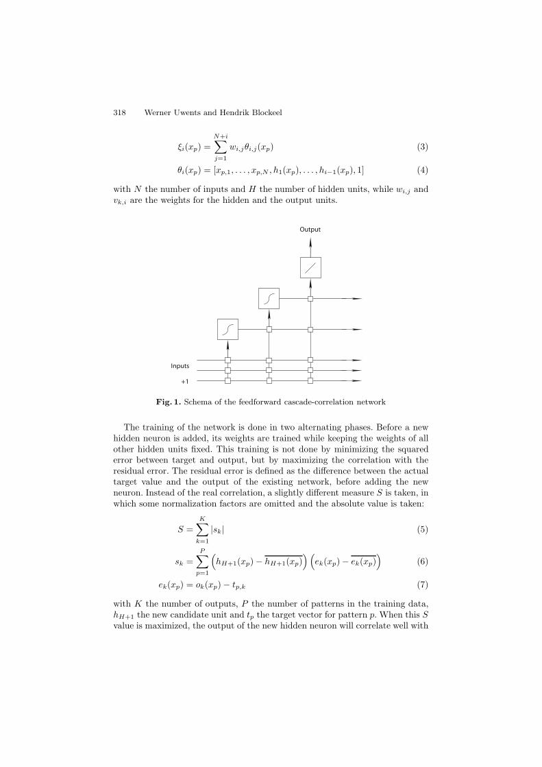
The idea behind the original cascade-correlation algorithm [10] is to learn notonly the weights, but also the structure of the network at the same time. This isdone in a constructive way, meaning that only one neuron at a time is trained andthen added to the network. One starts with a network without any hidden unit,and then hidden neurons are added, one by one, until some stopping criterionis satisfied. Once a hidden neuron has been added to the network, its weightsremain fixed throughout the rest of the procedure. This also means that, besidesthe actual input vector, the output values of these existing hidden units can beused as extra inputs for any new hidden neuron. At the output, a linear functioncan be used. A schema of the network is shown in figure 1. For an input vectorxp, the output values op,k of the network are then computed as

ok(xp) =N∑

i=1

vk,ixp,i +H∑

i=1

vk,ihi(xp) + vk,N+H+1 (1)

hi(xp) = σ(ξi(xp)) (2)


ξi(xp) =N+i∑

j=1

wi,jθi,j(xp) (3)

θi(xp) = [xp,1, . . . , xp,N , h1(xp), . . . , hi−1(xp), 1] (4)

with N the number of inputs and H the number of hidden units, while wi,j andvk,i are the weights for the hidden and the output units.

Inputs

+1

Output

Fig. 1. Schema of the feedforward cascade-correlation network

The training of the network is done in two alternating phases. Before a newhidden neuron is added, its weights are trained while keeping the weights of allother hidden units fixed. This training is not done by minimizing the squarederror between target and output, but by maximizing the correlation with theresidual error. The residual error is defined as the difference between the actualtarget value and the output of the existing network, before adding the newneuron. Instead of the real correlation, a slightly different measure S is taken, inwhich some normalization factors are omitted and the absolute value is taken:

S =K∑

k=1

|sk| (5)

sk =P∑

p=1

(hH+1(xp) − hH+1(xp)

) (ek(xp) − ek(xp)

)(6)

ek(xp) = ok(xp) − tp,k (7)

with K the number of outputs, P the number of patterns in the training data,hH+1 the new candidate unit and tp the target vector for pattern p. When this Svalue is maximized, the output of the new hidden neuron will correlate well with


the residual error. The key idea here is that a unit that correlates well with theresidual error, will help to reduce the output error when added to the network.The maximization is done by computing the gradient and performing some formof gradient descent. This gradient is computed as follows:

∂S

∂wi=

K∑

k=1

P∑

p=1

sign(sk)σ′(ξH+1(xp)) (ek(xp) − ek(xp)) θH+1,i(xp) (8)

Instead of training only one candidate neuron at a time, a pool of neurons,initialized with random weights, can be trained. At the end, the best one isselected. This increases the chance that a good candidate will be found. Oncethe best candidate is selected and added to the network, the output weights forthe updated network can be trained. If a linear function is used at the outputs,the output weights can be obtained by simple linear regression.

2.2 Cascade-Correlation with Aggregation Units

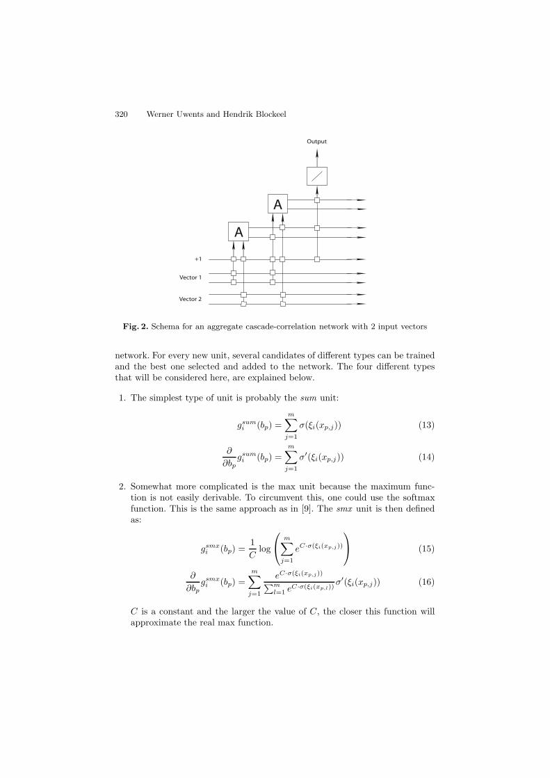
The concept of cascade-correlation networks can be extended to networks forlearning aggregate functions. The crucial difference is that instead of the simplehidden neurons, units that can process bags are used. For the rest, the networkand the training of it works in the same way as for the feedforward networks. Thedata set now consists of bags bp = {xp,1, . . . , xp,m}, where xp,i are vectors of sizeN , with associated target vectors tp. Because the input is a bag of vectors insteadof one single vector, it can no longer be used as direct input for the output units,and so this is dropped from the equation. Each input bag bp = {xp,1, . . . , xp,m}of a pattern p will be processed by the hidden units. Each time a vector of thebags has been processed, an intermediate output value for the hidden units canbe computed, yielding a sequence of m values for each hidden unit. The finalvalue is used by the output units, but the whole sequence of values can also beused by new hidden units. A schema of an aggregate cascade-correlation networkfor 2 input vectors is shown in figure 2. The network then becomes:

ok(bp) =H∑

i=1

vk,ihi,m(bp) + vk,H+1 (9)

hi,j(bp) = gi({ξi(xp,1), . . . , ξi(xp,j)}) (10)

ξi(xp,j) =N+i∑

l=1

wi,lθi,l(xp,j) (11)

θi(xp,j) = [xp,1, . . . , xp,N , h1,j(xp), . . . , hi−1,j(xp), 1] (12)

with gi a special function. Different functions can be used for gi, as long asthey perform some kind of aggregation. One could take the sum or the maxfunction for instance. Another possibility is to use a locally recurrent neuron.The only condition imposed on the gi function is that it must be derivable toallow gradient training. Different types of units can easily be combined in the


Vector 1

+1

Output

A

A

Vector 2

Fig. 2. Schema for an aggregate cascade-correlation network with 2 input vectors

network. For every new unit, several candidates of different types can be trainedand the best one selected and added to the network. The four different typesthat will be considered here, are explained below.

1. The simplest type of unit is probably the sum unit:

gsumi (bp) =

m∑

j=1

σ(ξi(xp,j)) (13)

∂

∂bpgsum

i (bp) =m∑

j=1

σ′(ξi(xp,j)) (14)

2. Somewhat more complicated is the max unit because the maximum func-tion is not easily derivable. To circumvent this, one could use the softmaxfunction. This is the same approach as in [9]. The smx unit is then definedas:

gsmxi (bp) =

1C

log

⎛

⎝m∑

j=1

eC·σ(ξi(xp,j))

⎞

⎠ (15)

∂

∂bpgsmx

i (bp) =m∑

j=1

eC·σ(ξi(xp,j))∑m

l=1 eC·σ(ξi(xp,l))σ′(ξi(xp,j)) (16)

C is a constant and the larger the value of C, the closer this function willapproximate the real max function.


3. Instead of choosing a value for C that is large enough to give a good approx-imation, one could take the limit for C going to infinity, which gives the realmax function and its derivative:

max{x1, . . . , xn} = limC→∞

1C

n∑

i=1

eC·xi (17)

∂

∂xjmax{x1, . . . , xn} =

{1 if xj = max{x1, . . . , xn}0 otherwise

(18)

A possible disadvantage with this exact function is that the derivative is notcontinuous anymore, which can deteriorate learning. The corresponding maxunit then becomes:

gmaxi (bp) = max({σ(ξi(xp,1)), . . . , σ(ξi(xp,k))}) (19)

∂

∂bpgsmx

i (bp) = σ′(ξi(xp,l∗)) with σ(ξi(xp,l∗)) = gmaxi (bp) (20)

4. The fourth type of unit considered here, is the locally recurrent unit. This isa standard feedforward unit with one recurrent connection with itself added.This lrc unit is defined as:

glrci (bp) = σ(ξi(xp,k) + wrg

lrci (bp\{xp,k})) (21)

Gradient computation for this type of unit is done using backpropagationthrough time [11].

New types of units could easily be invented if necessary, but only these fourwill be considered in the rest of the paper.

2.3 Aggregate Cascade-Correlation Training

With all parts of the aggregate cascade-correlation network explained, it onlyremains to discuss the training of the network in more detail. Each time a newunit should be added to the hidden layer, a pool of units is created of the fourtypes discussed in the previous subsection. Weights are initialized randomly.After that, all units in the pool are trained for a number of iterations, similarto backpropagation. This training is basically a gradient ascent, maximizing thecorrelation with the outputs as given in formula 5. The computation of thegradient depends of course on the type of unit. The gradient ascent itself isactually done by using resilient propagation, as described in [12]. This methodhas the advantage that the step size is determined automatically and convergenceis faster than for a fixed step size. The basic idea is to increase the step size whenthe sign of the gradient remains the same, and decrease the step size when thesign changes.

When all units in the pool have been trained, the best one is chosen. Inthis case, the best unit is the one with the highest correlation. To be able to


compare units of different types with each other, the absolute value of the realcorrelation has to be computed, and not the S-value from formula 5 in whichsome normalization constants were omitted. When the unit with the highestcorrelation has been chosen, it is installed in the network and the output weightshave to be learned again. Because linear activation functions are used for theoutput units, the output weights can be determined with least squares linearregression.

In the ideal case, when there is enough data available, a validation set canbe used to determine when to stop adding new units. If this is difficult, thereis also an alternative stopping criterion. Typically, the first units added to thenetwork will have a high correlation. When more units are added, the correlationwill decrease until no more reduction can be made. One can stop training whenthe correlation is below a certain threshold or does not decrease significantlyanymore.

3 Experiments

In this section, a number of experimental results will be discussed. First, a seriesof experiments is carried out on artificially created data sets. After that, themethod is evaluated on some real-world data sets.

3.1 Simple Aggregates

A simple experiment to examine the capacity of the aggregate cascade-correlationnetwork, is to create artificial data with predefined aggregate functions and trainthe networks on it. The data consists of bags with a variable number of elements.Each element of the bag is a vector with five components. Only the first or the firstand second component are relevant for the target value, depending on the aggre-gate function under consideration. The values of these components are randomlygenerated, but in such a way that the target values are uniformly distributed overthe possible target values. All the other components are filled with uniformly dis-tributed random numbers from the interval [−1, 1]. It is very likely that he num-ber of vectors in the bags influences the difficulty of the learning task, so differentsizes are tested. The data sets denoted as small contain 5 to 10 vectors per bag,the medium data sets 20 to 30 and the large ones 50 to 100. Each data set con-tains 3000 bags. A range of different aggregate functions are used to construct thedata sets:

1. count: the target is the number of vectors in the bag.2. sum: the target is the sum of all values of the first component of the bag

vectors.3. max: the target is the maximum value of the first component of the bag

vectors.4. avg: the target is the average value of the first component of the bag vectors.5. stddev: the target is the standard deviation of the values of the first com-

ponent of the bag vectors.


6. cmpcount: the target is the number of bag vectors for which the value ofthe first component is smaller than the value of the second component.

7. corr: the target is the correlation between the first two components of thebag vectors.

8. even: the target is one if the number of positive values for the first compo-nent is even, and zero if it is odd.

9. distr: the target is one if the values of the first component come from aGaussian distribution, and zero if they are from a uniform distribution.

10. select: the target is one if at least one of the values of the first componentlies in a given interval, and zero otherwise.

11. conj: the target is one if there is at least one vector in the bag for which thethe first and the second component lie in a certain interval.

12. disj: the target is one if there is at least one vector in the bag for which thefirst or the second component lies in a certain interval.

The first 7 data sets have a numerical target, the others a nominal target.In case of a nominal target, the number of positive and negative examples areequal. The experiments are done using 10-fold cross-validation. One fold is usedas test set, 7 folds are used for training and 2 folds are used as validation setto determine when to stop adding units. The maximum number of hidden unitsis limited to 10. The number of candidate units trained in every step is 20,which means that there are five units of every type. Each unit is trained for500 iterations, which should be more than enough to have converged to optimalweights. For the data sets with nominal target, the accuracy is reported andfor the sets with numerical targets the mean squared error is given. Standarddeviation is reported as well. The results are summarized in table 1.

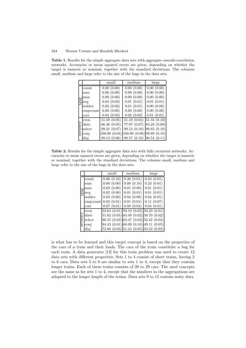
From the results, it is clear that most functions can be learned very well. Onlythe even function is really impossible to learn it seems. For the distr function,the number of vectors must be large to be able to learn it well. This makes sensebecause it is easier to say whether a bag of values comes from a normal or uniformdistribution if the bag is larger than when it is rather small. In table 2, results aregiven using fully recurrent networks, similar to what is used in relational neuralnetworks [7]. Compared with these results, it is clear that ACCNs perform better.One of the major problems with these recurrent networks, is the decreasingperformance on larger bags. If we look at the results for the select data sets forinstance, then the accuracy on the data set with small bags is still reasonable forthe recurrent network, although the accuracy for the ACCNs is better. But forthe data sets with larger bags, the accuracy goes down for the recurrent networkswhile it remains about the same for the ACCNs. Overall, it is clear that ACCNsare a better choice than the recurrent networks.

3.2 Trains

The trains data sets are also artificially created data sets containing a numberof trains. Every train consists of a number of cars, carrying some load. Some ofthe trains are eastbound, the others are westbound. The direction of the trains


Table 1. Results for the simple aggregate data sets with aggregate cascade-correlationnetworks. Accuracies or mean squared errors are given, depending on whether thetarget is numeric or nominal, together with the standard deviations. The columnssmall, medium and large refer to the size of the bags in the data sets.

small medium largeM

SE

count 0.00 (0.00) 0.00 (0.00) 0.00 (0.00)sum 0.00 (0.00) 0.00 (0.00) 0.00 (0.00)max 0.00 (0.00) 0.00 (0.00) 0.00 (0.00)avg 0.04 (0.03) 0.01 (0.01) 0.01 (0.01)stddev 0.02 (0.02) 0.01 (0.01) 0.00 (0.00)cmpcount 0.00 (0.00) 0.00 (0.00) 0.00 (0.00)corr 0.04 (0.03) 0.02 (0.02) 0.01 (0.01)

accu

racy

even 51.59 (0.05) 51.10 (0.04) 51.34 (0.10)distr 66.48 (0.05) 77.97 (0.07) 84.23 (0.09)select 99.21 (0.07) 99.13 (0.10) 98.83 (0.10)conj 100.00 (0.04) 100.00 (0.00) 99.89 (0.10)disj 99.13 (0.06) 98.57 (0.10) 96.54 (0.11)

Table 2. Results for the simple aggregate data sets with fully recurrent networks. Ac-curacies or mean squared errors are given, depending on whether the target is numericor nominal, together with the standard deviations. The columns small, medium andlarge refer to the size of the bags in the data sets.

small medium large

MSE

count 0.06 (0.10) 0.26 (0.01) 0.23 (0.01)sum 0.00 (0.00) 0.09 (0.10) 0.23 (0.01)max 0.02 (0.00) 0.01 (0.00) 0.01 (0.01)avg 0.02 (0.00) 0.01 (0.01) 0.01 (0.01)stddev 0.03 (0.00) 0.04 (0.00) 0.04 (0.01)cmpcount 0.02 (0.01) 0.01 (0.01) 0.11 (0.07)corr 0.07 (0.01) 0.08 (0.04) 0.04 (0.01)

accu

racy

even 52.64 (0.01) 50.19 (0.02) 50.23 (0.01)distr 51.62 (0.05) 63.49 (0.02) 58.70 (0.02)select 90.55 (0.03) 63.47 (0.03) 50.42 (0.02)conj 94.43 (0.01) 68.09 (0.10) 49.11 (0.05)disj 72.08 (0.03) 51.24 (0.05) 50.32 (0.02)

is what has to be learned and this target concept is based on the properties ofthe cars of a train and their loads. The cars of the train constitute a bag foreach train. A data generator [13] for this train problem was used to create 12data sets with different properties. Sets 1 to 4 consist of short trains, having 2to 6 cars. Data sets 5 to 8 are similar to sets 1 to 4, except that they containlonger trains. Each of these trains consists of 20 to 29 cars. The used conceptsare the same as for sets 1 to 4, except that the numbers in the aggregations areadapted to the longer length of the trains. Data sets 9 to 12 contain noisy data.


This means that a number of samples have been mislabeled. The used conceptsfor the different data sets are as follows:

1. Trains having at least one circle load are eastbound, the others are west-bound.

2. Trains having at least one circle or rectangle load and at least one car withpeaked roof or 3 wheels are eastbound, the others are westbound.

3. Trains having more than 8 wheels in total are eastbound, the others arewestbound.

4. Trains having more than 3 wheels in total and at least 2 rectangle loads andmaximum 5 cars are eastbound, the others are westbound.

5. Same concept as for set 1.6. Same concept as for set 2.7. Trains having more than 53 wheels in total are eastbound, the others are

westbound.8. Trains having more than 45 wheels in total and at least 10 rectangle loads

and maximum 27 cars are eastbound, the others are westbound.9. Same concept as for set 1, but with 5% noise.

10. Same concept as for set 1, but with 15% noise.11. Same concept as for set 3, but with 5% noise.12. Same concept as for set 3, but with 15% noise.

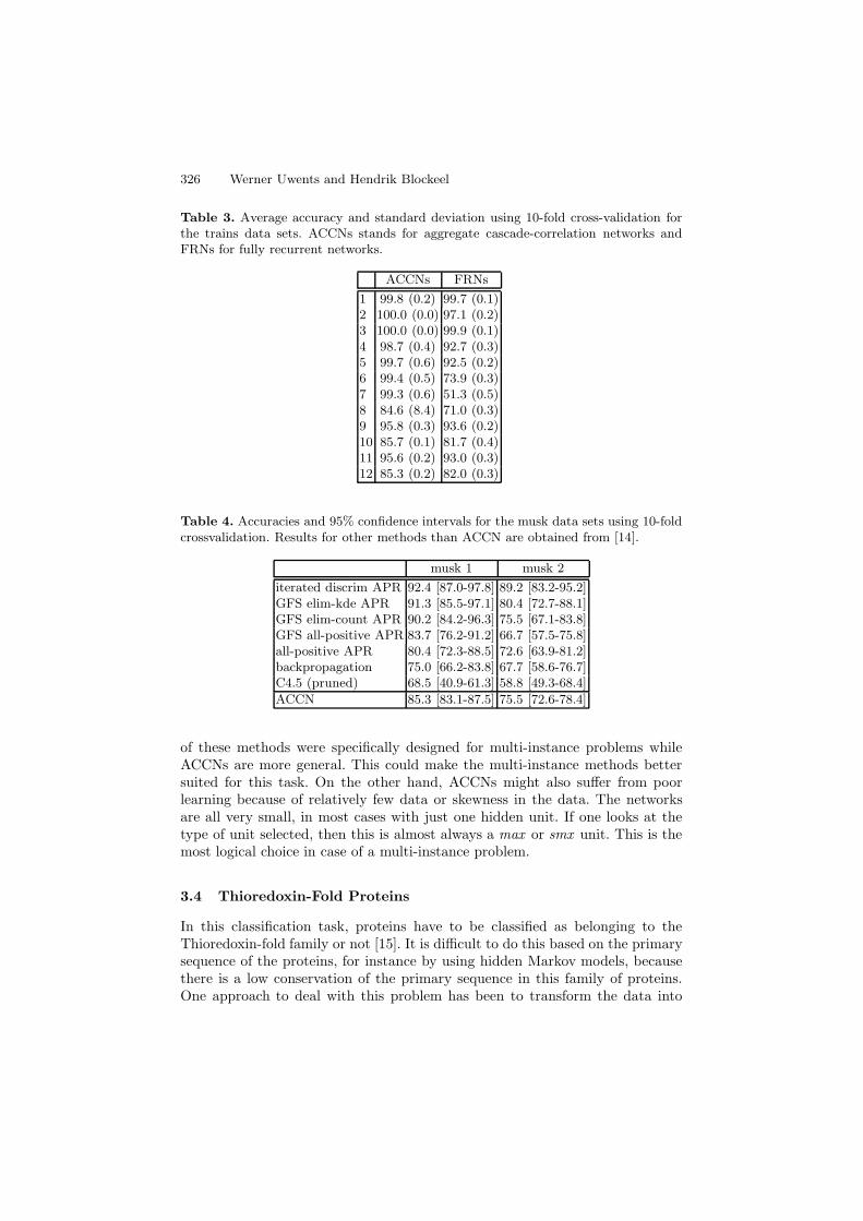
The training setup is the same as for the simple aggregate data sets. Theresults for ACCNs and fully recurrent networks are given in table 3. It is clearthat most concepts can be learned well with ACCNs. Most of the data setswithout noise have an accuracy very close to 100%. Only for set 8, which has themost difficult concept, is it impossible to get close to perfect accuracy. For thedata sets with noise, the accuracies are all close to 100% minus the percentage ofnoise, which means that the method is noise-resistant. Compared with the fullyrecurrent networks, the results for ACCNs are always better again. Sometimesthe difference is quite spectacular. Also for these data sets, the size of the bagshas an important influence on the accuracy for the recurrent networks.

3.3 Musk

Musk is a well-known multi-instance data set [14]. Each data instance stands fora molecule, represented by a bag of all its possible conformations. A conformationis described by 166 numerical features. The molecules have to be classified asmusk or non-musk. The data set consists of two parts. The first part contains92 molecules, the second part 102. In each bag, there are between 2 and 40conformations for the first part, and between 1 and 1044 for the second part.

Experiments were carried out using 10-fold cross-validation. For the ACCNs,a pool of 20 neurons and 500 training iterations are used in every step. The valueof the correlation is used as stopping criterion as described above. The resultsfor the musk data sets can be found in table 4. The accuracies for ACCNs arenot bad but not that excellent either compared with the other methods. Some


Table 3. Average accuracy and standard deviation using 10-fold cross-validation forthe trains data sets. ACCNs stands for aggregate cascade-correlation networks andFRNs for fully recurrent networks.

ACCNs FRNs1 99.8 (0.2) 99.7 (0.1)2 100.0 (0.0) 97.1 (0.2)3 100.0 (0.0) 99.9 (0.1)4 98.7 (0.4) 92.7 (0.3)5 99.7 (0.6) 92.5 (0.2)6 99.4 (0.5) 73.9 (0.3)7 99.3 (0.6) 51.3 (0.5)8 84.6 (8.4) 71.0 (0.3)9 95.8 (0.3) 93.6 (0.2)10 85.7 (0.1) 81.7 (0.4)11 95.6 (0.2) 93.0 (0.3)12 85.3 (0.2) 82.0 (0.3)

Table 4. Accuracies and 95% confidence intervals for the musk data sets using 10-foldcrossvalidation. Results for other methods than ACCN are obtained from [14].

musk 1 musk 2iterated discrim APR 92.4 [87.0-97.8] 89.2 [83.2-95.2]GFS elim-kde APR 91.3 [85.5-97.1] 80.4 [72.7-88.1]GFS elim-count APR 90.2 [84.2-96.3] 75.5 [67.1-83.8]GFS all-positive APR 83.7 [76.2-91.2] 66.7 [57.5-75.8]all-positive APR 80.4 [72.3-88.5] 72.6 [63.9-81.2]backpropagation 75.0 [66.2-83.8] 67.7 [58.6-76.7]C4.5 (pruned) 68.5 [40.9-61.3] 58.8 [49.3-68.4]ACCN 85.3 [83.1-87.5] 75.5 [72.6-78.4]

of these methods were specifically designed for multi-instance problems whileACCNs are more general. This could make the multi-instance methods bettersuited for this task. On the other hand, ACCNs might also suffer from poorlearning because of relatively few data or skewness in the data. The networksare all very small, in most cases with just one hidden unit. If one looks at thetype of unit selected, then this is almost always a max or smx unit. This is themost logical choice in case of a multi-instance problem.

3.4 Thioredoxin-Fold Proteins

In this classification task, proteins have to be classified as belonging to theThioredoxin-fold family or not [15]. It is difficult to do this based on the primarysequence of the proteins, for instance by using hidden Markov models, becausethere is a low conservation of the primary sequence in this family of proteins.One approach to deal with this problem has been to transform the data into


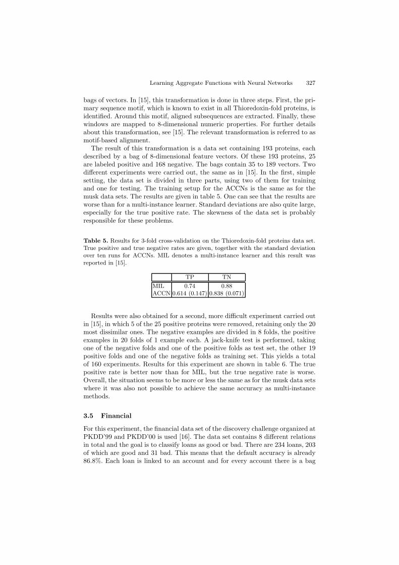
bags of vectors. In [15], this transformation is done in three steps. First, the pri-mary sequence motif, which is known to exist in all Thioredoxin-fold proteins, isidentified. Around this motif, aligned subsequences are extracted. Finally, thesewindows are mapped to 8-dimensional numeric properties. For further detailsabout this transformation, see [15]. The relevant transformation is referred to asmotif-based alignment.

The result of this transformation is a data set containing 193 proteins, eachdescribed by a bag of 8-dimensional feature vectors. Of these 193 proteins, 25are labeled positive and 168 negative. The bags contain 35 to 189 vectors. Twodifferent experiments were carried out, the same as in [15]. In the first, simplesetting, the data set is divided in three parts, using two of them for trainingand one for testing. The training setup for the ACCNs is the same as for themusk data sets. The results are given in table 5. One can see that the results areworse than for a multi-instance learner. Standard deviations are also quite large,especially for the true positive rate. The skewness of the data set is probablyresponsible for these problems.

Table 5. Results for 3-fold cross-validation on the Thioredoxin-fold proteins data set.True positive and true negative rates are given, together with the standard deviationover ten runs for ACCNs. MIL denotes a multi-instance learner and this result wasreported in [15].

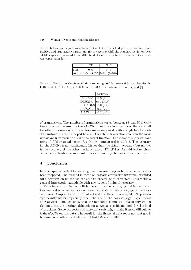
TP TNMIL 0.74 0.88ACCN 0.614 (0.147) 0.838 (0.071)

Results were also obtained for a second, more difficult experiment carried outin [15], in which 5 of the 25 positive proteins were removed, retaining only the 20most dissimilar ones. The negative examples are divided in 8 folds, the positiveexamples in 20 folds of 1 example each. A jack-knife test is performed, takingone of the negative folds and one of the positive folds as test set, the other 19positive folds and one of the negative folds as training set. This yields a totalof 160 experiments. Results for this experiment are shown in table 6. The truepositive rate is better now than for MIL, but the true negative rate is worse.Overall, the situation seems to be more or less the same as for the musk data setswhere it was also not possible to achieve the same accuracy as multi-instancemethods.

3.5 Financial

For this experiment, the financial data set of the discovery challenge organized atPKDD’99 and PKDD’00 is used [16]. The data set contains 8 different relationsin total and the goal is to classify loans as good or bad. There are 234 loans, 203of which are good and 31 bad. This means that the default accuracy is already86.8%. Each loan is linked to an account and for every account there is a bag


Table 6. Results for jack-knife tests on the Thioredoxin-fold proteins data set. Truepositive and true negative rates are given, together with the standard deviation overall 160 experiments for ACCNs. MIL stands for a multi-instance learner and this resultwas reported in [15].

TP TNMIL 0.75 0.75ACCN 0.850 (0.035) 0.681 (0.028)

Table 7. Results on the financial data set using 10-fold cross-validation. Results forFORF-LA, DINUS-C, RELAGGS and PROGOL are obtained from [17] and [3].

accuracyFORF-LA 90.8 (1.7)DINUS-C 85.1 (10.3)RELAGGS 88.0 (6.5)PROGOL 86.3 (7.1)ACCN 87.2 (2.3)

of transactions. The number of transactions varies between 93 and 594. Onlythese bags will be used by the ACCNs to learn a classification of the loans, allthe other information is ignored because we only work with a single bag for eachdata instance. It can be hoped however that these transactions contain the mostimportant information to learn the target function. The experiments were doneusing 10-fold cross-validation. Results are summarized in table 7. The accuracyfor the ACCNs is not significantly higher than the default accuracy, but neitheris the accuracy of the other methods, except FORF-LA. As said before, theseother methods also use more information than only the bags of transactions.

4 Conclusion

In this paper, a method for learning functions over bags with neural networks hasbeen proposed. The method is based on cascade-correlation networks, extendedwith aggregation units that are able to process bags of vectors. This yields ageneral framework, extendable with new types of units if necessary.

Experimental results on artificial data sets are encouraging and indicate thatthis method is indeed capable of learning a wide variety of aggregate functionsover bags. Compared with recurrent networks on these data sets, ACCNs performsignificantly better, especially when the size of the bags is large. Experimentson real-world data sets show that the method performs still reasonably well inthe multi-instance setting, although not as well as specific methods for this kindof problems. Some properties of these data sets might make it more difficult totrain ACCNs on this data. The result for the financial data set is not that good,but similar to other methods like RELAGGS and FORF.


References

1. Blockeel, H., Bruynooghe, M.: Aggregation versus selection bias, and relationalneural networks. In: Getoor, L., Jensen, D. (eds.) IJCAI 2003 Workshop on Learn-ing Statistical Models from Relational Data, SRL 2003, Acapulco, Mexico (2003)

2. Knobbe, A., Siebes, A., Marseille, B.: Involving aggregate functions in multi-relational search. In: Principles of Data Mining and Knowledge Discovery, Proceed-ings of the 6th European Conference, pp. 287–298. Springer, Heidelberg (August2002)

3. Krogel, M.A., Wrobel, S.: Transformation-based learning using multirelational ag-gregation. In: Rouveirol, C., Sebag, M. (eds.) ILP 2001. LNCS (LNAI), vol. 2157,pp. 142–155. Springer, Heidelberg (2001)

4. Vens, C., Ramon, J., Blockeel, H.: Refining aggregate conditions in relational learn-ing. In: Furnkranz, J., Scheffer, T., Spiliopoulou, M. (eds.) PKDD 2006. LNCS(LNAI), vol. 4213, pp. 383–394. Springer, Heidelberg (2006)

5. Vens, C., Van Assche, A., Blockeel, H., Dzeroski, S.: First order random forestswith complex aggregates. In: Camacho, R., King, R., Srinivasan, A. (eds.) ILP2004. LNCS (LNAI), vol. 3194, pp. 323–340. Springer, Heidelberg (2004)

6. Van Assche, A., Vens, C., Blockeel, H., Dzeroski, S.: First order random forests:Learning relational classifiers with complex aggregates. Machine Learning 64(1-3),149–182 (2006)

7. Uwents, W., Blockeel, H.: Classifying relational data with neural networks. In:Kramer, S., Pfahringer, B. (eds.) ILP 2005. LNCS (LNAI), vol. 3625, pp. 384–396.Springer, Heidelberg (2005)

8. Uwents, W., Monfardini, G., Blokeel, H., Scarsello, F., Gori, M.: Two connectionistsmodels for graph processing: An experimental comparison on relational data. In:MLG 2006, Proceedings on the International Workshop on Mining and Learningwith Graphs, pp. 211–220 (2006)

9. Ramon, J., De Raedt, L.: Multi instance neural networks. In: Raedt, L.D., Kramer,S. (eds.) Proceedings of the ICML-2000 workshop on attribute-value and relationallearning, pp. 53–60 (2000)

10. Fahlman, S.E., Lebiere, C.: The cascade-correlation learning architecture. In:Touretzky, D.S. (ed.) Advances in Neural Information Processing Systems. Denver1989, vol. 2, pp. 524–532. Morgan Kaufmann, San Mateo (1990)

11. Werbos, P.J.: Back propagation through time: What it does and how to do it.Proceedings of the IEEE 78, 1550–1560 (1990)

12. Riedmiller, M., Braun, H.: A direct adaptive method for faster backpropagationlearning: The RPROP algorithm. In: Proc. of the IEEE Intl. Conf. on NeuralNetworks, San Francisco, CA, pp. 586–591 (1993)

13. Michie, D., Muggleton, S., Page, D., Srinivasan, A.: To the international comput-ing community: A new east-west challenge. Technical report, Oxford UniversityComputing Laboratory, Oxford, UK (1994)

14. Dietterich, T.G., Lathrop, R.H., Lozano-Perez, T.: Solving the multiple instanceproblem with axis-parallel rectangles. Artificial Intelligence 89(1-2), 31–71 (1997)

15. Wang, C., Scott, S.D., Zhang, J., Tao, Q., Fomenko, D.E., Gladyshev, V.N.: Astudy in modeling low-conservation protein superfamilies. Technical Report UNL-CSE-2004-0003, University of Nebraska (2004)

16. Berka, P.: Guide to the financial data set. In: Siebes, A., Berka, P. (eds.) TheECML/PKDD 2000 Discovery Challenge (2000)

17. Vens, C.: Complex aggregates in relational learning. PhD thesis, Department ofComputer Science, KULeuven (2007)

Documents

Learning Aggregate Functions with Neural Networks Using a - Lirias