Embed Size (px)
Citation preview
Learning Ankle-Tilt and Foot-Placement Control forFlat-footed Bipedal Balancing and WalkingBernhard Hengst
Computer Science and EngineeringUniversity of New South Wales
Sydney, AustraliaEmail: [email protected]
Manuel LangeEberhard Karls University of Tubingen
Wilhelm-Schickard-Institut fur InformatikEmail: [email protected]
andComputer Science and Engineering
University of New South WalesSydney, Australia
Brock WhiteComputer Science and Engineering
University of New South WalesSydney, Australia
Email: [email protected]
Abstract—We learn a controller for a flat-footed bipedal robotto optimally respond to both (1) external disturbances causedby, for example, stepping on objects or being pushed, and (2)rapid acceleration, such as reversal of demanded walk direction.The reinforcement learning method employed learns an optimalpolicy by actuating the ankle joints to assert pressure at differentpoints along the support foot, and to determine the next swingfoot placement. The controller is learnt in simulation using aninverted pendulum model and the control policy transferred andtested on two small physical humanoid robots.
I. INTRODUCTION
Bipedal locomotion is often subjected to large impact forcesinduced by a robot inadvertently stepping on objects or bybeing pushed. In robotic soccer, for example, it is not uncom-mon for robots to step on each other’s feet or to be jostledby opposition players. At current RoboCup [1] competitionsrobots regularly fall over for these reasons in both humanoidand standard platform league matches. Another requirementin soccer environments is that bipedal robots should be ableto react optimally to rapidly changing directional goals. Insoccer it is often necessary to stop suddenly after walking atmaximum speed or to reverse direction as quickly as possible.
Reinforcement learning (RL) is a machine learning tech-nique that can learn optimal control actions given a goalspecified in terms of future rewards. RL can be effectivewhen the system dynamics are unknown, are highly non-linearor complex. The literature on bipedal walking is extensivewith several approaches using RL. One approach uses neuralnetwork like function approximation to learn to walk slowly[2]. Learning takes 3 to 5 hours on a simulator. Anotherapproach concerns itself with with frontal plane control usingan actuated passive walker [3]. Velocity in the sagittal planeis simply controlled by the lean via the passive mechanism.Other RL approaches are limited to point fee that only havecontrol effect via foot placement [4], [5], [6].
We are interested in learning a dynamically stable gait for aflat-footed planar biped. This paper describes the application ofRL to control the ankle-tilt to balance and accelerate the robotappropriately. When the centre-of-pressure is within the foot’s
support polygon, ankle control actions applied to the supportfoot can be effective throughout the whole walk cycle. We canalso use RL to learn the placement of the swing foot. The resultis an optimal policy that arbitrates between foot pressure andfoot placement actions to pursue a changing walk-speed goalin the face of disturbances. This is achieved by simultaneouslyactuating the ankle joint of the support foot while positioningthe swing foot. The formulation explicitly uses time duringthe walk cycle as a part of the state description of the system.
Reinforcement learning relies on many trials which makeslearning directly on real robots expensive. Instead we learnthe controller using a simulated inverted pendulum model thathas been parameterised to closely correspond to the physicalrobot. The policy is then transferred to the real robot withoutmodification. The RL approach adopted here leaves open theability to continue learning on the physical robot using theaccumulated experience from the simulator as a starting point.
In the rest of this paper we first describe our simulatedsystem. We then provide a brief background on reinforcementlearning and outline our approach to learning on the simulatedbiped. The behaviour for both sudden changes in policy andimpulse forces in simulation are described. We also showhow the policy is implemented on two physical robots byaddressing practical aspects of system state estimation andpolicy implementation. Finally we discuss results, related, andfuture work.
II. SIMULATION
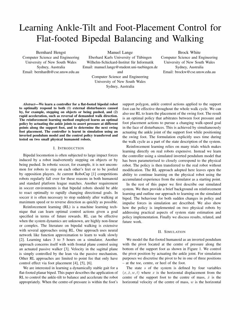
We model the flat-footed humanoid as an inverted pendulumwith the pivot located at the centre of pressure along thebottom of the support foot as shown in Figure 1. We controlthe pivot position by actuating the ankle joint. For simulationpurposes we discretise the pivot to be in one of three positions– at the toe, centre, or heel of the foot.
The state s of the system is defined by four variables(x, x, w, t) where x is the horizontal displacement from thecentre of the support foot to the centre of mass, x is thehorizontal velocity of the centre of mass, w is the horizontal
Support Foot
Swing Foot
Centre of Mass
Possible Pivot Posi-ons
Ankle Ac-va-on
Current Pivot Point
Inverted Pendulum
x w
Fig. 1. The inverted pendulum model of a flat-footed bipedal robot used forsimulation and reinforcement learning.
displacement from the centre of mass to the centre of the swingfoot, and t is the time-step from the start of each walk-cycle.
The control actions a are defined by a tuple (c, d), where cchooses the centre of pressure for the support foot relative tothe centre of the foot and d chooses a delta change in the swingfoot displacement w. We model the swing foot displacementin this way to ensure it is moved into position progressively.
The state transition function is determined by the invertedpendulum dynamics, the natural progression of time, thewalking gait that determines when the swing and support feetalternate, and the change in w based on action d. The systemdifference equations with time indexed by k and time-step ∆tare:
xk+1 = xk + xk ∆t+ xk∆t2
2(1)
xk+1 = xk + xk∆t (2)xk+1 = g sin(θk+1) cos(θk+1) (3)wk+1 = wk + d (4)tk+1 = tk + ∆t (5)
where g is the acceleration due to gravity and θk is the leanof the inverted pendulum in the clock-wise direction. Angle θis dependent on the pivot point pk determined by c and theheight of the centre of mass. The height h of the centre-of-mass of the pendulum is modelled on gait characteristics ofthe robot. We use a linear inverted pendulum – one for whichthe height of the centre of mass (CoM) is constant , henceθk = tan−1((xk − pk)/h). x
The period of a complete walk cycle is T . We assume thatthe time that the system is in a double support is small andcan be ignored for the purposes of system identification. Thesupport and swing feet alternate as the time passes throught = T/2 and t = T = 0. At these times the above transitionequations are augmented by:
xk+1 = −wk+1 (6)wk+1 = −xk+1 (7)
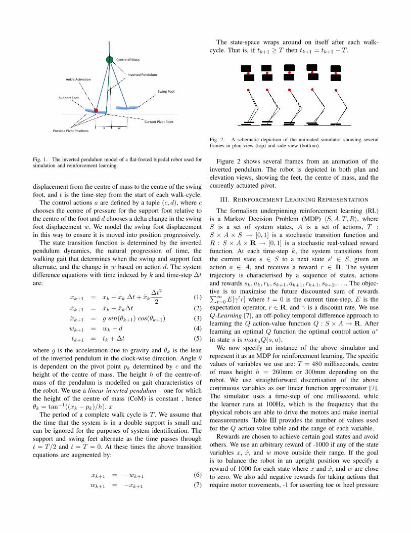
The state-space wraps around on itself after each walk-cycle. That is, if tk+1 ≥ T then tk+1 = tk+1 − T .
Fig. 2. A schematic depiction of the animated simulator showing severalframes in plan-view (top) and side-view (bottom).
Figure 2 shows several frames from an animation of theinverted pendulum. The robot is depicted in both plan andelevation views, showing the feet, the centre of mass, and thecurrently actuated pivot.
III. REINFORCEMENT LEARNING REPRESENTATION
The formalism underpinning reinforcement learning (RL)is a Markov Decision Problem (MDP) 〈S,A, T,R〉, whereS is a set of system states, A is a set of actions, T :S × A × S → [0, 1] is a stochastic transition function andR : S × A × R → [0, 1] is a stochastic real-valued rewardfunction. At each time-step k, the system transitions fromthe current state s ∈ S to a next state s′ ∈ S, given anaction a ∈ A, and receives a reward r ∈ R. The systemtrajectory is characterised by a sequence of states, actionsand rewards sk, ak, rk, sk+1, ak+1, rk+1, sk+2, . . .. The objec-tive is to maximise the future discounted sum of rewards∑∞
t=0E[γtr] where t = 0 is the current time-step, E is theexpectation operator, r ∈ R, and γ is a discount rate. We useQ-Learning [7], an off-policy temporal difference approach tolearning the Q action-value function Q : S × A → R. Afterlearning an optimal Q function the optimal control action a∗
in state s is maxaQ(s, a).We now specify an instance of the above simulator and
represent it as an MDP for reinforcement learning. The specificvalues of variables we use are: T = 480 milliseconds, centreof mass height h = 260mm or 300mm depending on therobot. We use straightforward discertisation of the abovecontinuous variables as our linear function approximator [7].The simulator uses a time-step of one millisecond, whilethe learner runs at 100Hz, which is the frequency that thephysical robots are able to drive the motors and make inertialmeasurements. Table III provides the number of values usedfor the Q action-value table and the range of each variable.
Rewards are chosen to achieve certain goal states and avoidothers. We use an arbitrary reward of -1000 if any of the statevariables x, x, and w move outside their range. If the goalis to balance the robot in an upright position we specify areward of 1000 for each state where x and x, and w are closeto zero. We also add negative rewards for taking actions thatrequire motor movements, -1 for asserting toe or heel pressure
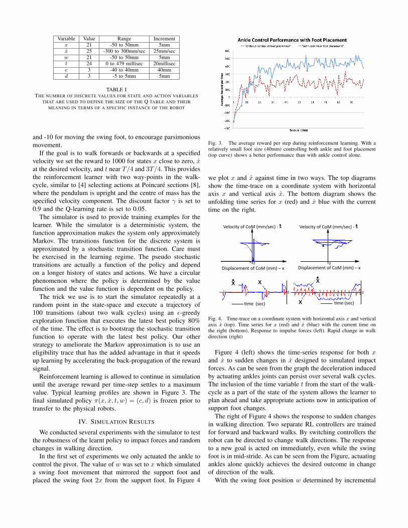
Variable Value Range Incrementx 21 -50 to 50mm 5mmx 25 -300 to 300mm/sec 25mm/secw 21 -50 to 50mm 5mmt 24 0 to 479 millisec 20millisecc 3 -40 to 40mm 40mmd 3 -5 to 5mm 5mm
TABLE ITHE NUMBER OF DISCRETE VALUES FOR STATE AND ACTION VARIABLES
THAT ARE USED TO DEFINE THE SIZE OF THE Q TABLE AND THEIRMEANING IN TERMS OF A SPECIFIC INSTANCE OF THE ROBOT
and -10 for moving the swing foot, to encourage parsimoniousmovement.
If the goal is to walk forwards or backwards at a specifiedvelocity we set the reward to 1000 for states x close to zero, xat the desired velocity, and t near T/4 and 3T/4. This providesthe reinforcement learner with two way-points in the walk-cycle, similar to [4] selecting actions at Poincare sections [8],where the pendulum is upright and the centre of mass has thespecified velocity component. The discount factor γ is set to0.9 and the Q-learning rate is set to 0.05.
The simulator is used to provide training examples for thelearner. While the simulator is a deterministic system, thefunction approximation makes the system only approximatelyMarkov. The transitions function for the discrete system isapproximated by a stochastic transition function. Care mustbe exercised in the learning regime. The pseudo stochastictransitions are actually a function of the policy and dependon a longer history of states and actions. We have a circularphenomenon where the policy is determined by the valuefunction and the value function is dependent on the policy.
The trick we use is to start the simulator repeatedly at arandom point in the state-space and execute a trajectory of100 transitions (about two walk cycles) using an ε-greedyexploration function that executes the latest best policy 80%of the time. The effect is to bootstrap the stochastic transitionfunction to operate with the latest best policy. Our otherstrategy to ameliorate the Markov approximation is to use aneligibility trace that has the added advantage in that it speedsup learning by accelerating the back-propagation of the rewardsignal.
Reinforcement learning is allowed to continue in simulationuntil the average reward per time-step settles to a maximumvalue. Typical learning profiles are shown in Figure 3. Thefinal simulated policy π(x, x, t, w) = (c, d) is frozen prior totransfer to the physical robots.
IV. SIMULATION RESULTS
We conducted several experiments with the simulator to testthe robustness of the learnt policy to impact forces and randomchanges in walking direction.
In the first set of experiments we only actuated the ankle tocontrol the pivot. The value of w was set to x which simulateda swing foot movement that mirrored the support foot andplaced the swing foot 2x from the support foot. In Figure 4
Fig. 3. The average reward per step during reinforcement learning. With arelatively small foot size (40mm) controlling both ankle and foot placement(top curve) shows a better performance than with ankle control alone.
we plot x and x against time in two ways. The top diagramsshow the time-trace on a coordinate system with horizontalaxis x and vertical axis x. The bottom diagram shows theunfolding time series for x (red) and x blue with the currenttime on the right.
Velocity of CoM (mm/sec) -‐ x Velocity of CoM (mm/sec) -‐ x
Displacement of CoM (mm) – x Displacement of CoM (mm) – x 0 0
x -me (sec) -me (sec)
0 0
x x x
Fig. 4. Time-trace on a coordinate system with horizontal axis x and verticalaxis x (top). Time series for x (red) and x (blue) with the current time onthe right (bottom). Response to impulse forces (left). Rapid change in walkdirection (right)
Figure 4 (left) shows the time-series response for both xand x to sudden changes in x designed to simulated impactforces. As can be seen from the graph the deceleration inducedby actuating ankles joints can persist over several walk cycles.The inclusion of the time variable t from the start of the walk-cycle as a part of the state of the system allows the learner toplan ahead and take appropriate actions now in anticipation ofsupport foot changes.
The right of Figure 4 shows the response to sudden changesin walking direction. Two separate RL controllers are trainedfor forward and backward walks. By switching controllers therobot can be directed to change walk directions. The responseto a new goal is acted on immediately, even while the swingfoot is in mid-stride. As can be seen from the Figure, actuatingankles alone quickly achieves the desired outcome in changeof direction of the walk.
With the swing foot position w determined by incremental
Ankle control alone Ankle and Foot-‐placement control
-me (sec)
0
x 0
x x
x
-me
Fig. 5. Time-series impulse response comparison with and without swing-foot placement control for a foot size of 40mm. The time series show bothx (red) and x (blue). Ankle control alone (left). Both ankle and swing-footplacement control (right).
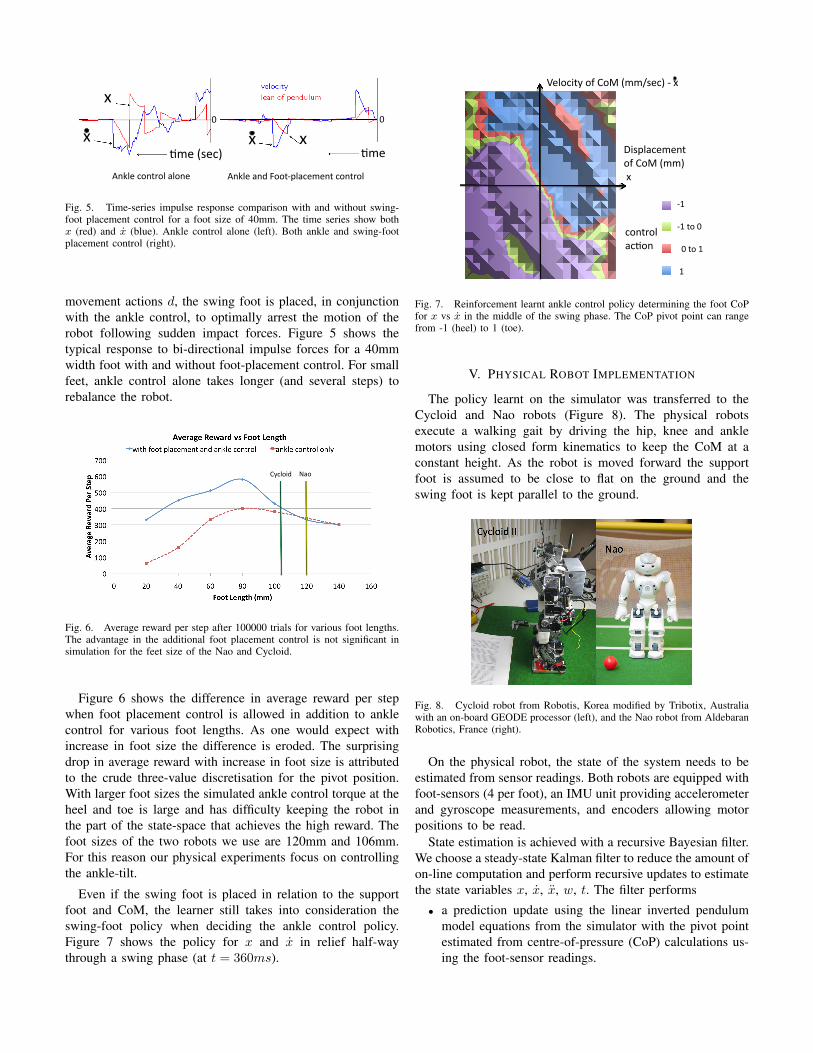
movement actions d, the swing foot is placed, in conjunctionwith the ankle control, to optimally arrest the motion of therobot following sudden impact forces. Figure 5 shows thetypical response to bi-directional impulse forces for a 40mmwidth foot with and without foot-placement control. For smallfeet, ankle control alone takes longer (and several steps) torebalance the robot.
Nao Cycloid
Fig. 6. Average reward per step after 100000 trials for various foot lengths.The advantage in the additional foot placement control is not significant insimulation for the feet size of the Nao and Cycloid.
Figure 6 shows the difference in average reward per stepwhen foot placement control is allowed in addition to anklecontrol for various foot lengths. As one would expect withincrease in foot size the difference is eroded. The surprisingdrop in average reward with increase in foot size is attributedto the crude three-value discretisation for the pivot position.With larger foot sizes the simulated ankle control torque at theheel and toe is large and has difficulty keeping the robot inthe part of the state-space that achieves the high reward. Thefoot sizes of the two robots we use are 120mm and 106mm.For this reason our physical experiments focus on controllingthe ankle-tilt.
Even if the swing foot is placed in relation to the supportfoot and CoM, the learner still takes into consideration theswing-foot policy when deciding the ankle control policy.Figure 7 shows the policy for x and x in relief half-waythrough a swing phase (at t = 360ms).
-‐1
-‐1 to 0
0 to 1
1
Velocity of CoM (mm/sec) -‐ x
Displacement of CoM (mm) x
control ac-on
Fig. 7. Reinforcement learnt ankle control policy determining the foot CoPfor x vs x in the middle of the swing phase. The CoP pivot point can rangefrom -1 (heel) to 1 (toe).
V. PHYSICAL ROBOT IMPLEMENTATION
The policy learnt on the simulator was transferred to theCycloid and Nao robots (Figure 8). The physical robotsexecute a walking gait by driving the hip, knee and anklemotors using closed form kinematics to keep the CoM at aconstant height. As the robot is moved forward the supportfoot is assumed to be close to flat on the ground and theswing foot is kept parallel to the ground.
Fig. 8. Cycloid robot from Robotis, Korea modified by Tribotix, Australiawith an on-board GEODE processor (left), and the Nao robot from AldebaranRobotics, France (right).
On the physical robot, the state of the system needs to beestimated from sensor readings. Both robots are equipped withfoot-sensors (4 per foot), an IMU unit providing accelerometerand gyroscope measurements, and encoders allowing motorpositions to be read.
State estimation is achieved with a recursive Bayesian filter.We choose a steady-state Kalman filter to reduce the amount ofon-line computation and perform recursive updates to estimatethe state variables x, x, x, w, t. The filter performs
• a prediction update using the linear inverted pendulummodel equations from the simulator with the pivot pointestimated from centre-of-pressure (CoP) calculations us-ing the foot-sensor readings.
• a correction update based on kinematic, IMU, and foot-sensor observations. The constant gain matrix used forupdating variables x, x, x, w, t is [0.5 0.5 0.5 0 0].
A. Centre of Pressure for Prediction Update
The CoP of the support foot is measured in millimetres(mm) with the origin under the ankle joint. The CoP p iscalculated by taking the weighted average of all the foot-sensorreadings of the support foot.
p(foot) =∑di ∗ fi∑fi
(8)
where foot ∈ {L(left), R(ight)}, di is the horizontal dis-tance from the ankle joint to each foot-sensor i, and fi isfoot-sensor i reading.
The CoP is used as the pivot point of the inverted pendulumfor the process update. We set the fraction of time during thewalk-cycle that each foot is in the swing phase. Over the wholewalk cycle T , the two swing phases are from t = D/4 tot = T/2−D/4 and T/2 +D/4 to T −D/4, where D is thetotal time for double support.
The support foot is determined by the sign of the coronal (orfrontal) CoP component. The coronal gait rocking motion onthe physical robot is induced by a form of bang-bang controlby switching support foot based on the zero-crossing pointof the coronal CoP measured across the support polygon ofboth feet with the origin between the feet. The period T hasbeen tuned to the natural rocking frequency of the humanoid.Coronal disturbances are corrected by adjusting the update ofthe gait time t to coincide with the zero-crossing of the coronalCoP to times t = 0 and t = T/2.
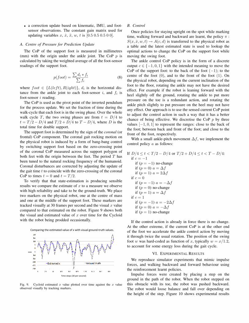
To verify that that state-estimation is producing sensibleresults we compare the estimate of x to a measure we observewith high reliability and take to be the ground-truth. We placetwo markers on the physical robot, one at the centre of massand one at the middle of the support foot. These markers aretracked visually at 30 frames per second and the visual x valuecompared to that estimated on the robot. Figure 9 shows boththe visual and estimated value of x over time for the Cycloidwith the robot being prodded occasionally.
Comparing the es-mated value of x with visual ground-‐truth values.
mm
Time-‐steps (30 per second)
Fig. 9. Cycloid estimated x value plotted over time against the x valueobserved visually by tracking markers.
B. Control
Once policies for staying upright on the spot while markingtime, walking forward and backward are learnt, the policy π :S(x, x, w, t)→ A(c, d) is transferred to the physical robot asa table and the latest estimated state is used to lookup theoptimal actions to change the CoP on the support foot whilemoving the swing foot.
The ankle control CoP policy is in the form of a discreteoutput c ∈ {−1, 0, 1} with the intended meaning to move theCoP of the support foot: to the back of the foot (−1); to thecentre of the foot (0), and to the front of the foot (1). Onthe physical robot, depending on the current inclination of thefoot to the floor, rotating the ankle may not have the desiredeffect. For example if the robot is leaning forward with theheel slightly off the ground, rotating the ankle to put morepressure on the toe is a redundant action, and rotating theankle pitch slightly to put pressure on the heel may not haveany effect. Our approach is to use the sensed current CoP pointto adjust the control action in such a way that it has a betterchance of being effective. We discretise the CoP p by threevalues [−1, 0, 1] to represent the ranges: close to the back ofthe foot; between back and front of the foot; and close to thefront of the foot, respectively.
With a small ankle-pitch movement ∆f , we implement thecontrol policy a as follows:
If D/4 ≤ t < T/2−D/4 or T/2 +D/4 ≤ t < T −D/4:if c = −1
if (p = −1) no-changeif (p = 0) a = ∆fif (p = 1) a = 2∆f
if c = 0if (p = −1) a = −∆fif (p = 0) no-changeif (p = 1) a = ∆f
if c = 1if (p = −1) a = −2∆fif (p = 0) a = −∆fif (p = 1) no-change
If the control action is already in force there is no change.At the other extreme, if the current CoP is at the other endof the foot we accelerate the ankle control action by movingit through twice the usual rotation. The position of the swingfoot w was hard-coded as function of x, typically w = x/1.2,to account for some energy loss during the gait cycle.
VI. EXPERIMENTAL RESULTS
We reproduce simulator experiments that mimic impulseforces, and walking backward and forward behaviour usingthe reinforcement learnt policies.
Impulse forces were created by placing a step on theground in the path of the robot. When the robot stepped onthis obstacle with its toe, the robot was pushed backward.The robot would loose balance and fall over depending onthe height of the step. Figure 10 shows experimental results
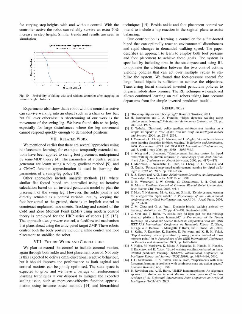
for varying step-heights with and without control. With thecontroller active the robot can reliably survive an extra 70%increase in step height. Similar trends and results are seen insimulation.
Fig. 10. Probability of falling with and without controller after stepping onvarious height obstacles.
Experiments also show that a robot with the controller activecan survive walking into an object such as a chair or low bar,but fall over otherwise. A shortcoming of our work is themovement of the swing leg. We have found this to be jerky,especially for large disturbances where the leg movementcannot respond quickly enough to demanded positions.
VII. RELATED WORK
We mentioned earlier that there are several approaches usingreinforcement learning, for example: temporally extended ac-tions have been applied to swing foot placement underpinnedby semi-MDP theory [4]. The parameters of a central patterngenerator are learnt using a policy gradient method [9], anda CMAC function approximation is used in learning theparameters of a swing-leg policy [10].
Other approaches include analytic methods [11] wheresimilar flat footed biped are controlled using an iterativecalculation based on an inverted pendulum model to plan theplacement of the swing leg. However, the ankle joint is notdirectly actuated as a control variable, but by keeping thefoot horizontal to the ground, there is an implicit control tocounteract unplanned movements. Tracking and control of theCoM and Zero Moment Point (ZMP) using modern controltheory is employed for the HRP series of robots [12] [13].The approach uses preview control, a feedforward mechanismthat plans ahead using the anticipated target ZMP. These robotscontrol both the body posture including ankle control and footplacement to stabilise the robot.
VIII. FUTURE WORK AND CONCLUSIONS
We plan to extend the control to include coronal motion,again through both ankle and foot placement control. Not onlyis this expected to deliver omni-directional reactive behaviour,but it should improve the performance as both sagittal andcoronal motions can be jointly optimised. The state space isexpected to grow and we have a barrage of reinforcementlearning techniques at our disposal to mitigate the expectedscaling issue, such as more cost-effective function approxi-mation using instance based methods [14] and hierarchical
techniques [15]. Beside ankle and foot placement control weintend to include a hip reaction in the sagittal plane to assistbalancing.
Our contribution is learning a controller for a flat-footedbiped that can optimally react to environmental disturbancesand rapid changes in demanded walking speed. The paperdescribes an approach to learn to employ both foot pressureand foot placement to achieve these goals. The system isspecified by including time in the state-space and using RLto optimise the arbitration between the two control actionsyielding policies that can act over multiple cycles to sta-bilise the system. We found that foot-pressure control forlarge footed bipeds is sufficient to achieve the objectives.Transferring learnt simulated inverted pendulum policies tophysical robots show promise. The RL technique we employedallows continued learning on real robots taking into accountdepartures from the simple inverted pendulum model.
REFERENCES
[1] “Robocup http://www.robocup.org/,” Board of Trustees, 2011.[2] H. Benbrahim and J. A. Franklin, “Biped dynamic walking using
reinforcement learning,” Robotics and Autonomous Systems, vol. 22, pp.283–302, 1997.
[3] R. Tedrake, “Stochastic policy gradient reinforcement learning on asimple 3d biped,” in Proc. of the 10th Int. Conf. on Intelligent Robotsand Systems, 2004, pp. 2849–2854.
[4] J. Morimoto, G. Cheng, C. Atkeson, and G. Zeglin, “A simple reinforce-ment learning algorithm for biped walking,” in Robotics and Automation,2004. Proceedings. ICRA ’04. 2004 IEEE International Conference on,vol. 3, april-1 may 2004, pp. 3030 – 3035 Vol.3.
[5] S. Wang and J. Braaksma, “Reinforcement learning control for bipedrobot walking on uneven surfaces,” in Proceedings of the 2006 Interna-tional Joint Conference on Neural Networks, 2006, pp. 4173–4178.
[6] J. Morimoto, J. Nakanishi, G. Endo, G. Cheng, C. G. Atkeson, andG. Zeglin, “Poincare-map-based reinforcement learning for biped walk-ing.” in ICRA’05, 2005, pp. 2381–2386.
[7] R. S. Sutton and A. G. Barto, Reinforcement Learning: An Introduction.Cambridge, Massachusetts: MIT Press, 1998.
[8] E. R. Westervelt, J. W. Grizzle, C. Chevallereau, J. H. Choi, andB. Morris, Feedback Control of Dynamic Bipedal Robot Locomotion.Boca Raton: CRC Press, 2007, vol. 1.
[9] T. Mori, Y. Nakamura, M.-A. Sato, and S. Ishii, “Reinforcement learningfor a cpg-driven biped robot,” in Proceedings of the 19th nationalconference on Artifical intelligence, ser. AAAI’04. AAAI Press, 2004,pp. 623–630.
[10] C.-M. Chew and G. A. Pratt, “Dynamic bipedal walking assisted bylearning,” Robotica, vol. 20, pp. 477–491, September 2002.
[11] C. Graf and T. Rofer, “A closed-loop 3d-lipm gait for the robocupstandard platform league humanoid,” in Proceedings of the FourthWorkshop on Humanoid Soccer Robots in conjunction with the 2010IEEE-RAS International Conference on Humanoid Robots, C. Zhou,E. Pagello, S. Behnke, E. Menegatti, T. Rofer, and P. Stone, Eds., 2010.
[12] S. Kajita, F. Kanehiro, K. Kaneko, K. Fujiwara, and K. H. K. Yokoi,“Biped walking pattern generation by using preview control of zero-moment point,” in in Proceedings of the IEEE International Conferenceon Robotics and Automation, 2003, pp. 1620–1626.
[13] S. Kajita, M. Morisawa, K. Miura, S. Nakaoka, K. Harada, K. Kaneko,F. Kanehiro, and K. Yokoi, “Biped walking stabilization based on linearinverted pendulum tracking,” IEEE/RSJ International Conference onIntelligent Robots and Systems (IROS 2010), pp. 4489–4496, 2010.
[14] J. C. Santamaria, R. S. Sutton, and A. Ram, “Experiments with rein-forcement learning in problems with continuous state and action spaces,”Adaptive Behavior, 6(2), 1998.
[15] B. Ravindran and A. G. Barto, “SMDP homomorphisms: An algebraicapproach to abstraction in semi Markov decision processes,” in Pro-ceedings of the Eighteenth International Joint Conference on ArtificialIntelligence (IJCAI 03), 2003.