Learning Bayesian Classifiers for a Visual Grammar

Selim Aksoy, Krzysztof Koperski,Carsten Tusk, Giovanni Marchisio

Insightful Corporation1700 Westlake Ave. N., Suite 500

Seattle, WA 98109, USA{saksoy,krisk,ctusk,giovanni}@insightful.com

James C. TiltonNASA Goddard Space Flight Center

Mail Code 935Greenbelt, MD 20771, USA

James.C.Tilton@nasa.gov

Abstract— A challenging problem in image content extractionand classification is building a system that automatically learnshigh-level semantic interpretations of images. We describe aBayesian framework for a visual grammar that aims to reducethe gap between low-level features and user semantics. Ourapproach includes learning prototypes of regions and their spatialrelationships for scene classification. First, naive Bayes classifiersperform automatic fusion of features and learn models forregion segmentation and classification using positive and negativeexamples for user-defined semantic land cover labels. Then, thesystem automatically learns distinguishing spatial relationshipsof these regions from training data and builds visual grammarmodels. Experiments using LANDSAT scenes show that the visualgrammar enables creation of higher level classes that cannot bemodeled by individual pixels or regions. Furthermore, learningof the classifiers requires only a few training examples.

I. INTRODUCTION

Automatic content extraction, classification and content-based retrieval are highly desired goals in intelligent databasesfor remotely sensed imagery. Most of the previous approachesuse spectral and textural features to build classification andretrieval models. However, there is a large semantic gapbetween low-level features and high-level user expectationsand scenarios.

An important element of image understanding is the spatialinformation. Traditional region or scene level image analy-sis algorithms assume that the regions or scenes consist ofuniform pixel feature distributions. However, complex queryscenarios usually contain many pixels and regions that havedifferent feature characteristics. Furthermore, two scenes withsimilar regions can have very different interpretations if theregions have different spatial arrangements. Even when pixelsand regions can be identified correctly, manual interpretationis often necessary for many applications of remote sensingimage analysis like land cover classification and ecologicalanalysis in public health studies [1]. These applications willbenefit greatly if a system can automatically learn high-levelsemantic interpretations.

The VISIMINE system [2] we have developed supportsinteractive classification and retrieval of remote sensing imagesby modeling them on pixel, region and scene levels. Pixellevel characterization provides classification details for eachpixel with regard to its spectral, textural and other ancillaryattributes. Following a segmentation process, region level

This work is supported by the NASA contract NAS5-01123.

features describe properties shared by groups of pixels. Scenelevel features model the spatial relationships of the regionscomposing a scene using a visual grammar. This hierarchicalscene modeling with a visual grammar aims to bridge the gapbetween features and semantic interpretation.

This paper describes our work on learning a visual gram-mar for scene classification. Our approach includes learningprototypes of primitive regions and their spatial relationshipsfor higher-level content extraction. Bayesian classifiers thatrequire only a few training examples are used in the learningprocess. Early work on modeling spatial relationships of re-gions include using centroid locations and minimum boundingrectangles to compute absolute and relative locations [3] orusing four quadrants of the Cartesian coordinate system tocompute directional relationships [4]. Centroids and minimumbounding rectangles are useful when regions have circularor rectangular shapes but regions in natural scenes often donot follow these assumptions. More complex representationsof spatial relationships include spatial association networks[5], knowledge-based spatial models [6], [7], and attributedrelational graphs [8]. However, these approaches require eithermanual delineation of regions by experts or partitioning ofimages into grids. Therefore, they are not generally applicabledue to the infeasibility of manual annotation in large databasesor because of the limited expressiveness of fixed sized grids.

Our work differs from other approaches in that recognitionof regions and decomposition of scenes are done automaticallyafter the system learns region and scene models with only asmall amount of supervision in terms of positive and negativeexamples for classes of interest. The rest of the paper isorganized as follows. An overview of the visual grammar isgiven in Section II. The concept of prototype regions is definedin Section III. Spatial relationships of these prototype regionsare described in Section IV. Image classification using thevisual grammar models is discussed in Section V. Conclusionsare given in Section VI.

II. VISUAL GRAMMAR

We are developing a visual grammar [9], [10] for inter-active classification and retrieval in remote sensing imagedatabases. This visual grammar uses hierarchical modelingof scenes in three levels: pixel level, region level and scenelevel. Pixel level representations include labels for individual

2120-7803-8350--8/04/$20.00 (C) 2004 IEEE.

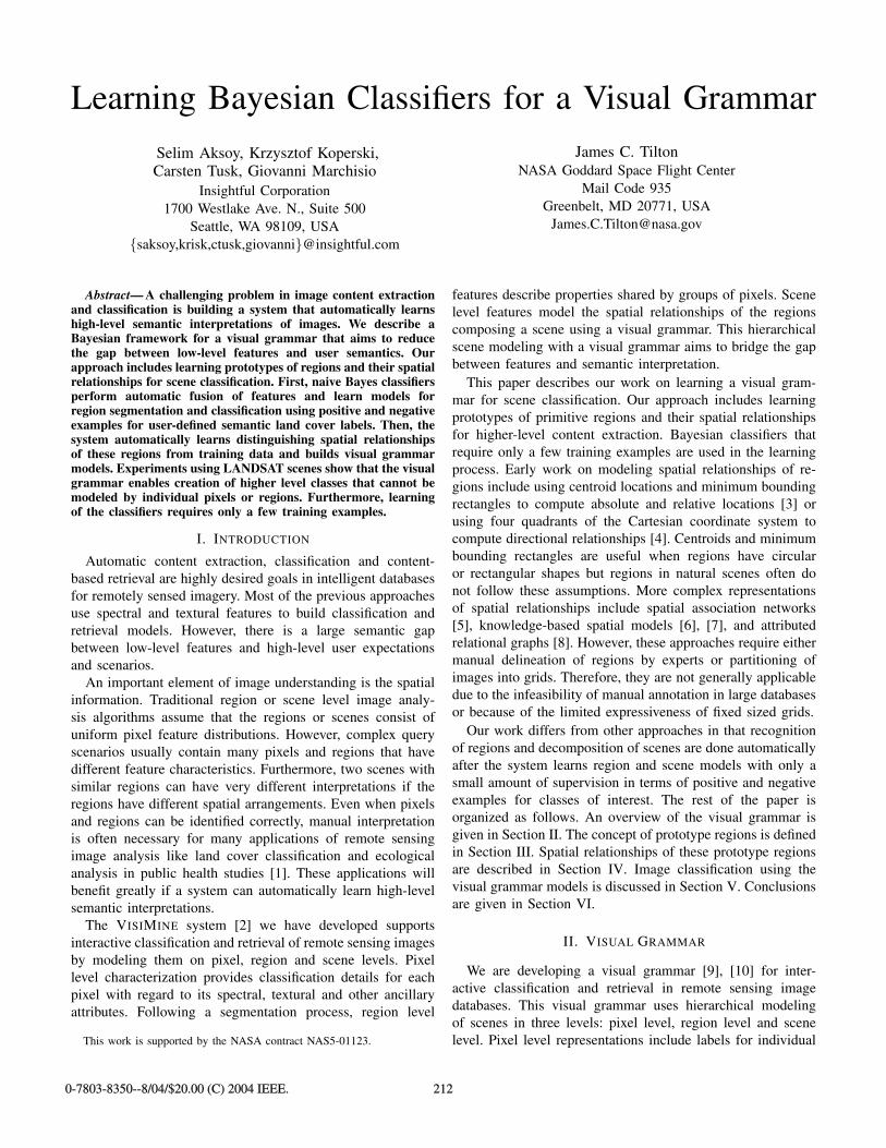
(a) NASA dataset (b) PRISM dataset

Fig. 1. LANDSAT scenes used in the experiments.

pixels computed in terms of spectral features, Gabor and co-occurrence texture features, and elevation information fromDigital Elevation Model (DEM) data. Region level represen-tations include land cover labels for groups of pixels obtainedthrough segmentation. These labels are learned from statisticalsummaries of pixel contents of regions using mean, standarddeviation and histograms, and from shape information likearea, boundary roughness, orientation and moments. Scenelevel representations include interactions of different regionscomputed in terms of spatial relationships.

Visual grammar consists of two learning steps. First, pixellevel models are learned using naive Bayes classifiers thatprovide a probabilistic link between low-level image featuresand high-level user-defined semantic labels. Then, these pixelsare merged using region growing to find region level labels.Second, a Bayesian framework is used to learn scene classesbased on automatic selection of distinguishing spatial relation-ships between regions. Details of these learning algorithms aregiven in the following sections. Examples in the rest of thepaper use LANDSAT scenes of Washington, D.C., obtainedfrom the NASA Goddard Space Flight Center, and WashingtonState and Southern British Columbia obtained from the PRISMproject at the University of Washington. We use spectral val-ues, Gabor texture features [11] and hierarchical segmentationfeatures [12] for the first dataset, and spectral values, Gaborfeatures and DEM data for the second dataset, shown in Fig. 1.

III. PROTOTYPE REGIONS

The first step to construct a visual grammar is to findmeaningful and representative regions in an image. Automaticextraction of regions is required to handle large amounts ofdata. To mimic the identification of regions by experts, wedefine the concept of prototype regions. A prototype region isa region that has a relatively uniform low-level pixel featuredistribution and describes a simple scene or part of a scene.

Ideally, a prototype is frequently found in a specific class ofscenes and differentiates this class of scenes from others.

In previous work [9], [10], we used automatic image seg-mentation and unsupervised model-based clustering to auto-mate the process of finding prototypes. In this paper, weextend this prototype framework to learn prototype modelsusing Bayesian classifiers with automatic fusion of features.Bayesian classifiers allow subjective prototype definitions tobe described in terms of objective attributes. These attributescan be based on spectral values, texture, shape, etc. Bayesianframework is a probabilistic tool to combine information frommultiple sources in terms of conditional and prior probabilities.We can create a probabilistic link between low-level imagefeatures and high-level user-defined semantic land cover labels(e.g. city, forest, field).

Assume there are k prototype labels defined by the user. Letx1, . . . , xm be the attributes computed for a pixel. The goal isto find the most probable prototype label for that pixel givena particular set of values of these attributes. The degree ofassociation between the pixel and prototype j can be computedusing the posterior probability

p(j|x1, . . . , xm)

=p(x1, . . . , xm|j)p(j)

p(x1, . . . , xm)

=p(x1, . . . , xm|j)p(j)

p(x1, . . . , xm|j)p(j) + p(x1, . . . , xm|¬j)p(¬j)

=p(j)

∏mi=1 p(xi|j)

p(j)∏m

i=1 p(xi|j) + p(¬j)∏m

i=1 p(xi|¬j)

(1)

under the conditional independence assumption. The parame-ters for each attribute model p(xi|j) can be estimated sepa-rately and this simplifies learning. Therefore, user interactionis only required for the labeling of pixels as positive (j) ornegative (¬j) examples for a particular prototype label undertraining. Then, the predicted prototype becomes the one withthe largest posterior probability and the pixel is assigned theprototype label

j∗ = arg maxj=1,...,k

p(j|x1, . . . , xm). (2)

We use discrete variables in the Bayesian model wherecontinuous features are converted to discrete attribute valuesusing an unsupervised clustering stage based on the k-meansalgorithm. In the following, we describe learning of the modelsfor p(xi|j) using the positive training examples for the j’thprototype label. Learning of p(xi|¬j) is done the same wayusing the negative examples.

For a particular prototype, let each discrete variable xi haveri possible values (states) with probabilities

p(xi = z|θi) = θiz > 0 (3)

where z ∈ {1, . . . , ri} and θi = {θiz}riz=1 is the set of

parameters for the i’th attribute model. This corresponds toa multinomial distribution. To be able to do estimation witha very small training set D, we use the conjugate prior, theDirichlet distribution p(θi) = Dir(θi|αi1, . . . , αiri

) where αiz

213

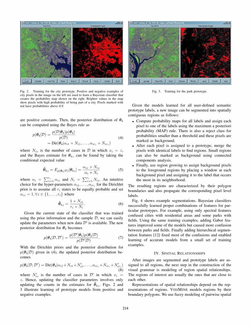
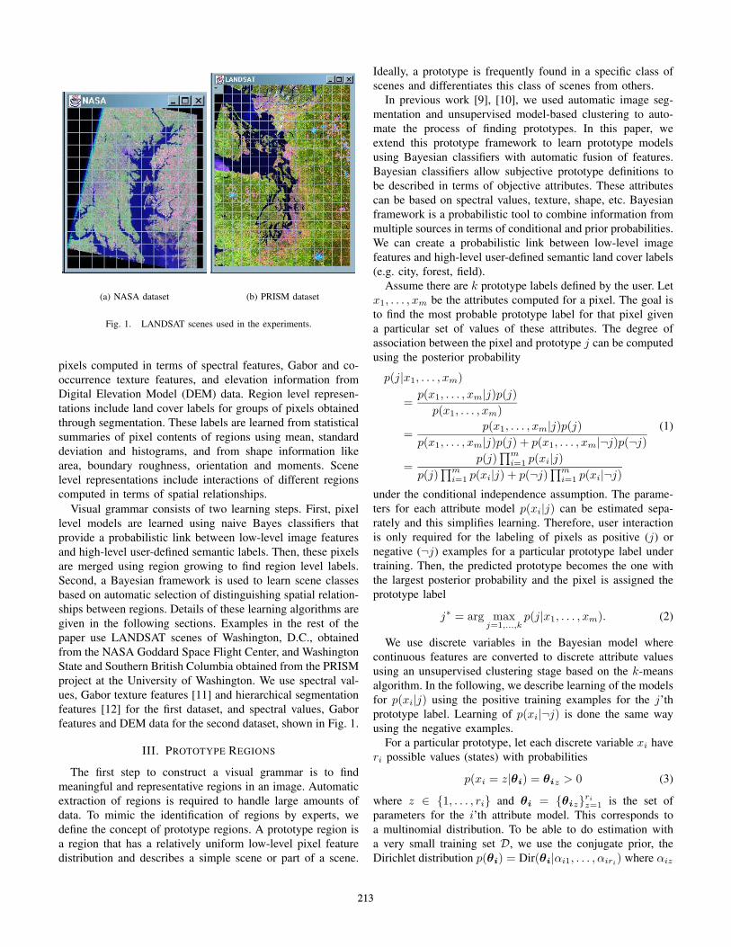
Fig. 2. Training for the city prototype. Positive and negative examples ofcity pixels in the image on the left are used to learn a Bayesian classifier thatcreates the probability map shown on the right. Brighter values in the mapshow pixels with high probability of being part of a city. Pixels marked withred have probabilities above 0.9.

are positive constants. Then, the posterior distribution of θi

can be computed using the Bayes rule as

p(θi|D) =p(D|θi)p(θi)

p(D)= Dir(θi|αi1 + Ni1, . . . , αiri

+ Niri)

(4)

where Niz is the number of cases in D in which xi = z,and the Bayes estimate for θiz can be found by taking theconditional expected value

θ̂iz = Ep(θi|D)[θiz] =αiz + Niz

αi + Ni(5)

where αi =∑ri

z=1 αiz and Ni =∑ri

z=1 Niz . An intuitivechoice for the hyper-parameters αi1, . . . , αiri

for the Dirichletprior is to assume all ri states to be equally probable and setαiz = 1,∀z ∈ {1, . . . , ri} where

θ̂iz =1 + Niz

ri + Ni. (6)

Given the current state of the classifier that was trainedusing the prior information and the sample D, we can easilyupdate the parameters when new data D′ is available. The newposterior distribution for θi becomes

p(θi|D,D′) =p(D′|θi)p(θi|D)

p(D′|D). (7)

With the Dirichlet priors and the posterior distribution forp(θi|D) given in (4), the updated posterior distribution be-comes

p(θi|D,D′) = Dir(θi|αi1+Ni1+N ′i1, . . . , αiri

+Niri+N ′

iri)

(8)where N ′

iz is the number of cases in D′ in which xi =z. Hence, updating the classifier parameters involves onlyupdating the counts in the estimates for θ̂iz . Figs. 2 and3 illustrate learning of prototype models from positive andnegative examples.

Fig. 3. Training for the park prototype.

Given the models learned for all user-defined semanticprototype labels, a new image can be segmented into spatiallycontiguous regions as follows:

• Compute probability maps for all labels and assign eachpixel to one of the labels using the maximum a posterioriprobability (MAP) rule. There is also a reject class forprobabilities smaller than a threshold and these pixels aremarked as background.

• After each pixel is assigned to a prototype, merge thepixels with identical labels to find regions. Small regionscan also be marked as background using connectedcomponents analysis.

• Finally, use region growing to assign background pixelsto the foreground regions by placing a window at eachbackground pixel and assigning it to the label that occursthe most in its neighborhood.

The resulting regions are characterized by their polygonboundaries and also propagate the corresponding pixel levellabels.

Fig. 4 shows example segmentations. Bayesian classifierssuccessfully learned proper combinations of features for par-ticular prototypes. For example, using only spectral featuresconfused cities with residential areas and some parks withfields. Using the same training examples, adding Gabor fea-tures improved some of the models but caused more confusionbetween parks and fields. Finally adding hierarchical segmen-tation features [12] fixed most of the confusions and enabledlearning of accurate models from a small set of trainingexamples.

IV. SPATIAL RELATIONSHIPS

After images are segmented and prototype labels are as-signed to all regions, the next step in the construction of thevisual grammar is modeling of region spatial relationships.The regions of interest are usually the ones that are close toeach other.

Representations of spatial relationships depend on the rep-resentations of regions. VISIMINE models regions by theirboundary polygons. We use fuzzy modeling of pairwise spatial

214

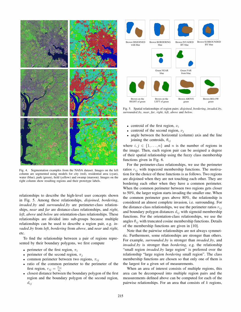
Fig. 4. Segmentation examples from the NASA dataset. Images on the leftcolumn are segmented using models for city (red), residential area (cyan),water (blue), park (green), field (yellow) and swamp (maroon). Images on theright column show resulting regions and their prototype labels.

relationships to describe the high-level user concepts shownin Fig. 5. Among these relationships, disjoined, bordering,invaded by and surrounded by are perimeter-class relation-ships, near and far are distance-class relationships, and right,left, above and below are orientation-class relationships. Theserelationships are divided into sub-groups because multiplerelationships can be used to describe a region pair, e.g. in-vaded by from left, bordering from above, and near and right,etc.

To find the relationship between a pair of regions repre-sented by their boundary polygons, we first compute

• perimeter of the first region, πi

• perimeter of the second region, πj

• common perimeter between two regions, πij

• ratio of the common perimeter to the perimeter of thefirst region, rij = πij

πi

• closest distance between the boundary polygon of the firstregion and the boundary polygon of the second region,dij

Fig. 5. Spatial relationships of region pairs: disjoined, bordering, invaded by,surrounded by, near, far, right, left, above and below.

• centroid of the first region, νi

• centroid of the second region, νj

• angle between the horizontal (column) axis and the linejoining the centroids, θij

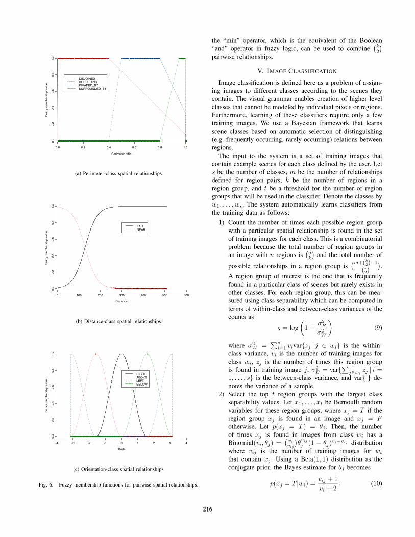
where i, j ∈ {1, . . . , n} and n is the number of regions inthe image. Then, each region pair can be assigned a degreeof their spatial relationship using the fuzzy class membershipfunctions given in Fig. 6.

For the perimeter-class relationships, we use the perimeterratios rij with trapezoid membership functions. The motiva-tion for the choice of these functions is as follows. Two regionsare disjoined when they are not touching each other. They arebordering each other when they have a common perimeter.When the common perimeter between two regions gets closerto 50%, the larger region starts invading the smaller one. Whenthe common perimeter goes above 80%, the relationship isconsidered an almost complete invasion, i.e. surrounding. Forthe distance-class relationships, we use the perimeter ratios rij

and boundary polygon distances dij with sigmoid membershipfunctions. For the orientation-class relationships, we use theangles θij with truncated cosine membership functions. Detailsof the membership functions are given in [10].

Note that the pairwise relationships are not always symmet-ric. Furthermore, some relationships are stronger than others.For example, surrounded by is stronger than invaded by, andinvaded by is stronger than bordering, e.g. the relationship“small region invaded by large region” is preferred over therelationship “large region bordering small region”. The classmembership functions are chosen so that only one of them isthe largest for a given set of measurements.

When an area of interest consists of multiple regions, thisarea can be decomposed into multiple region pairs and themeasurements defined above can be computed for each of thepairwise relationships. For an area that consists of k regions,

215

Perimeter ratio

Fuz

zy m

embe

rshi

p va

lue

0.0 0.2 0.4 0.6 0.8 1.0

0.0

0.2

0.4

0.6

0.8

1.0

DISJOINEDBORDERINGINVADED_BYSURROUNDED_BY

(a) Perimeter-class spatial relationships

Distance

Fuz

zy m

embe

rshi

p va

lue

0 100 200 300 400 500 600

0.0

0.2

0.4

0.6

0.8

1.0

FARNEAR

(b) Distance-class spatial relationships

Theta

Fuz

zy m

embe

rshi

p va

lue

-4 -3 -2 -1 0 1 2 3 4

0.0

0.2

0.4

0.6

0.8

1.0

RIGHTABOVELEFTBELOW

(c) Orientation-class spatial relationships

Fig. 6. Fuzzy membership functions for pairwise spatial relationships.

the “min” operator, which is the equivalent of the Boolean“and” operator in fuzzy logic, can be used to combine

(k2

)pairwise relationships.

V. IMAGE CLASSIFICATION

Image classification is defined here as a problem of assign-ing images to different classes according to the scenes theycontain. The visual grammar enables creation of higher levelclasses that cannot be modeled by individual pixels or regions.Furthermore, learning of these classifiers require only a fewtraining images. We use a Bayesian framework that learnsscene classes based on automatic selection of distinguishing(e.g. frequently occurring, rarely occurring) relations betweenregions.

The input to the system is a set of training images thatcontain example scenes for each class defined by the user. Lets be the number of classes, m be the number of relationshipsdefined for region pairs, k be the number of regions in aregion group, and t be a threshold for the number of regiongroups that will be used in the classifier. Denote the classes byw1, . . . , ws. The system automatically learns classifiers fromthe training data as follows:

1) Count the number of times each possible region groupwith a particular spatial relationship is found in the setof training images for each class. This is a combinatorialproblem because the total number of region groups inan image with n regions is

(nk

)and the total number of

possible relationships in a region group is(m+(k

2)−1

(k2)

).

A region group of interest is the one that is frequentlyfound in a particular class of scenes but rarely exists inother classes. For each region group, this can be mea-sured using class separability which can be computed interms of within-class and between-class variances of thecounts as

ς = log(

1 +σ2

B

σ2W

)(9)

where σ2W =

∑si=1 vivar{zj | j ∈ wi} is the within-

class variance, vi is the number of training images forclass wi, zj is the number of times this region groupis found in training image j, σ2

B = var{∑j∈wizj | i =

1, . . . , s} is the between-class variance, and var{·} de-notes the variance of a sample.

2) Select the top t region groups with the largest classseparability values. Let x1, . . . , xt be Bernoulli randomvariables for these region groups, where xj = T if theregion group xj is found in an image and xj = Fotherwise. Let p(xj = T ) = θj . Then, the numberof times xj is found in images from class wi has aBinomial(vi, θj) =

(vi

vij

)θ

vij

j (1 − θj)vi−vij distributionwhere vij is the number of training images for wi

that contain xj . Using a Beta(1, 1) distribution as theconjugate prior, the Bayes estimate for θj becomes

p(xj = T |wi) =vij + 1vi + 2

. (10)

216

Using a similar procedure with Multinomial and Dirich-let distributions, the Bayes estimate for an image be-longing to class wi (i.e. containing the scene defined byclass wi) is computed as

p(wi) =vi + 1∑si=1 vi + s

. (11)

3) For an unknown image, search for each of the t regiongroups (determine whether xj = T or xj = F, ∀j) andassign that image to the best matching class using theMAP rule with the conditional independence assumptionas

w∗ = arg maxwi

p(wi|x1, . . . , xt)

= arg maxwi

p(wi)t∏

j=1

p(xj |wi).(12)

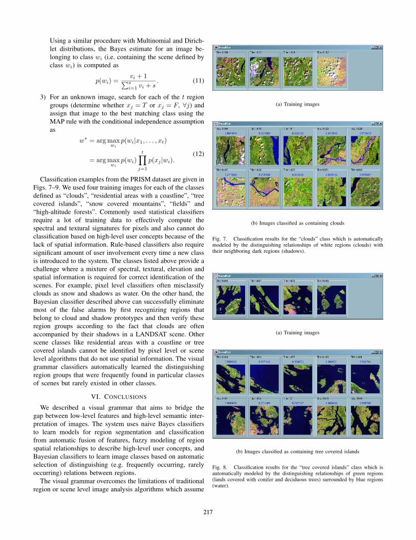
Classification examples from the PRISM dataset are given inFigs. 7–9. We used four training images for each of the classesdefined as “clouds”, “residential areas with a coastline”, “treecovered islands”, “snow covered mountains”, “fields” and“high-altitude forests”. Commonly used statistical classifiersrequire a lot of training data to effectively compute thespectral and textural signatures for pixels and also cannot doclassification based on high-level user concepts because of thelack of spatial information. Rule-based classifiers also requiresignificant amount of user involvement every time a new classis introduced to the system. The classes listed above provide achallenge where a mixture of spectral, textural, elevation andspatial information is required for correct identification of thescenes. For example, pixel level classifiers often misclassifyclouds as snow and shadows as water. On the other hand, theBayesian classifier described above can successfully eliminatemost of the false alarms by first recognizing regions thatbelong to cloud and shadow prototypes and then verify theseregion groups according to the fact that clouds are oftenaccompanied by their shadows in a LANDSAT scene. Otherscene classes like residential areas with a coastline or treecovered islands cannot be identified by pixel level or scenelevel algorithms that do not use spatial information. The visualgrammar classifiers automatically learned the distinguishingregion groups that were frequently found in particular classesof scenes but rarely existed in other classes.

VI. CONCLUSIONS

We described a visual grammar that aims to bridge thegap between low-level features and high-level semantic inter-pretation of images. The system uses naive Bayes classifiersto learn models for region segmentation and classificationfrom automatic fusion of features, fuzzy modeling of regionspatial relationships to describe high-level user concepts, andBayesian classifiers to learn image classes based on automaticselection of distinguishing (e.g. frequently occurring, rarelyoccurring) relations between regions.

The visual grammar overcomes the limitations of traditionalregion or scene level image analysis algorithms which assume

(a) Training images

(b) Images classified as containing clouds

Fig. 7. Classification results for the “clouds” class which is automaticallymodeled by the distinguishing relationships of white regions (clouds) withtheir neighboring dark regions (shadows).

(a) Training images

(b) Images classified as containing tree covered islands

Fig. 8. Classification results for the “tree covered islands” class which isautomatically modeled by the distinguishing relationships of green regions(lands covered with conifer and deciduous trees) surrounded by blue regions(water).

217

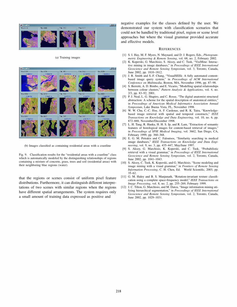
(a) Training images

(b) Images classified as containing residential areas with a coastline

Fig. 9. Classification results for the “residential areas with a coastline” classwhich is automatically modeled by the distinguishing relationships of regionscontaining a mixture of concrete, grass, trees and soil (residential areas) withtheir neighboring blue regions (water).

that the regions or scenes consist of uniform pixel featuredistributions. Furthermore, it can distinguish different interpre-tations of two scenes with similar regions when the regionshave different spatial arrangements. The system requires onlya small amount of training data expressed as positive and

negative examples for the classes defined by the user. Wedemonstrated our system with classification scenarios thatcould not be handled by traditional pixel, region or scene levelapproaches but where the visual grammar provided accurateand effective models.

REFERENCES

[1] S. I. Hay, M. F. Myers, N. Maynard, and D. J. Rogers, Eds., Photogram-metric Engineering & Remote Sensing, vol. 68, no. 2, February 2002.

[2] K. Koperski, G. Marchisio, S. Aksoy, and C. Tusk, “VisiMine: Interac-tive mining in image databases,” in Proceedings of IEEE InternationalGeoscience and Remote Sensing Symposium, vol. 3, Toronto, Canada,June 2002, pp. 1810–1812.

[3] J. R. Smith and S.-F. Chang, “VisualSEEk: A fully automated content-based image query system,” in Proceedings of ACM InternationalConference on Multimedia, Boston, MA, November 1996, pp. 87–98.

[4] S. Berretti, A. D. Bimbo, and E. Vicario, “Modelling spatial relationshipsbetween colour clusters,” Pattern Analysis & Applications, vol. 4, no.2/3, pp. 83–92, 2001.

[5] P. J. Neal, L. G. Shapiro, and C. Rosse, “The digital anatomist structuralabstraction: A scheme for the spatial description of anatomical entities,”in Proceedings of American Medical Informatics Association AnnualSymposium, Lake Buena Vista, FL, November 1998.

[6] W. W. Chu, C.-C. Hsu, A. F. Cardenas, and R. K. Taira, “Knowledge-based image retrieval with spatial and temporal constructs,” IEEETransactions on Knowledge and Data Engineering, vol. 10, no. 6, pp.872–888, November/December 1998.

[7] L. H. Tang, R. Hanka, H. H. S. Ip, and R. Lam, “Extraction of semanticfeatures of histological images for content-based retrieval of images,”in Proceedings of SPIE Medical Imaging, vol. 3662, San Diego, CA,February 1999, pp. 360–368.

[8] E. G. M. Petrakis and C. Faloutsos, “Similarity searching in medicalimage databases,” IEEE Transactions on Knowledge and Data Engi-neering, vol. 9, no. 3, pp. 435–447, May/June 1997.

[9] S. Aksoy, G. Marchisio, K. Koperski, and C. Tusk, “Probabilisticretrieval with a visual grammar,” in Proceedings of IEEE InternationalGeoscience and Remote Sensing Symposium, vol. 2, Toronto, Canada,June 2002, pp. 1041–1043.

[10] S. Aksoy, C. Tusk, K. Koperski, and G. Marchisio, “Scene modeling andimage mining with a visual grammar,” in Frontiers of Remote SensingInformation Processing, C. H. Chen, Ed. World Scientific, 2003, pp.35–62.

[11] G. M. Haley and B. S. Manjunath, “Rotation-invariant texture classifi-cation using a complete space-frequency model,” IEEE Transactions onImage Processing, vol. 8, no. 2, pp. 255–269, February 1999.

[12] J. C. Tilton, G. Marchisio, and M. Datcu, “Image information mining uti-lizing hierarchical segmentation,” in Proceedings of IEEE InternationalGeoscience and Remote Sensing Symposium, vol. 2, Toronto, Canada,June 2002, pp. 1029–1031.

218