Learning by discovering concept hierarchies

Artificial Intelligence 109 (1999) 211–242

Learning by discovering concept hierarchies

Blaž Zupana,b,∗, Marko Bohanecb,1, Janez Demšara, Ivan Bratkoa,b

a Faculty of Computer and Information Sciences, University of Ljubljana, Ljubljana, Sloveniab Department of Intelligent Systems, J. Stefan Institute, Jamova 39, SI-1000 Ljubljana, Slovenia

Received 2 April 1998

Abstract

We present a new machine learning method that, given a set of training examples, induces adefinition of the target concept in terms of a hierarchy of intermediate concepts and their definitions.This effectively decomposes the problem into smaller, less complex problems. The method is inspiredby the Boolean function decomposition approach to the design of switching circuits. To cope withhigh time complexity of finding an optimal decomposition, we propose a suboptimal heuristicalgorithm. The method, implemented in programHINT (Hierarchy INduction Tool), is experimentallyevaluated using a set of artificial and real-world learning problems. In particular, the evaluationaddresses the generalization property of decomposition and its capability to discover meaningfulhierarchies. The experiments show thatHINT performs well in both respects. 1999 Elsevier ScienceB.V. All rights reserved.

Keywords:Function decomposition; Machine learning; Concept hierarchies; Concept discovery; Constructiveinduction; Generalization

1. Introduction

To solve a complex problem, one of the most general approaches is to decompose itinto smaller, less complex and more manageable subproblems. In machine learning, thisprinciple is a foundation for structured induction [45]: instead of learning a single complexclassification rule from examples, define a concept hierarchy and learn rules for each of the(sub)concepts. Shapiro [45] used structured induction for the classification of a fairly com-plex chess endgame and demonstrated that the complexity and comprehensibility (“brain-compatibility”) of the obtained solution was superior to the unstructured one. Shapiro was

∗ Corresponding author. Email: [email protected] Email: [email protected].

0004-3702/99/$ – see front matter 1999 Elsevier Science B.V. All rights reserved.PII: S0004-3702(99)00008-9

212 B. Zupan et al. / Artificial Intelligence 109 (1999) 211–242

helped by a chess master to structure his problem domain. Typically, applications of struc-tured induction involve a manual development of the hierarchy and a manual selection andclassification of examples to induce the subconcept classification rules; usually this is atiresome process that requires an active availability of a domain expert over long periodsof time. Considerable improvements in this respect may be expected from methods thatautomate or at least actively support the user in the problem decomposition task.

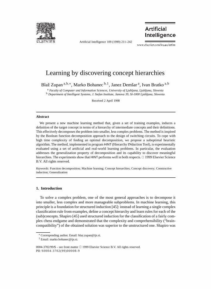
In this article we present a method for automatically developing a concept hierarchyfrom examples and investigate its applicability in machine learning. The method isimplemented in the program calledHINT (Hierarchy INduction Tool). As an illustration ofthe effectiveness of this approach, we present here some motivating experimental resultsin reconstruction of Boolean functions from examples. Consider the learning of Booleanfunctiony of five Boolean attributesx1, . . . , x5:

y = (x1 ORx2) XOR(x3 OR (x4 XOR x5)

).

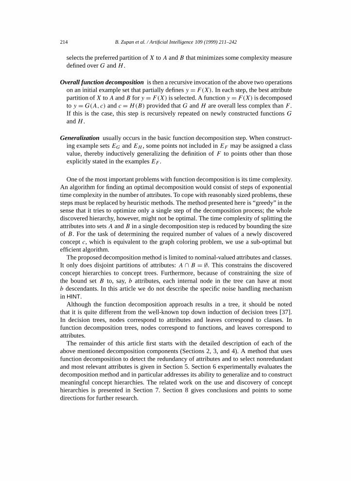
Out of the complete 5-attribute space of 32 points, 24 points (75%) were randomlyselected as examples for learning. The examples were stated as attribute-value vectors,hiding from HINT any underlying conceptual structure of the domain. In nine out of tenexperiments with different randomly selected subsets of 24 examples,HINT found thatthe most appropriate structure of subconcepts is as shown in Fig. 1.HINT also found adefinition of the intermediate functions corresponding to:

f1=OR

f2=XOR

f3=OR

f4=XOR.

This corresponds to complete reconstruction of the target concept. It should be noted thatHINT does not use any predefined repertoire of intermediate functions; the definitions ofthe four intermediate functions above were induced solely from the learning examples.

The following results show how much the detection of a useful structure in data, likethe one in Fig. 1, helps in terms of classification accuracy on new data. “New data” inour case was the remaining 25% of the points (other than those 24 examples used for

Fig. 1. Hierarchy of intermediate concepts induced byHINT for the example Boolean function.

B. Zupan et al. / Artificial Intelligence 109 (1999) 211–242 213

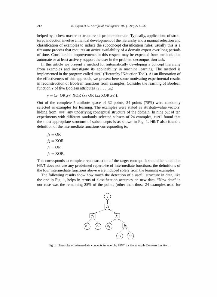
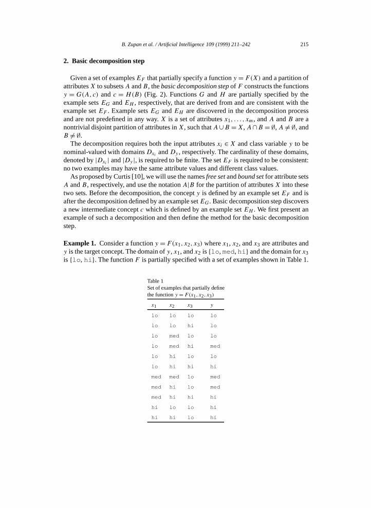
Fig. 2. Basic decomposition step.

learning). The average accuracy on new data over the 10 experiments was 97.5% withstandard deviation 7.9%. For a comparison with a “flat” learner (one that does not lookfor concept structure in data), the program C4.5 [36] was run on the same 10 datasets. Itsaccuracy was 60% with standard deviation 16.5%. This result is typical of the differencein performance betweenHINT and flat learners in similar domains where there exist usefulconcept hierarchies and illustrates dramatic effects of exploiting a possible structure in thedomain. A more thorough experimental evaluation of theHINT method is given later in thepaper.

TheHINT method is based on function decomposition, an approach originally developedfor the design of switching circuits [1,10]. The goal is to decompose a functiony = F(X)into y =G(A,H(B)), whereX is a set of input attributesx1, . . . , xm, andy is the classvariable (Fig. 2).F , G, andH are functions partially specified by examples, i.e., by setsof attribute-value vectors with assigned classes.A andB are subsets of input attributessuch thatA ∪ B = X. The functionsG andH are determined in the decompositionprocess and are not predefined in any way. Their joint complexity (determined by somecomplexity measure) should be lower than the complexity ofF . Such a decompositionalso discovers a new intermediate conceptc = H(B). Since the decomposition can beapplied recursively onH andG, the result in general is a hierarchy of concepts. For eachconcept in the hierarchy, there is a corresponding function (such asH(B)) that determinesthe dependency of that concept on its immediate descendants in the hierarchy.

A method for discovery of a concept hierarchy from an unstructured set of examplesby function decomposition can be regarded as a process that comprises the followingmechanisms:

Basic function decomposition stepwhich, given a functiony = F(X) partially repre-sented by examplesEF , and a partition of the attribute setX to setsA andB, findsthe corresponding functionsG andH , such thaty =G(A,c) andc =H(B). The newfunctions are partially defined by examplesEG andEH .

Attribute partition selection is a process which, given a functiony = F(X), examinescandidate partitions ofX toA andB and the corresponding functionsG andH . It then


selects the preferred partition ofX toA andB that minimizes some complexity measuredefined overG andH .

Overall function decompositionis then a recursive invocation of the above two operationson an initial example set that partially definesy = F(X). In each step, the best attributepartition ofX toA andB for y = F(X) is selected. A functiony = F(X) is decomposedto y =G(A,c) andc=H(B) provided thatG andH are overall less complex thanF .If this is the case, this step is recursively repeated on newly constructed functionsG

andH .

Generalization usually occurs in the basic function decomposition step. When construct-ing example setsEG andEH , some points not included inEF may be assigned a classvalue, thereby inductively generalizing the definition ofF to points other than thoseexplicitly stated in the examplesEF .

One of the most important problems with function decomposition is its time complexity.An algorithm for finding an optimal decomposition would consist of steps of exponentialtime complexity in the number of attributes. To cope with reasonably sized problems, thesesteps must be replaced by heuristic methods. The method presented here is “greedy” in thesense that it tries to optimize only a single step of the decomposition process; the wholediscovered hierarchy, however, might not be optimal. The time complexity of splitting theattributes into setsA andB in a single decomposition step is reduced by bounding the sizeof B. For the task of determining the required number of values of a newly discoveredconceptc, which is equivalent to the graph coloring problem, we use a sub-optimal butefficient algorithm.

The proposed decomposition method is limited to nominal-valued attributes and classes.It only does disjoint partitions of attributes:A ∩ B = ∅. This constrains the discoveredconcept hierarchies to concept trees. Furthermore, because of constraining the size ofthe bound setB to, say,b attributes, each internal node in the tree can have at mostb descendants. In this article we do not describe the specific noise handling mechanismin HINT.

Although the function decomposition approach results in a tree, it should be notedthat it is quite different from the well-known top down induction of decision trees [37].In decision trees, nodes correspond to attributes and leaves correspond to classes. Infunction decomposition trees, nodes correspond to functions, and leaves correspond toattributes.

The remainder of this article first starts with the detailed description of each of theabove mentioned decomposition components (Sections 2, 3, and 4). A method that usesfunction decomposition to detect the redundancy of attributes and to select nonredundantand most relevant attributes is given in Section 5. Section 6 experimentally evaluates thedecomposition method and in particular addresses its ability to generalize and to constructmeaningful concept hierarchies. The related work on the use and discovery of concepthierarchies is presented in Section 7. Section 8 gives conclusions and points to somedirections for further research.


2. Basic decomposition step

Given a set of examplesEF that partially specify a functiony = F(X) and a partition ofattributesX to subsetsA andB, thebasic decomposition stepof F constructs the functionsy = G(A,c) and c = H(B) (Fig. 2). FunctionsG andH are partially specified by theexample setsEG andEH , respectively, that are derived from and are consistent with theexample setEF . Example setsEG andEH are discovered in the decomposition processand are not predefined in any way.X is a set of attributesx1, . . . , xm, andA andB are anontrivial disjoint partition of attributes inX, such thatA∪B =X,A∩B = ∅,A 6= ∅, andB 6= ∅.

The decomposition requires both the input attributesxi ∈ X and class variabley to benominal-valued with domainsDxi andDy , respectively. The cardinality of these domains,denoted by|Dxi | and|Dy |, is required to be finite. The setEF is required to be consistent:no two examples may have the same attribute values and different class values.

As proposed by Curtis [10], we will use the namesfree setandbound setfor attribute setsA andB, respectively, and use the notationA|B for the partition of attributesX into thesetwo sets. Before the decomposition, the concepty is defined by an example setEF and isafter the decomposition defined by an example setEG. Basic decomposition step discoversa new intermediate conceptc which is defined by an example setEH . We first present anexample of such a decomposition and then define the method for the basic decompositionstep.

Example 1. Consider a functiony = F(x1, x2, x3) wherex1, x2, andx3 are attributes andy is the target concept. The domain ofy, x1, andx2 is {lo , med, hi } and the domain forx3is {lo , hi }. The functionF is partially specified with a set of examples shown in Table 1.

Table 1Set of examples that partially definethe functiony = F(x1, x2, x3)

x1 x2 x3 y

lo lo lo lo

lo lo hi lo

lo med lo lo

lo med hi med

lo hi lo lo

lo hi hi hi

med med lo med

med hi lo med

med hi hi hi

hi lo lo hi

hi hi lo hi


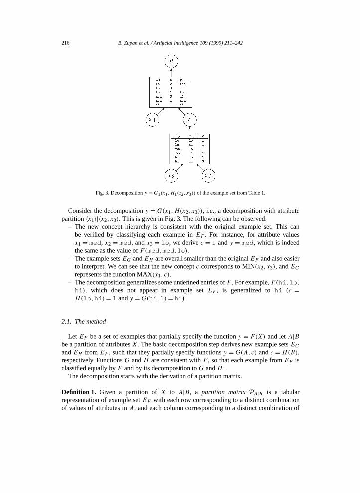
Fig. 3. Decompositiony =G1(x1,H1(x2, x3)) of the example set from Table 1.

Consider the decompositiony =G(x1,H(x2, x3)), i.e., a decomposition with attributepartition〈x1〉|〈x2, x3〉. This is given in Fig. 3. The following can be observed:

– The new concept hierarchy is consistent with the original example set. This canbe verified by classifying each example inEF . For instance, for attribute valuesx1 =med, x2 =med, andx3 = lo , we derivec = 1 andy =med, which is indeedthe same as the value ofF(med,med, lo ).

– The example setsEG andEH are overall smaller than the originalEF and also easierto interpret. We can see that the new conceptc corresponds to MIN(x2, x3), andEGrepresents the function MAX(x1, c).

– The decomposition generalizes some undefined entries ofF . For example,F(hi , lo ,

hi ), which does not appear in example setEF , is generalized tohi (c =H(lo ,hi )= 1 andy =G(hi ,1)= hi ).

2.1. The method

Let EF be a set of examples that partially specify the functiony = F(X) and letA|Bbe a partition of attributesX. The basic decomposition step derives new example setsEGandEH from EF , such that they partially specify functionsy =G(A,c) andc =H(B),respectively. FunctionsG andH are consistent withF , so that each example fromEF isclassified equally byF and by its decomposition toG andH .

The decomposition starts with the derivation of a partition matrix.

Definition 1. Given a partition ofX to A|B, a partition matrix PA|B is a tabularrepresentation of example setEF with each row corresponding to a distinct combinationof values of attributes inA, and each column corresponding to a distinct combination of


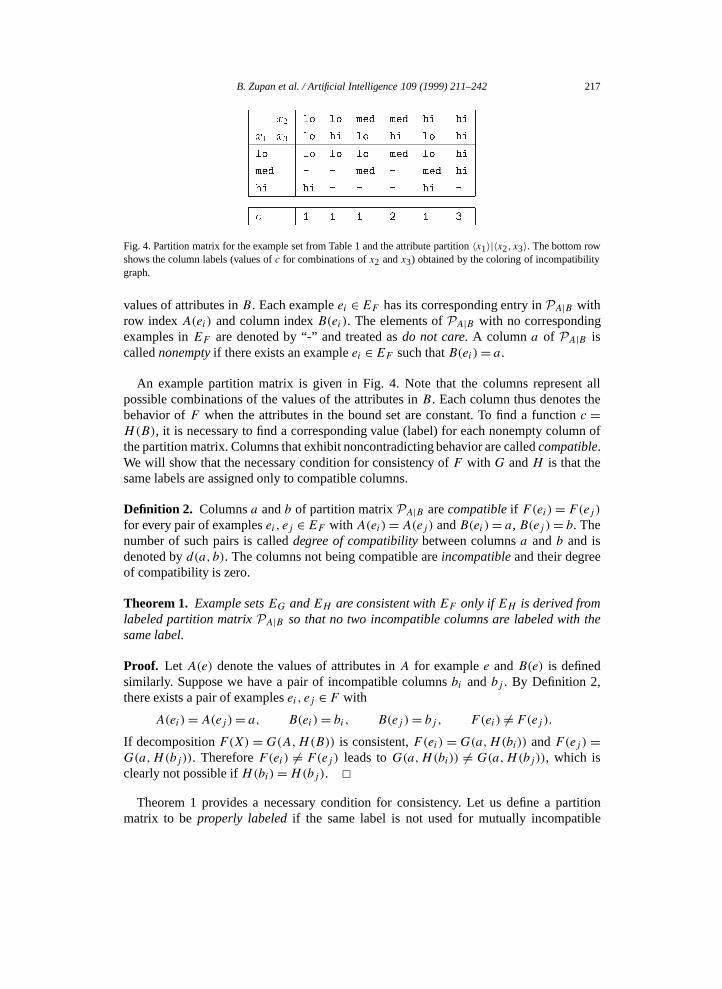
Fig. 4. Partition matrix for the example set from Table 1 and the attribute partition〈x1〉|〈x2, x3〉. The bottom rowshows the column labels (values ofc for combinations ofx2 andx3) obtained by the coloring of incompatibilitygraph.

values of attributes inB. Each exampleei ∈EF has its corresponding entry inPA|B withrow indexA(ei) and column indexB(ei). The elements ofPA|B with no correspondingexamples inEF are denoted by “-” and treated asdo not care. A columna of PA|B iscallednonemptyif there exists an exampleei ∈EF such thatB(ei)= a.

An example partition matrix is given in Fig. 4. Note that the columns represent allpossible combinations of the values of the attributes inB. Each column thus denotes thebehavior ofF when the attributes in the bound set are constant. To find a functionc =H(B), it is necessary to find a corresponding value (label) for each nonempty column ofthe partition matrix. Columns that exhibit noncontradicting behavior are calledcompatible.We will show that the necessary condition for consistency ofF with G andH is that thesame labels are assigned only to compatible columns.

Definition 2. Columnsa andb of partition matrixPA|B arecompatibleif F(ei)= F(ej )for every pair of examplesei, ej ∈EF with A(ei)=A(ej) andB(ei )= a, B(ej )= b. Thenumber of such pairs is calleddegree of compatibilitybetween columnsa andb and isdenoted byd(a, b). The columns not being compatible areincompatibleand their degreeof compatibility is zero.

Theorem 1. Example setsEG andEH are consistent withEF only ifEH is derived fromlabeled partition matrixPA|B so that no two incompatible columns are labeled with thesame label.

Proof. Let A(e) denote the values of attributes inA for examplee andB(e) is definedsimilarly. Suppose we have a pair of incompatible columnsbi andbj . By Definition 2,there exists a pair of examplesei, ej ∈ F with

A(ei)=A(ej )= a, B(ei)= bi, B(ej )= bj , F (ei) 6= F(ej ).If decompositionF(X) =G(A,H(B)) is consistent,F(ei) =G(a,H(bi)) andF(ej ) =G(a,H(bj)). ThereforeF(ei) 6= F(ej ) leads toG(a,H(bi)) 6= G(a,H(bj)), which isclearly not possible ifH(bi)=H(bj). 2

Theorem 1 provides a necessary condition for consistency. Let us define a partitionmatrix to beproperly labeledif the same label is not used for mutually incompatible


columns. Below we introduce a method that constructsEG andEH that are consistentwith EF and derived from any properly labeled partition matrix. The labeling preferredby decomposition is the one that introduces the fewest distinct labels, i.e., the one thatdefines the smallest domain for intermediate conceptsc. Finding such labeling correspondsto finding the lowest number of groups of mutually compatible columns. This number iscalledcolumn multiplicityand is denoted byν(A|B).

Definition 3. Column incompatibility graphIA|B is a graph where each nonempty columnof PA|B is represented by a vertex. Two vertices are connected if and only if thecorresponding columns are incompatible.

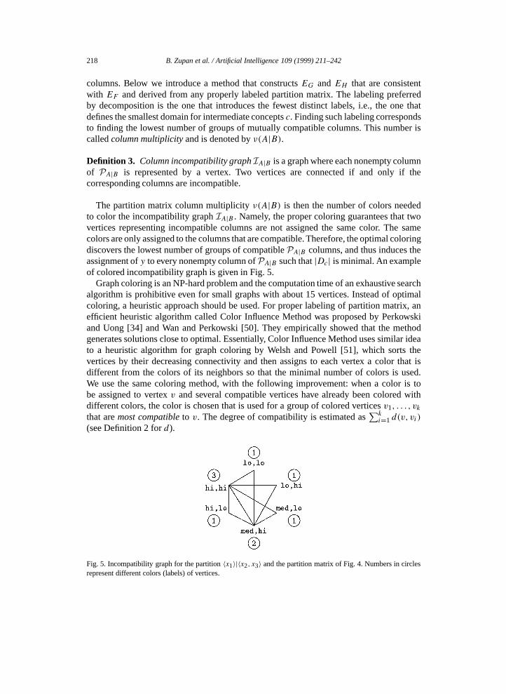
The partition matrix column multiplicityν(A|B) is then the number of colors neededto color the incompatibility graphIA|B . Namely, the proper coloring guarantees that twovertices representing incompatible columns are not assigned the same color. The samecolors are only assigned to the columns that are compatible. Therefore, the optimal coloringdiscovers the lowest number of groups of compatiblePA|B columns, and thus induces theassignment ofy to every nonempty column ofPA|B such that|Dc| is minimal. An exampleof colored incompatibility graph is given in Fig. 5.

Graph coloring is an NP-hard problem and the computation time of an exhaustive searchalgorithm is prohibitive even for small graphs with about 15 vertices. Instead of optimalcoloring, a heuristic approach should be used. For proper labeling of partition matrix, anefficient heuristic algorithm called Color Influence Method was proposed by Perkowskiand Uong [34] and Wan and Perkowski [50]. They empirically showed that the methodgenerates solutions close to optimal. Essentially, Color Influence Method uses similar ideato a heuristic algorithm for graph coloring by Welsh and Powell [51], which sorts thevertices by their decreasing connectivity and then assigns to each vertex a color that isdifferent from the colors of its neighbors so that the minimal number of colors is used.We use the same coloring method, with the following improvement: when a color is tobe assigned to vertexv and several compatible vertices have already been colored withdifferent colors, the color is chosen that is used for a group of colored verticesv1, . . . , vkthat aremost compatibleto v. The degree of compatibility is estimated as

∑ki=1 d(v, vi)

(see Definition 2 ford).

Fig. 5. Incompatibility graph for the partition〈x1〉|〈x2, x3〉 and the partition matrix of Fig. 4. Numbers in circlesrepresent different colors (labels) of vertices.


Each vertex inIA|B denotes a distinct combination of values of attributes inB, and itslabel (color) denotes a value ofc. It is therefore straightforward to derive an example setEH from the coloredIA|B . The attribute set for these examples isB. Each vertex inIA|Bis an example in setEH . Colorc of the vertex is the class of the example.

Example setEG is derived as follows. For any value ofc and combination of valuesa ofattributes inA, y =G(a, c) is determined by looking for an exampleei in row a = A(ei)and in any column labeled with the value ofc. If such an example exists, an example withattribute valuesA(ei) andc and classy = F(ei) is added toEG.

Decomposition generalizes every undefined (“-”) element ofPA|B in row a and columnb, if a corresponding exampleei with a = A(ei) and columnB(ei) with the same labelas columnb is found. For example, an undefined elementPA|B [<hi>,<lo,hi> ] of thefirst partition matrix in Fig. 4 was generalized tohi because the column<lo,hi> hadthe same label as columns<lo,lo> and<hi,lo> .

2.2. Some properties of the basic decomposition step

Here we give some properties of the basic decomposition step. We omit the proofs whichrather obviously follow from the method of constructing example setsEG andEH .

Theorem 2. The example setsEG andEH obtained by the basic decomposition step areconsistent withEF , i.e., every example inEF is correctly classified using the functionsHandG.

Theorem 3. The partition matrix column multiplicityν(A|B) obtained by optimalcoloring of IA|B is the lowest number of values forc to guarantee the consistency ofexample setsEG andEH with respect to example setEF .

Theorem 4. Let NG, NH , andNF be the numbers of examples inEG, EH , EF , res-pectively. Decomposition derivesEG andEH fromEF using the attribute partitionA|B.Then,EG and EH use fewer or the same number of attributes asEF (|B| < |X| and|A| + 16 |X|, whereX is the initial attribute set) and include fewer or the same numberof examples(NG 6NF andNH 6NF ).

2.3. Efficient derivation of the incompatibility graph

Most often, machine learning algorithms deal with sparse datasets. For these, the im-plementation using the partition matrix is memory inefficient. Instead, the incompatibilitygraphIA|B can be derived directly from the example setEF . According to Definition 3,an edge(vi , vj ) of incompatibility graphIA|B connects two verticesvi andvj if thereexist examplesek, el ∈ EF with F(ek) 6= F(el) such thatA(ek) = A(el), i = B(ek), andj = B(el). We propose an algorithm that efficiently implements the construction ofIA|Busing this definition. The algorithm first sorts the examplesEF based on the values of at-tributes inA and values ofy. Sorting uses a combination ofradix andcounting sort[9],and thus runs|A| + 1 intermediate sorts of time complexity|EF |. After sorting, the exam-


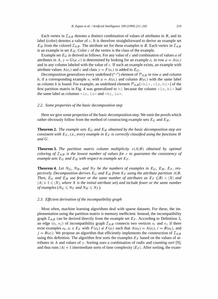
Table 2Examples from Table 1 sorted byx1 andy;double lines delimit the groups, single linesthe subgroups

x1 x2 x3 y

lo lo lo lo

lo lo hi lo

lo med lo lo

lo hi lo lo

lo med hi med

lo hi hi hi

med med lo med

med hi lo med

med hi hi hi

hi lo lo hi

hi hi lo hi

ples with the sameA(ei) constitute consecutive groups that correspond to rows in partitionmatrixPA|B . Within each group, examples with the same value ofy constitute consecutivesubgroups. Each pair of examples from the same group and different subgroups has acorresponding edge inIA|B .

Again,EH is derived directly from the coloredIA|B . The sorted examples ofEF are thenused to efficiently deriveEG. With coloring, each subgroup has obtained a label (value ofc). Each subgroup then defines a single example ofEG with the values of attributes inAand a value ofc, and a value ofy which is the same and given by any example in thesubgroup.

Example 2. For the example set from Table 1 and for the partition〈x1〉|〈x2, x3〉, theexamples sorted on the basis of the values of attributes inA and values ofy are givenin Table 2. The double lines delimit the groups and the single lines the subgroups. Nowconsider the two instances printed in bold. Their corresponding vertices inIA|B are(lo,lo) and(med,hi) . Because these instances are in the same group but in differentsubgroups, there is an edge inIA|B connecting(lo,lo) and(med,hi) .

3. Partition selection measures

The basic decomposition step assumes that a partition of the attributes to free and boundsets is given. However, for each functionF there can be many possible partitions, eachone yielding a different intermediate conceptc and a different pair of functionsG andH .


Among these partitions, we prefer those that lead to a simple conceptc and functionsGandH of low complexity.

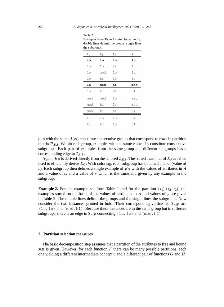
Example 3. Consider again the example set from Table 1. Its decomposition that usesthe attribute partition〈x1〉|〈x2, x3〉 is shown in Fig. 3. There are two other nontrivialattribute partitions〈x2〉|〈x1, x3〉 and 〈x3〉|〈x1, x2〉 whose decompositions are given inFig. 6. Note that, compared to these two decompositions, the first decomposition yieldsless complex and more comprehensible datasets. While we could interpret the datasetsof the first decomposition (concepts MIN and MAX), the interpretation of concepts forother two decompositions is harder. Note also that these two decompositions both discoverintermediate concepts that use more values than the one in the first decomposition. Amongthe three attribute partitions it is therefore best to decide for〈x1〉|〈x2, x3〉 and decomposey = F(x1, x2, x3) to y =G1(x1, c1) andc1=H1(x2, x3).

We introduce apartition selection measureψ(A|B) that estimates the complexity ofdecomposition ofF toG andH using the attribute partitionA|B. The best partition is theone that minimizesψ(A|B). This section introduces three partition selection measures,one based on column multiplicity of partition matrix and the remaining two based on theamount of information needed to represent the functionsG andH . The three measures areexperimentally compared in Section 6.4.

Fig. 6. The decompositionsy =G2(x2,H2(x1, x3)) andy =G3(x3,H3(x1, x2)) of the example set from Table 1.


3.1. Column multiplicity

Our simplest partition selection measure, denotedψν , is defined as the number of valuesrequired for the new featurec. That is, when decomposingF , a set of candidate partitionsis examined and one that yieldsc with the smallest set of possible values is selected fordecomposition. The number of required values forc is equal to column multiplicity ofpartition matrixPA|B , so:

ψν(A|B)= ν(A|B). (1)

Note thatν(A|B) also indirectly affects the size of instance space that definesG. Thesmaller theν(A|B), the less complex the functionG.

The idea for this measure came from practical experience with decision support systemDEX [6]. There, a hierarchical system of decision tables is constructed manually. In morethan 50 real-life applications it was observed that in order to alleviate the construction andinterpretation, the designers consistently developed functions that define concepts with asmall number of values. In most cases, they used intermediate concepts with 2 to 5 values.

Example 4. For the partitions in Fig. 4,ψν is 3, 4, and 5, respectively. As expected, thebest partition according toψν is 〈x1〉|〈x2, x3〉.

3.2. Information-based measures

The following two partition selection measures are based on the complexity of functions.Let I(F ) denote the minimal number of bits needed to encode some functionF . Then,the best partition is the one that minimizes the overall complexity of newly discoveredfunctionsH andG, i.e., the partition with minimal I(H) + I(G). The following twomeasures estimate I differently: the first one takes into account only the attribute-classspace size of the functions, while the second one additionally considers specific constraintsimposed by the decomposition over the functions.

Let us first consider some function of typey = F(X). The instance space for thisfunction is of size

|DX| =∏x∈X|Dx |. (2)

Each instance is labeled with a class value from|Dy |. Therefore, the number of all possiblefunctions in the attribute-class space is

N1(X,y)= |Dy ||DX|. (3)

Assuming the uniform distribution of functions, the number of bits to encode a functionF

is then

I1(F )= log2 N1(X,y)= |DX| log2 |Dy |. (4)

Based on I1 we can define our first information-based measureψs, which is equal to thesum of bits to encode the functionsG andH

ψs(A|B)= I1(G)+ I1(H). (5)


A similar measure for Boolean functions was proposed by Ross et al. [40] and calledDFC (Decomposed Function Cardinality). They have used it to guide the decompositionof Boolean functions and to estimate the overall complexity of derived functions. DFC ofa single function is equal to|DX|. Similarly to our definition ofψs, the DFC of a systemof functions is the sum of their DFCs.

Example 5. For the attribute partitions in Fig. 4, theψs-based partition selection measuresare:ψs(〈x1〉|〈x2, x3〉) = 23.8 bits,ψs(〈x2〉|〈x1, x3〉) = 31.0 bits, andψs(〈x3〉|〈x1, x2〉) =36.7 bits. The preferred partition is again〈x1〉|〈x2, x3〉.

When y = F(X) is decomposed toy = G(A,c) and c = H(B), the functionH isactually constrained so that:

– The intermediate conceptc usesexactly|Dc| values. Valid functionsH include onlythose that, among the examples that define them, use at least one for each of the valuesin Dc.

– The labels forc areabstractin the sense that they are used for internal bookkeepingonly and may be reordered or renamed. A specific functionH therefore represents|Dc|! equivalent functions.

For the first constraint, the number of functions that define the concepty with cardinality|Dy | using the set of attributesX is:

N2(X,y)= S(|DX|, |Dy |), (6)

whereS(n, r) is the number of distinct classifications ofn objects tor classes (Stirlingnumber of the second kind multiplied byr!) defined as:

S(n, r)=r∑i=0

(−1)r−i(r

i

)in. (7)

The formula is derived using the principle of inclusions and exclusions, which takes thetotal number of distributions ofn objects tor classes,rn, and subtracts the number ofdistributions with one class empty,

(r1

)(r − 1)n. The distributions which have not only one

but two classes empty were counted twice;(r2

)(r − 2)n is added to correct this. Now, the

distributions with three empty classes were subtracted three times as singles and then addedthree times again as pairs;

(r3

)(r − 3)n must be subtracted as a correction. Continuing this

way, we derive the above formula. For a detailed discussion, see [15].The number of valid functionsH is therefore N2(B, c)/|Dc|! and the number of bits to

encode a specific functionH assuming the uniform distribution of functions is:

I2(H)= log2N2(B, c)

|Dc|! . (8)

For functionG, the second of the above two constraints does not apply: outputs ofG areuniquely determined from examples that defineF and the developed functionH . We mayassume thatF uses all the values inDy , and so does the resulting functionG. Thus, thefirst constraint applies toG as well, and the number of bits to encode a specific functionG

is:

I′2(G)= log2 N2(A∪ {c}, y). (9)


The partition selection measureψc based on the above definition is therefore:

ψc(A|B)= I′2(G)+ I2(H)= log2 N2(A∪ {c}, y)+ log2

N2(B, c)

|Dc|! . (10)

This measure will, for any attribute partition, always be lower than or equal toψs.Our development ofψc was motivated by the work of Biermann et al. [2]. They found

an exact formula for counting the number of functions that can be represented by a givenconcept hierarchy.

In addition to the constraints onH andG mentioned above, Biermann et al. consideredconstraints related to the so-called reducibility of functions: ifc=G(B) is decomposition-constructed, then any functionH should be disregarded that makes any value ofc

redundant (see Definition 5 for redundancy of values). We did not incorporate theseconstraints intoψc since they would considerably complicate the computation and make itpractically infeasible. Namely, the computation of Biermann et al.’s formula is exponentialin the number of attributes and their domain sizes. Furthermore, it would require takinginto account not only the properties of the functionF and its attribute-class space, but alsothe properties of the complete concept hierarchy developed so far.

Example 6. For the attribute partitions in Fig. 4, theψc-based partition selection measuresare:ψc(〈x1〉|〈x2, x3〉) = 20.6 bits,ψc(〈x2〉|〈x1, x3〉) = 25.0 bits, andψc(〈x3〉|〈x1, x2〉) =28.5 bits. Again, the preferred partition is〈x1〉|〈x2, x3〉.

4. Overall function decomposition

The decomposition aims to discover a hierarchy of concepts defined by example sets thatare overall less complex than the initial one. Since an exhaustive search is prohibitivelycomplex, the decomposition uses a suboptimal greedy algorithm.

4.1. Decomposition algorithm

The overall decomposition algorithm (Algorithm 1) applies the basic decomposition stepover the evolving example sets in a concept hierarchy, starting with a single nonstructuredexample set. The algorithm keeps a listE of constructed example sets, which initiallycontains a complete training setEF0.

In each step (thewhile loop) the algorithm arbitrarily selects an example setEFi fromE which belongs to a single node in the evolving concept hierarchy. The algorithm triesto decomposeEFi by evaluating all candidate partitions of its attributes. To limit thecomplexity, the candidate partitions are those with the cardinality of the bound set lessthan or equal to a user defined parameterb. For all such partitions, a partition selectionmeasure is determined and the best partitionAbest|Bbest is selected accordingly. Next, thedecomposition determines if the best partition would result in two new example sets oflower complexity than the example setEFi being decomposed. If this is the case,EFi iscalleddecomposableand is replaced by two new example sets. This decomposition stepis then repeated until a concept structure is found that includes only nondecomposableexample sets.


Input: Set of examplesEF0 describing a single output conceptOutput: Its hierarchical decomposition

initialize E←{EF0}initialize j← 1while E 6= ∅

arbitrarily selectEFi ∈ E that partially specifiesci = Fi(x1, . . . , xm), i < jE← E \ {EFi }Abest|Bbest= argmin

A|B ψ(A|B),whereA|B runs over all possible partitions ofX = 〈x1, . . . , xm〉such thatA∪B =X, A∩B = ∅, and|B|6 b

if EFi is decomposable usingAbest|BbestthendecomposeEFi toEG andEFj , such thatci =G(Abest, cj ) andcj = Fj (Bbest)

andEG andEFj partially specifyG andFj , respectivelyEFi ←EGif |Abest|> 1 then E← E ∪ {EFi } end ifif |Bbest|> 2 then E← E ∪ {EFj } end ifj← j + 1

end ifend while

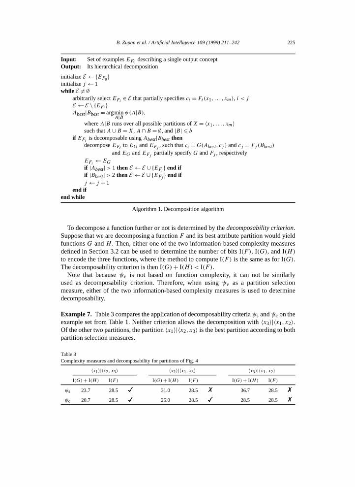
Algorithm 1. Decomposition algorithm

To decompose a function further or not is determined by thedecomposability criterion.Suppose that we are decomposing a functionF and its best attribute partition would yieldfunctionsG andH . Then, either one of the two information-based complexity measuresdefined in Section 3.2 can be used to determine the number of bits I(F ), I(G), and I(H)to encode the three functions, where the method to compute I(F ) is the same as for I(G).The decomposability criterion is then I(G)+ I(H) < I(F ).

Note that becauseψν is not based on function complexity, it can not be similarlyused as decomposability criterion. Therefore, when usingψν as a partition selectionmeasure, either of the two information-based complexity measures is used to determinedecomposability.

Example 7. Table 3 compares the application of decomposability criteriaψs andψc on theexample set from Table 1. Neither criterion allows the decomposition with〈x3〉|〈x1, x2〉.Of the other two partitions, the partition〈x1〉|〈x2, x3〉 is the best partition according to bothpartition selection measures.

Table 3Complexity measures and decomposability for partitions of Fig. 4

〈x1〉|〈x2, x3〉〈x2〉|〈x1, x3〉〈x3〉|〈x1, x2〉I(G)+ I(H) I(F ) I(G)+ I(H) I(F ) I(G)+ I(H) I(F )

ψs 23.7 28.5 31.0 28.5 36.7 28.5

ψc 20.7 28.5 25.0 28.5 28.5 28.5


4.2. Complexity of decomposition algorithm

The time complexity of a single step decomposition ofEF to EG andEH , whichconsists of sortingEF and deriving and coloring the incompatibility graph is O(Nnc)+O(Nk)+O(k2), whereN is the number of examples inEF , k is the number of vertices inIA|B , andnc is the maximum cardinality of attribute domains and domains of constructedintermediate concepts. For any bound setB, the upper bound ofk is

kmax= nbc, (11)

where b = |B|. The number of disjoint partitions considered by decomposition whendecomposingEF with n attributes is

b∑j=2

(n

j

)6

b∑j=2

nj 6 (b− 1)nb =O(nb). (12)

The highest number ofn− 2 decompositions is required when the hierarchy is a binarytree, wheren is the number of attributes in the initial example set. The time complexity ofthe decomposition algorithm is thus

O

((Nnc +Nkmax+ k2

max

) n∑m=3

mb

)=O

(nb+1(Nnc +Nkmax+ k2

max

)). (13)

Therefore, the algorithm’s complexity is polynomial inN andn, and exponential inb(kmax is exponential inb). Note that the boundb is a user-defined parameter. This analysisclearly illustrates the benefits of settingb to a sufficiently low value. In our experiments,bwas usually set to 3.

5. Attribute redundancy and decomposition-based attribute subset selection

When applying a basic decomposition step to a functiony = F(X) using some attributepartitionA|B, an interesting situation occurs when the resulting functionc = H(B) isconstant, i.e., when|Dc| = 1. For such a decomposition, the intermediate conceptc can beremoved as it does not influence the value ofy. Thus, the attributes inB areredundant,andy = F(X) can be consistently represented withy =G(A), which is a decomposition-constructed functionG(A,c) with c removed.

Such decomposition-discovered redundancy may well indicate for a true attributeredundancy. However, especially with the example sets that sparsely cover the attributespace, this redundancy may also be due to undersampling: the defined entries in partitionmatrix are sparse and do not provide the evidence for incompatibility of any two columns.In such cases, several bound sets yielding intermediate concepts with|Dc| = 1 may exist,thus misleading the partition selection measures to prefer partitions with redundant boundsets instead of those that include attributes that really define some underlying concept.

To overcome this problem, we propose an example set preprocessing by means ofattribute subset selection which removes the redundant attributes. The resulting example


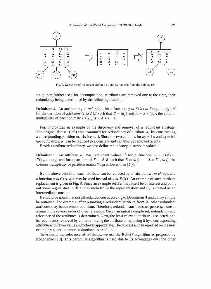
Fig. 7. Discovery of redundant attributea3 and its removal from the training set.

set is then further used for decomposition. Attributes are removed one at the time, theirredundancy being determined by the following definition.

Definition 4. An attributeaj is redundantfor a functiony = F(X) = F(a1, . . . , an), iffor the partition of attributesX to A|B such thatB = 〈aj 〉 andA=X \ 〈aj 〉, the columnmultiplicity of partition matrixPA|B is ν(A|B)= 1.

Fig. 7 provides an example of the discovery and removal of a redundant attribute.The original dataset (left) was examined for redundancy of attributea3 by constructinga corresponding partition matrix (center). Since the two columns fora3= lo anda3= hiare compatible,a3 can be reduced to a constant and can thus be removed (right).

Besides attribute redundancy, we also define redundancy in attribute values.

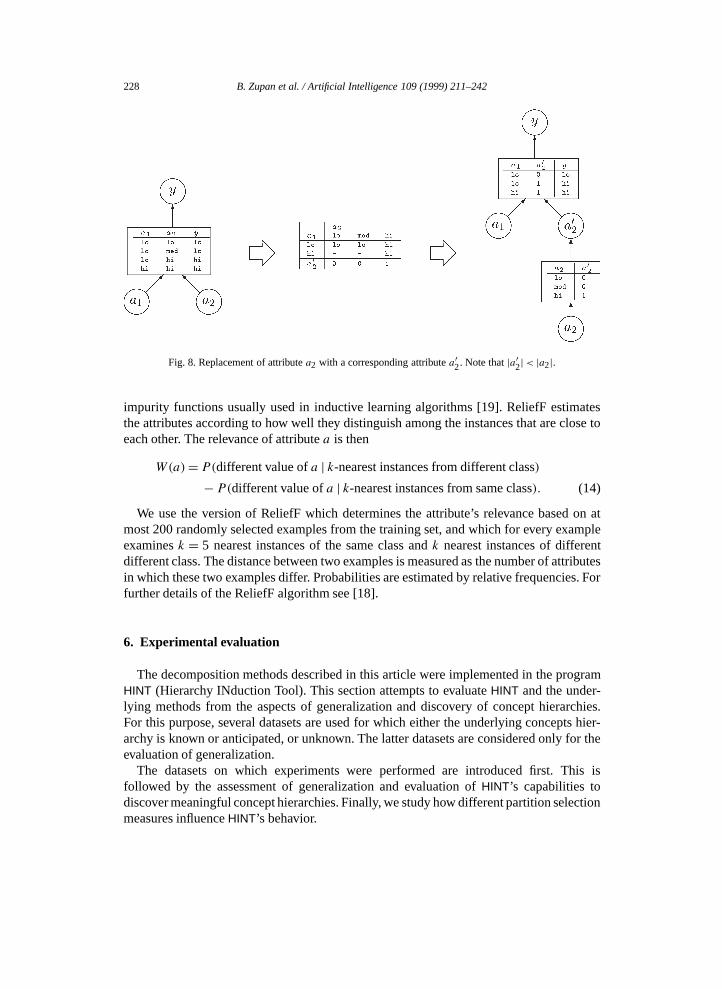
Definition 5. An attribute aj has redundant values if for a functiony = F(X) =F(a1, . . . , an) and for a partition ofX to A|B such thatB = 〈aj 〉 andA =X \ 〈aj 〉, thecolumn multiplicity of partition matrixPA|B is lower than|Dj |.

By the above definition, such attribute can be replaced by an attributea′j =H(aj), anda functiony =G(A,a′j ) may be used instead ofy = F(X). An example of such attributereplacement is given in Fig. 8. Since an example setEH may itself be of interest and pointout some regularities in data, it is included in the representation anda′j is treated as anintermediate concept.

It should be noted that not all redundancies according to Definitions 4 and 5 may simplybe removed. For example, after removing a redundant attribute fromX, other redundantattributes may become non redundant. Therefore, redundant attributes are processed one ata time in the reverse order of their relevance. Given an initial example set, redundancy andrelevance of the attributes is determined. Next, the least relevant attribute is selected, andits redundancy removed by either removing the attribute or replacing it by a correspondingattribute with fewer values, whichever appropriate. The process is then repeated on the newexample set, until no more redundancies are found.

To estimate the relevance of attributes, we use the ReliefF algorithm as proposed byKononenko [18]. This particular algorithm is used due to its advantages over the other


Fig. 8. Replacement of attributea2 with a corresponding attributea′2. Note that|a′2|< |a2|.

impurity functions usually used in inductive learning algorithms [19]. ReliefF estimatesthe attributes according to how well they distinguish among the instances that are close toeach other. The relevance of attributea is then

W(a)= P(different value ofa | k-nearest instances from different class)

− P(different value ofa | k-nearest instances from same class). (14)

We use the version of ReliefF which determines the attribute’s relevance based on atmost 200 randomly selected examples from the training set, and which for every exampleexaminesk = 5 nearest instances of the same class andk nearest instances of differentdifferent class. The distance between two examples is measured as the number of attributesin which these two examples differ. Probabilities are estimated by relative frequencies. Forfurther details of the ReliefF algorithm see [18].

6. Experimental evaluation

The decomposition methods described in this article were implemented in the programHINT (Hierarchy INduction Tool). This section attempts to evaluateHINT and the under-lying methods from the aspects of generalization and discovery of concept hierarchies.For this purpose, several datasets are used for which either the underlying concepts hier-archy is known or anticipated, or unknown. The latter datasets are considered only for theevaluation of generalization.

The datasets on which experiments were performed are introduced first. This isfollowed by the assessment of generalization and evaluation ofHINT’s capabilities todiscover meaningful concept hierarchies. Finally, we study how different partition selectionmeasures influenceHINT’s behavior.


6.1. Datasets

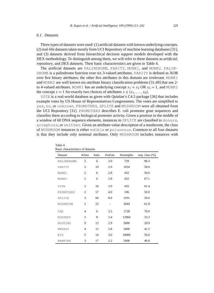
Three types of datasets were used: (1) artificial datasets with known underlying concepts,(2) real-life datasets taken mostly from UCI Repository of machine learning databases [31],and (3) datasets derived from hierarchical decision support models developed with theDEX methodology. To distinguish among them, we will refer to these datasets asartificial,repository, andDEX datasets. Their basic characteristics are given in Table 4.

The artificial datasets arePALINDROME, PARITY, MONK1, and MONK2. PALIN-DROMEis a palindrome function over six 3-valued attributes.PARITY is defined as XORover five binary attributes; the other five attributes in this domain are irrelevant.MONK1andMONK2are well known six-attribute binary classification problems [31,49] that use 2-to 4-valued attributes.MONK1has an underlying conceptx1= x2 OR x5= 1, andMONK2the conceptx = 1 for exactly two choices of attributesx ∈ {x1, . . . , x6}.

VOTEis a real-world database as given with Quinlan’s C4.5 package [36] that includesexample votes by US House of Representatives Congressmen. The votes are simplified toyes , no , or unknown . PROMOTERS, SPLICE andMUSHROOMwere all obtained fromthe UCI Repository [31].PROMOTERSdescribes E. coli promoter gene sequences andclassifies them according to biological promoter activity. Given a position in the middle ofa window of 60 DNA sequence elements, instances inSPLICE are classified todonors ,acceptors , orneither . Given an attribute-value description of a mushroom, the classof MUSHROOMinstances is eitheredible or poisonous . Common to all four datasetsis that they include only nominal attributes. OnlyMUSHROOMincludes instances with

Table 4Basic characteristics of datasets

Dataset #class #atts. #val/att. #examples maj. class (%)

PALINDROME 2 6 3.0 729 96.3

PARITY 2 10 2.0 1024 50.0

MONK1 2 6 2.8 432 50.0

MONK2 2 6 2.8 432 67.1

VOTE 2 16 3.0 435 61.4

PROMOTERS 2 57 4.0 106 50.0

SPLICE 3 60 8.0 3191 50.0

MUSHROOM 2 22 – 5644 61.8

CAR 4 6 3.5 1728 70.0

NURSERY 5 8 3.4 12960 33.3

HOUSING 9 12 2.9 5000 29.9

BREAST 4 12 2.8 5000 41.5

EIS 5 14 3.0 10000 59.0

BANKING 3 17 2.2 5000 40.8


undefined attributes, which were for the purpose of this study removed sinceHINT—asdescribed in this article—does not include explicit mechanism to handle such cases. As theconcept hierarchies for these datasets are unknown to us and neither could we anticipatethem, these datasets were only used for the study of generalization. That is, we wereinterested inHINT’s accuracy on test data.

The remaining six datasets were obtained from multi-attribute decision models origi-nally developed using DEX [6]. DEX models are hierarchical, so both the structure andintermediate concepts for these domains are known. The formalism used to describe theresulting model and its interpretation are essentially the same as those derived by decom-position. This makes models developed by DEX ideal benchmarks for the evaluation ofdecomposition. Additional convenience of DEX examples is the availability of the deci-sion support expert (Marko Bohanec) who was involved in the development of the models,for the evaluation of comprehensibility and appropriateness of the structures discovered bydecomposition.

Six different DEX models were used.CAR is a model for evaluating cars based ontheir price and technical characteristics. This simple model was developed for educationalpurposes and is described in [5].NURSERYis a real-world model developed to rankapplications for nursery schools [33].HOUSINGis a model to determine the priority ofhousing loans applications [4]. This model is a part of a management decision supportsystem for allocating housing loans that has been used since 1991 in the Housing Fund ofSlovenia.BANKING, EIS andBREASTare three previously unpublished models for theevaluation of business partners in banking, evaluation of executive information systems,and breast-cancer risk assessment, respectively.

Each DEX model was used to obtain either 5000 or 10000 attribute-value instances withcorresponding classes as derived from the model such that the class distribution was equalas in the dataset that would completely cover the attribute space. We have decided for either5000 or 10000 examples because within this rangeHINT’s behavior was found to be mostrelevant and diverse. The only exception isCARwhere 1728 instances completely coverthe attribute space.

6.2. Generalization

Here we study how the size of the training set affectsHINT’s ability to find a correctgeneralization. We construct learning curves by a variant of 10-fold cross-validation. In10-fold cross validation, the data is divided to 10 subsets, of which 9 are used for trainingand the remaining one for testing. The experiment is repeated 10 times, each time using adifferent testing subset. Stratified splits are used, i.e., the class distribution of the originaldataset and training and test sets are essentially the same. In our case, instead of learningfrom all examples from 9 subsets, onlyp percent of training instances from 9 subsetsare randomly selected for learning, wherep ranges from 10% to 100% in 10% steps. Thisadaptation of the standard method was necessary to keep test sets independent and compareclassifiers as proposed in [42]. Note that whenp = 100%, this method is equivalent to thestandard stratified 10-fold cross-validation.

HINT derived a concept hierarchy and corresponding classifier using the examples in thetraining set. The hierarchy was tested for classification accuracy on the test set. For each


p, the results are the average of 10 independent experiments. The attribute subset selectionwas used on a training set as described in Section 5. The resulting set of examples wasthen used to induce a concept hierarchy.HINT used the column multiplicity as a partitionselection measure and determined the decomposability based on our first information-based measureψν (Section 3.2). The bound set sizeb was limited to three.

The concept hierarchy obtained from training set was used to classify the instances in thetest set. The instance’s class value was obtained by bottom-up derivation of intermediateconcepts. For each intermediate concept, its example set may or may not include theappropriate example to be used for classification. In the latter case, thedefault rulewasused that assigns the value of most frequently used class in the example set that defines theintermediate concept.

We compareHINT’s learning curve to the one obtained by C4.5 inductive decision treelearner [36] run on the same data. As is the case withHINT, C4.5 was also required toinduce a decision tree consistent with the training set. Hence, C4.5 used the default optionsexcept for-m1 (minimal number of instances in leafs was set to 1) and the classificationaccuracy was evaluated on unpruned decision trees. For several datasets, we have observedthat subsetting (option-s ) obtains a more accurate classifier: the learning curves for C4.5were then developed both with and without subsetting, and the better one of the two wasused for comparison withHINT. For eachp, a binomial test [42] was used to test forsignificant differences between the methods usingα = 0.01 (99% confidence level).

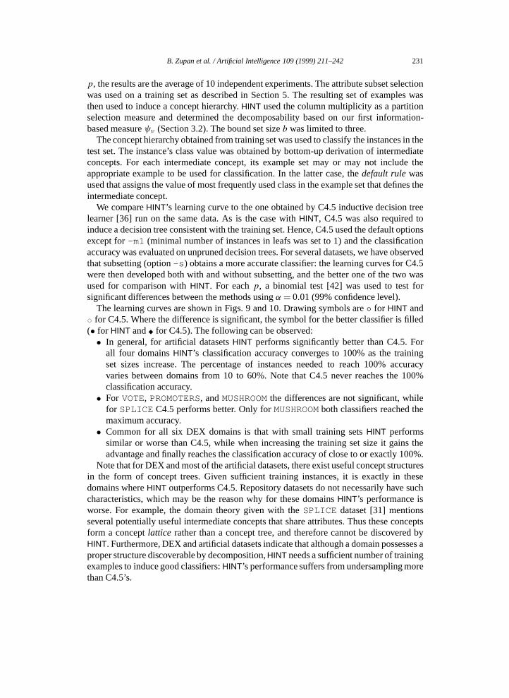
The learning curves are shown in Figs. 9 and 10. Drawing symbols are◦ for HINT andE for C4.5. Where the difference is significant, the symbol for the better classifier is filled(• for HINT andF for C4.5). The following can be observed:• In general, for artificial datasetsHINT performs significantly better than C4.5. For

all four domainsHINT’s classification accuracy converges to 100% as the trainingset sizes increase. The percentage of instances needed to reach 100% accuracyvaries between domains from 10 to 60%. Note that C4.5 never reaches the 100%classification accuracy.• For VOTE, PROMOTERS, andMUSHROOMthe differences are not significant, while

for SPLICE C4.5 performs better. Only forMUSHROOMboth classifiers reached themaximum accuracy.• Common for all six DEX domains is that with small training setsHINT performs

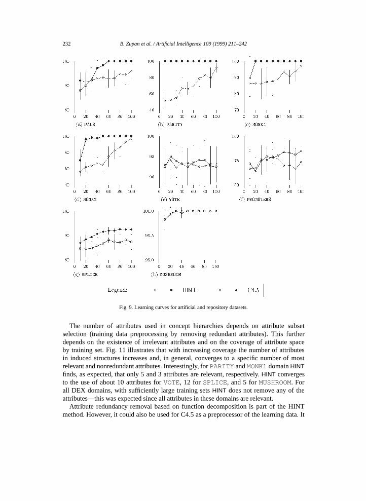
similar or worse than C4.5, while when increasing the training set size it gains theadvantage and finally reaches the classification accuracy of close to or exactly 100%.

Note that for DEX and most of the artificial datasets, there exist useful concept structuresin the form of concept trees. Given sufficient training instances, it is exactly in thesedomains whereHINT outperforms C4.5. Repository datasets do not necessarily have suchcharacteristics, which may be the reason why for these domainsHINT’s performance isworse. For example, the domain theory given with theSPLICE dataset [31] mentionsseveral potentially useful intermediate concepts that share attributes. Thus these conceptsform a conceptlattice rather than a concept tree, and therefore cannot be discovered byHINT. Furthermore, DEX and artificial datasets indicate that although a domain possesses aproper structure discoverable by decomposition,HINT needs a sufficient number of trainingexamples to induce good classifiers:HINT’s performance suffers from undersampling morethan C4.5’s.


Fig. 9. Learning curves for artificial and repository datasets.

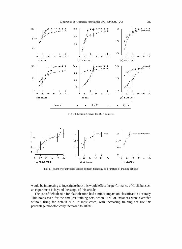
The number of attributes used in concept hierarchies depends on attribute subsetselection (training data preprocessing by removing redundant attributes). This furtherdepends on the existence of irrelevant attributes and on the coverage of attribute spaceby training set. Fig. 11 illustrates that with increasing coverage the number of attributesin induced structures increases and, in general, converges to a specific number of mostrelevant and nonredundant attributes. Interestingly, forPARITY andMONK1domainHINTfinds, as expected, that only 5 and 3 attributes are relevant, respectively.HINT convergesto the use of about 10 attributes forVOTE, 12 for SPLICE, and 5 forMUSHROOM. Forall DEX domains, with sufficiently large training setsHINT does not remove any of theattributes—this was expected since all attributes in these domains are relevant.

Attribute redundancy removal based on function decomposition is part of the HINTmethod. However, it could also be used for C4.5 as a preprocessor of the learning data. It


Fig. 10. Learning curves for DEX datasets.

Fig. 11. Number of attributes used in concept hierarchy as a function of training set size.

would be interesting to investigate how this would effect the performance of C4.5, but suchan experiment is beyond the scope of this article.

The use of default rule for classification had a minor impact on classification accuracy.This holds even for the smallest training sets, where 95% of instances were classifiedwithout firing the default rule. In most cases, with increasing training set size thispercentage monotonically increased to 100%.


6.3. Hierarchical concept structures

Induced concept structures were compared to those anticipated for artificial and DEXdomains. For each of these,HINT converged to a single concept structure when increasingthe training set size. ForPALINDROMEandPARITY, HINT induced expected structureof the type(x1 = x6 AND x2 = x5) AND (x3 = x4) and x1 XOR ((x2 XOR x3) XOR(x4 XOR x5)).

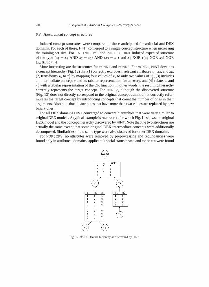
More interesting are the structures forMONK1andMONK2. ForMONK1, HINT developsa concept hierarchy (Fig. 12) that (1) correctly excludes irrelevant attributesx3, x4, andx6,(2) transformsx5 to x ′5 by mapping four values ofx5 to only two values ofx ′5, (3) includesan intermediate conceptc and its tabular representation forx1= x2, and (4) relatesc andx ′5 with a tabular representation of the OR function. In other words, the resulting hierarchycorrectly represents the target concept. ForMONK2, although the discovered structure(Fig. 13) does not directly correspond to the original concept definition, it correctly refor-mulates the target concept by introducing concepts that count the number of ones in theirarguments. Also note that all attributes that have more than two values are replaced by newbinary ones.

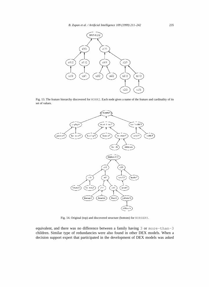
For all DEX domainsHINT converged to concept hierarchies that were very similar tooriginal DEX models. A typical example isNURSERY, for which Fig. 14 shows the originalDEX model and the concept hierarchy discovered byHINT. Note that the two structures areactually the same except that some original DEX intermediate concepts were additionallydecomposed. Similarities of the same type were also observed for other DEX domains.

For NURSERY, no attributes were removed by preprocessing and redundancies werefound only in attributes’ domains: applicant’s social statusnone andmedium were found

Fig. 12.MONK1feature hierarchy as discovered byHINT.


Fig. 13. The feature hierarchy discovered forMONK2. Each node gives a name of the feature and cardinality of itsset of values.

Fig. 14. Original (top) and discovered structure (bottom) forNURSERY.

equivalent, and there was no difference between a family having3 or more-than-3children. Similar type of redundancies were also found in other DEX models. When adecision support expert that participated in the development of DEX models was asked


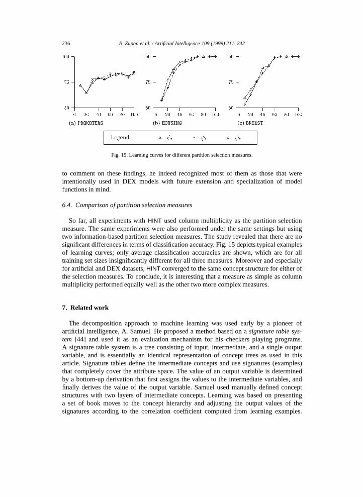
Fig. 15. Learning curves for different partition selection measures.

to comment on these findings, he indeed recognized most of them as those that wereintentionally used in DEX models with future extension and specialization of modelfunctions in mind.

6.4. Comparison of partition selection measures

So far, all experiments withHINT used column multiplicity as the partition selectionmeasure. The same experiments were also performed under the same settings but usingtwo information-based partition selection measures. The study revealed that there are nosignificant differences in terms of classification accuracy. Fig. 15 depicts typical examplesof learning curves; only average classification accuracies are shown, which are for alltraining set sizes insignificantly different for all three measures. Moreover and especiallyfor artificial and DEX datasets,HINT converged to the same concept structure for either ofthe selection measures. To conclude, it is interesting that a measure as simple as columnmultiplicity performed equally well as the other two more complex measures.

7. Related work

The decomposition approach to machine learning was used early by a pioneer ofartificial intelligence, A. Samuel. He proposed a method based on asignature table sys-tem [44] and used it as an evaluation mechanism for his checkers playing programs.A signature table system is a tree consisting of input, intermediate, and a single outputvariable, and is essentially an identical representation of concept trees as used in thisarticle. Signature tables define the intermediate concepts and use signatures (examples)that completely cover the attribute space. The value of an output variable is determinedby a bottom-up derivation that first assigns the values to the intermediate variables, andfinally derives the value of the output variable. Samuel used manually defined conceptstructures with two layers of intermediate concepts. Learning was based on presentinga set of book moves to the concept hierarchy and adjusting the output values of thesignatures according to the correlation coefficient computed from learning examples.


Compared to his previous approach that was based on the learning of the coefficients in alinear evaluation polynomial [43], Samuel showed that the use of a signature table systemsignificantly improves the performance. Samuel’s approach was later studied and improvedby Biermann et al. [2], but still required the concept structure to be given in advance.

While, within machine learning, Samuel and Biermann et al. may be the first to realizethe power of using concept hierarchies, fundamentals of the approach that can discoversuch hierarchies were defined earlier in the area of switching circuit design. Curtis [10]reports that in the late 1940s and 1950s several switching circuit theorists considered thissubject and in 1952 Ashenhurst reported on a unified theory of decomposition of switchingfunctions [1]. The method proposed by Ashenhurst decomposes the truth table of a Booleanfunction to be realized with standard binary gates. Most of other related work of that time isreported and reprinted in [10], where Curtis compares the decomposition approach to otherswitching circuit design approaches and further formalizes and extends the decompositiontheory. Besides a disjoint decomposition, where each variable can appear as input in justone of the derived tables, Curtis defines a nondisjoint decomposition where the resultingstructure is an acyclic graph rather than a tree. Furthermore, Curtis defines a decompositionalgorithm that aims at constructing a switching circuit of the lowest complexity, i.e., withthe lowest number of gates used. Curtis’ method is defined over two-valued variables andrequires a set of examples that completely cover the attribute space.

Recently, the Ashenhurst–Curtis approach was substantially improved by researchgroups of M.A. Perkowski, T. Luba, and T.D. Ross. Perkowski and Uong [34] and Wanand Perkowski [50] propose a graph coloring approach to the decomposition of incom-pletely specified switching functions. A different approach is presented by Luba and Sel-varaj [23]. Their decomposition algorithms are able to generalize. A generalization of func-tion decomposition when applied to a set of simple Boolean functions was studied by Rosset al. [40] and Goldman [14]. The authors indicate that the decomposition approach toswitching function design may be termed knowledge discovery as functions and featuresnot previously anticipated can be discovered. A similar point, but using different terminol-ogy, was made already by Curtis [10], who observed that the same truth table representinga Boolean function might have different decompositions.

Feature discovery has been at large investigated by constructive induction, a recentlyactive field within machine learning. The term was first used by Michalski [25], whodefined it as an ability of the system to derive and use new attributes in the processof learning. Following this idea and perhaps closest to function decomposition are theconstructive induction systems that use a set of constructive operators to derive newattributes. Examples of such systems are described in [24,35,38]. The main limitation ofthese approaches is that the set of constructive operators has to be defined in advance.Moreover, in constructive induction, the new features are primarily introduced for thepurpose of improving the classification accuracy of the induced classifier, while theabove described function decomposition approaches focused primarily on the reduction ofcomplexity, where the impact on classification accuracy can be regarded rather as a side-effect of decomposition-based generalization. In first-order learning of relational conceptdescriptions, constructive induction is referred to as predicate invention. An overview ofrecent achievements in this area can be found in [47].


Decomposition with nominal-valued attributes and classes may be regarded as a straight-forward extension of Ashenhurst–Curtis approach. Such an extension was described byBiermann et al. [2]. Alternatively, Luba [22] proposes a decomposition where multi-valuedintermediate concepts are binarized. Files et al. [13] propose a decomposition approach fork-valued logic where both attributes and intermediate concepts take at mostk values.

A concept structure as used in this article defines a declarative bias over the hypothesisspace. Biermann et al. [2] showed that concept structure significantly limits the numberof representable functions. This was also observed by Russell [41], who proved that tree-structured bias can reduce the size of concept language from doubly-exponential to singlyexponential in the number of attributes. Tadepalli and Russell [48] show that such biasenables PAC-learning of tabulated functions within concept structure. Their approach fordecomposition of Boolean functions requires the concept structure to be given in advance.Their learning algorithm differs from the function decomposition approaches in that ituses both examples and queries, i.e., asks the oracle for the class value of instances thatare needed in derivation but not provided in the training examples. Similar to functiondecomposition, the learning algorithm of Tadepalli and Russell induces intermediateconcepts that are lower in the hierarchy first. As with Ashenhurst–Curtis decomposition,the resulting classifiers are consistent with training examples. Queries are also used in PAC-learning described by Bshouty et al. [8]. Their algorithm identifies both concept structuresand their associated tabulated functions, but can deal only with Boolean functions withsymmetric and constant fan-in gates. Within PAC-learning, Hancock et al. [16] learnnonoverlappingperceptron networks from examples and membership queries. An excellentreview of other related work in PAC-learning that uses structural bias and queries is givenin [48].

Function decomposition is also related to construction of oblivious read-once decisiongraphs (OODG). OODGs are rooted, directed acyclic graphs that can be divided intolevels [17]. All nodes at a level test the same attribute, and all edges that originate from onelevel terminate at the next level. Like with decision trees, OODG leaf nodes represent classvalues. OODGs can be regarded as a special case of decomposition, where decompositionstructures are of the formf1(x1, f2(x2, . . . , fn(xn))) and wherexn is at the top of a decisiongraph and the number of nodes at each level equals the number of distinct output valuesused by corresponding functionfi . In fact, decision graphs were found as a good formof representation of examples to be used by decomposition [13,20,21]. Within machinelearning, the use of oblivious decision graphs was studied by Kohavi [17]. Graphs inducedby his learning algorithm are consistent with training examples, and for incomplete datasetsthe core of the algorithm is a graph coloring algorithm similar to the one defined byPerkowski and Uong [34].

Of other machine learning approaches that construct concept hierarchies we heremention Muggleton’s DUCE [29,30] which uses transformation operators to compressthe given examples by successive generalization and feature construction. Nevill-Manningand Witten [32] describe SEQUITUR, an algorithm that infers a hierarchical structurefrom a sequence of discrete symbols. Although there are some similarities with functiondecomposition (e.g., maintaining consistency and induction of new features), DUCE andSEQUITUR are essentially different in both the algorithmic and representational aspects.


Within machine learning, there are other approaches based on problem decomposition,but where the problem is decomposed by an expert and not discovered by a machine.A well-known example is structured induction, a term introduced by Donald Michie andapplied by Shapiro and Niblett [46] and Shapiro [45]. Their approach is based on amanual decomposition of the problem and an expert-assisted selection and classificationof examples to construct rules for intermediate concepts in the hierarchy. In comparisonwith standard decision tree induction techniques, structured induction exhibits about thesame classification accuracy with the increased transparency and lower complexity of thedeveloped models. Michie [26] emphasized the important role of structured induction inthe future and listed several real problems that had been solved in this way.

Mozetic [7,27,28] employed another scheme for structuring the learning problem. Thatapproach was particularly aimed at automated construction of system models from input–output observations of the system’s behavior. The structure of the learning problem,specified by a Prolog clause, corresponded to the physical structure of the modeled systemin terms of the system’s components and connections among them. In an experiment, asubstantial part of a qualitative model of the heart was induced from examples of thebehavior of the heart. It was shown that the structuring of the domain very significantlyimproved the effectiveness of learning compared to unstructured learning. Again, thestructure of the system was specified by the user and not induced automatically.

Concept hierarchy has also been used in a multi-attribute decision support expert systemshell DEX [6] which has its roots in DECMAK methodology [3,12]. There, a tree-likestructure of variables is defined by an expert, and several tools assist in the acquisitionof decision rules. These are, like Samuel’s signature tables, used to derive the valuesof intermediate and output variables. DEX also allows different representations of user-defined decision tables, including decision trees [45] and decision rules [39]. DEX hasbeen applied in more than 50 real decision making problems.

The method presented in this article essentially borrows from three different researchareas: it shares the motivation with structured induction and structured approach todecision support, while the core of the method is based on Ashenhurst–Curtis functiondecomposition. In comparison with related work, the present article is original in thefollowing respects: new method for handling multi-valued attributes and classes, improveddecomposition heuristics, treatment of redundancies, emphasis on generalization effects ofdecomposition, paying strong attention to the discovery of meaningful concept hierarchies,and experimental evaluation on machine learning problems. Our earlier experiments infunction decomposition applied to DEX domains were presented in [53,54].

8. Conclusion

We introduced a new machine learning approach based on function decomposition.A distinguishing feature of this approach is its capability to discover new intermediate con-cepts, organize them into a hierarchical structure, and induce the relationships between theattributes, newly discovered concepts, and the target concept. In their basic form, these re-lationships are specified by newly constructed example sets. In a way, the learning processcan thus be viewed as a process of generating new, equivalent example sets, which are


consistent with the original example set. The new sets are smaller, have smaller number ofattributes, and introduce intermediate concepts. Generalization also occurs in this process.

We have evaluated the decomposition-based learning method on several datasets. Inparticular, we studied the accuracy of the induced descriptions byHINT and its capabilityto discover meaningful hierarchies. For all datasets where useful hierarchies existed,HINTsignificantly outperformed C4.5 and found relevant concept hierarchies, provided thatenough examples were used for training. Experiments show that decomposition is moresensitive to undersampling and, especially in more complex datasets, C4.5 performedrelatively better with small training sets. For other datasets, with no useful conceptstructure, C4.5 andHINT performed similarly in all but one domain.

In terms of the meaningfulness of discovered structures, the most significant experimentswere those with DEX domains. For these domainsHINT’s task was to reconstruct theunderlying concept hierarchy. We have observed that for all six domains investigated,HINTconverges to concept hierarchies that are very similar or identical to those anticipated. Itshould be emphasized that we consider these similarities of concept structures as the mostsignificant indicator ofHINT’s success.

The approach described in this article is limited to consistent datasets and nominalfeatures. It is therefore desired to extend the approach to discover new features from noisydata, and from data that comprises continuous features. To handle noisy data, a minimal-error decomposition was recently proposed [52]. It is based on a representation of trainingexamples with class distributions and uses successive column merging of partition matrix,so that the expected error of classification is minimized. For continuously-valued datasets,the function decomposition method was proposed in [11]. They both present preliminaryresults which strongly encourage further development in this direction and integration oftheir techniques into common function decomposition framework. The feature constructionaspect ofHINT is investigated in more detail in [55].

Acknowledgements

This research was supported by the Slovenian Ministry of Science and Technology. Wewould like to thank Donald Michie and Marek Perkowski for discussion.

References

[1] R.L. Ashenhurst, The decomposition of switching functions, Technical Report, Bell Laboratories BL-1(11),1952, pp. 541–602.

[2] A.W. Biermann, J. Fairfield, T. Beres, Signature table systems and learning, IEEE Trans. Syst. Man Cybern.12 (5) (1982) 635–648.

[3] M. Bohanec, I. Bratko, V. Rajkovic, An expert system for decision making, in: H.G. Sol (Ed.), Processesand Tools for Decision Support, North-Holland, Amsterdam, 1983.

[4] M. Bohanec, B. Cestnik, V. Rajkovic, A management decision support system for allocating housing loans,in: P. Humphreys, L. Bannon, A. McCosh, P. Migliarese (Eds.), Implementing System for SupportingManagement Decisions, Chapman & Hall, London, 1996, pp. 34–43.

[5] M. Bohanec, V. Rajkovic, Knowledge acquisition and explanation for multi-attribute decision making, in:Proceedings 8th Internat. Workshop on Expert Systems and Their Applications, Avignon, France, 1988,pp. 59–78.


[6] M. Bohanec, V. Rajkovic, DEX: An expert system shell for decision support, Sistemica 1 (1) (1990) 145–157.

[7] I. Bratko, I. Mozetic, N. Lavrac, KARDIO: A Study in Deep and Qualitative Knowledge for Expert Systems,MIT Press, Cambridge, MA, 1989.

[8] N.H. Bshouty, T.R. Hancock, L. Hellerstein, Learning boolean read-once formulas over generalized bases,J. Comput. System Sci. 50 (3) (1995) 521–542.

[9] T.H. Cormen, C.E. Leiserson, R.L. Rivest, Introduction to Algorithms, MIT Press, Cambridge, MA, 1989.[10] H.A. Curtis, A New Approach to the Design of Switching Functions, Van Nostrand, Princeton, NJ, 1962.[11] J. Demšar, B. Zupan, M. Bohanec, I. Bratko, Constructing intermediate concepts by decomposition of real

functions, in: M. van Someren, G. Widmer (Eds.), Proceedings European Conference on Machine Learning,ECML-97, Prague, April 1997. Springer, Berlin, 1997, pp. 93–107.

[12] J. Efstathiou, V. Rajkovic, Multiattribute decisionmaking using a fuzzy heuristic approach, IEEE Trans. Syst.Man Cybern. 9 (1979) 326–333.

[13] C. Files, R. Drechsler, M. Perkowski, Functional decomposition of MVL functions using multi-valueddecision diagrams, in: Proceedings International Symposium on Multi-Valued Logic, May 1997.

[14] J.A. Goldman, Pattern theoretic knowledge discovery, in: Proceedings 6th Internat. IEEE Conference onTools with AI, 1994.

[15] R.L. Graham, D.E. Knuth, O. Patashnik, Concrete Mathematics: A Foundation for Computer Science,Addison-Wesley, Reading, MA, 1994.

[16] T.R. Hancock, M. Golea, M. Marchand, Learning nonoverlaping perceptron networks from examples andmembership queries, Machine Learning 16 (3) (1994) 161–183.

[17] R. Kohavi, Bottom-up induction of oblivious read-once decision graphs, in: F. Bergadano, L. De Raedt(Eds.), Proceedings European Conference on Machine Learning (ECML-94), Springer, Berlin, 1994,pp. 154–169.

[18] I. Kononenko, Estimating attributes, in: F. Bergadano, L. De Raedt (Eds.), Proceedings European Conferenceon Machine Learning (ECML-94), Springer, Berlin, 1994, pp. 171–182.

[19] I. Kononenko, E. Šimec, M. Robnik Šikonja, Overcoming the myopia of inductive learning algorithms withReliefF, Applied Intelligence J. 7 (1) (1997) 39–56.

[20] Y.-T. Lai, K.-R.R. Pan, M. Pedram, OBDD-based function decomposition: Algorithms and implementation,IEEE Trans. Computer Aided Design of Integrated Circuits and Systems 15 (8) (1996) 977–990.

[21] Y.-T. Lai, M. Pedram, S. Sastry, BDD-based decomposition of logic functions with application to FPGAsynthesis, in: Proceedings 30th DAC, 1993, pp. 642–647.

[22] T. Luba, Decomposition of multiple-valued functions, in: Proceedings 25th Internat. Symposium onMultiple-Valued Logic, Bloomington, IN, May 1995, pp. 256–261.

[23] T. Luba, H. Selvaraj, A general approach to boolean function decomposition and its application in FPGA-based synthesis, VLSI Design 3 (3–4) (1995) 289–300.

[24] R.S. Michalski, A theory and methodology of inductive learning, in: R. Michalski, J. Carbonnel, T. Mitchell(Eds.), Machine Learning: An Artificial Intelligence Approach, Morgan Kaufmann, Paolo Alto, CA, 1983,pp. 83–134.

[25] R.S. Michalski, Understanding the nature of learning: Issues and research directions, in: R. Michalski,J. Carbonnel, T. Mitchell (Eds.), Machine Learning: An Artificial Intelligence Approach, Morgan Kaufmann,Los Altos, CA, 1986, pp. 3–25.

[26] D. Michie, Problem decomposition and the learning of skills, in: N. Lavrac, S. Wrobel (Eds.), MachineLearning: ECML-95, Lecture Notes in Artificial Intelligence Vol. 912, Springer, Berlin, 1995, pp. 17–31.

[27] I. Mozetic, Learning of qualitative models, in: I. Bratko, N. Lavrac (Eds.), Progress in Machine Learning,Sigma Press, Wilmslow, England, 1987.

[28] I. Mozetic, The role of abstractions in learning of qualitative models, in: Proceedings 4th Internat. Workshopon Machine Learning, Irvine, CA, Morgan Kaufmann, Los Altos, CA, 1987.

[29] S. Muggleton, Structuring knowledge by asking questions, in: I. Bratko, N. Lavrac (Eds.), Progress inMachine Learning, Sigma Press, Wilmslow, England, 1987, pp. 218–229.

[30] S. Muggleton, Inductive Acquisition of Expert Knowledge, Addison-Wesley, Wokingham, England, 1990.[31] P.M. Murphy, D.W. Aha, UCI Repository of machine learning databases, University of California,

Department of Information and Computer Science, Irvine, CA, 1994.[http://www.ics.uci.edu/˜mlearn/mlrepository.html] .


[32] C.G. Nevill-Manning, I.H. Witten, Identifying hierarchical structure in sequences: A linear-time algorithm,J. Artificial Intelligence Res. 7 (1997) 67–82.

[33] M. Olave, V. Rajkovic, M. Bohanec, An application for admission in public school systems, in:I.T.M. Snellen, W.B.H.J. van de Donk, J.-P. Baquiast (Eds.), Expert Systems in Public Administration,Elsevier Science (North-Holland), Amsterdam, 1989, pp. 145–160.

[34] M. Perkowski, H. Uong, Automatic design of finite state machines with electronically programmabledevices, in: Record of Northcon ’87, Portland, OR, 1987, pp. 16/4.1–16/4.15.

[35] B. Pfahringer, Controlling constructive induction in CiPF, in: F. Bergadano, L. De Raedt (Eds.), ProceedingsEuropean Conference on Machine Learning (ECML-94), Springer, Berlin, 1994, pp. 242–256.

[36] J.R. Quinlan, C4.5: Programs for Machine Learning, Morgan Kaufmann, San Mateo, CA, 1993.[37] R. Quinlan, Induction of decision trees, Machine Learning 1 (1) (1986) 81–106.[38] H. Ragavan, L. Rendell, Lookahead feature construction for learning hard concepts, in: Proceedings 10th

Internat. Machine Learning Conference, Morgan Kaufmann, San Mateo, CA, 1993, pp. 252–259.[39] V. Rajkovic, M. Bohanec, Decision support by knowledge explanation, in: H.G. Sol, J. Vecsenyi (Eds.),

Environments for Supporting Decision Process, Elsevier Science, Amsterdam, 1991.[40] T.D. Ross, M.J. Noviskey, D.A. Gadd, J.A. Goldman, Pattern theoretic feature extraction and constructive

induction, in: Proceedings ML-COLT-’94 Workshop on Constructive Induction and Change of Representa-tion, New Brunswick, NJ, 1994.

[41] S.J. Russell, Tree-structured bias, in: Proceedings AAAI-88, St. Paul, MN, Morgan Kaufmann, San Mateo,CA, 1988, pp. 641–645.

[42] S.L. Salzberg, On comparing classifiers: Pitfalls to avoid and a recommended approach, Data Mining andKnowledge Discovery 1 (1997) 317–328.

[43] A. Samuel, Some studies in machine learning using the game of checkers, IBM J. Res. Develop. 3 (1959)221–229.

[44] A. Samuel, Some studies in machine learning using the game of checkers II: Recent progress, IBM J. Res.Develop. 11 (1967) 601–617.

[45] A.D. Shapiro, Structured induction in expert systems, Turing Institute Press (in association with Addison-Wesley), 1987.

[46] A.D. Shapiro, T. Niblett, Automatic induction of classification rules for a chess endgame, in: M.R.B. Clarke(Ed.), Advances in Computer Chess 3, Pergamon, Oxford, 1982, pp. 73–92.

[47] I. Stahl, An overview of predicate invention techniques in ILP, in: ESPRIT BRA 6020: Inductive LogicProgramming, 1991.

[48] P. Tadepalli, S. Russell, Learning from examples and membership queries with structured determinations,Machine Learning, to appear.

[49] S.B. Thrun et al., A performance comparison of different learning algorithms, Technical Report, CarnegieMellon University CMU-CS-91-197, Pittsburgh, PA, 1991.

[50] W. Wan, M.A. Perkowski, A new approach to the decomposition of incompletely specified functions basedon graph-coloring and local transformations and its application to FPGA mapping, in: Proceedings IEEEEURO-DAC-’92, Hamburg, 1992, pp. 230–235.

[51] D.J.A. Welsh, M.B. Powell, An upper bound on the chromatic number of a graph and its application totimetabling problems, Computer J. 10 (1967) 85–86.

[52] B. Zupan, Machine learning based on function decomposition, Ph.D. Thesis, University of Ljubljana, 1997.Available athttp://www-ai.ijs.si/BlazZupan/papers.html .

[53] B. Zupan, M. Bohanec, I. Bratko, B. Cestnik, A dataset decomposition approach to data mining and machinediscovery, in: D. Heckerman, H. Mannila, D. Pregibon, R. Uthurusamy (Eds.), Proceedings 3rd Internat.Conference on Knowledge Discovery and Data Mining (KDD-97), Irvine, CA, AAAI Press, 1997, pp. 299–303.

[54] B. Zupan, M. Bohanec, I. Bratko, J. Demšar, Machine learning by function decomposition, in: D.H. FisherJr. (Ed.), Proceedings 14th Internat. Conference on Machine Learning (ICML-97), Morgan Kaufmann, SanMateo, CA, 1997, pp. 421–429.

[55] B. Zupan, M. Bohanec, J. Demšar, I. Bratko, Feature transformation by function decomposition, IEEEIntelligent Systems and Their Applications 13 (2) (1998) 38–43.

Documents

Learning by discovering concept hierarchies