University of Pennsylvania University of Pennsylvania

ScholarlyCommons ScholarlyCommons

Business Economics and Public Policy Papers Wharton Faculty Research

3-2010

Learning-by-Doing, Organizational Forgetting, and Industry Learning-by-Doing, Organizational Forgetting, and Industry

Dynamics Dynamics

David Besanko

Ulrich Doraszelski University of Pennsylvania

Yaroslav Kryukov

Mark Satterthwaite

Follow this and additional works at: https://repository.upenn.edu/bepp_papers

Part of the Industrial Organization Commons

Recommended Citation Recommended Citation Besanko, D., Doraszelski, U., Kryukov, Y., & Satterthwaite, M. (2010). Learning-by-Doing, Organizational Forgetting, and Industry Dynamics. Econometrica, 78 (2), 453-508. http://dx.doi.org/10.3982/ECTA6994

This paper is posted at ScholarlyCommons. https://repository.upenn.edu/bepp_papers/101 For more information, please contact repository@pobox.upenn.edu.

Learning-by-Doing, Organizational Forgetting, and Industry Dynamics Learning-by-Doing, Organizational Forgetting, and Industry Dynamics

Abstract Abstract Learning-by-doing and organizational forgetting are empirically important in a variety of industrial settings. This paper provides a general model of dynamic competition that accounts for these fundamentals and shows how they shape industry structure and dynamics. We show that forgetting does not simply negate learning. Rather, they are distinct economic forces that interact in subtle ways to produce a great variety of pricing behaviors and industry dynamics. In particular, a model with learning and forgetting can give rise to aggressive pricing behavior, varying degrees of long-run industry concentration ranging from moderate leadership to absolute dominance, and multiple equilibria.

Keywords Keywords dynamic stochastic games, Markov-perfect equilibrium, learning-by-doing, organizational forgetting, industry dynamics, multiple equilibria

Disciplines Disciplines Economics | Industrial Organization

This journal article is available at ScholarlyCommons: https://repository.upenn.edu/bepp_papers/101

Learning-by-Doing, Organizational Forgetting,

and Industry Dynamics∗

David Besanko† Ulrich Doraszelski‡ Yaroslav Kryukov§

Mark Satterthwaite¶

February 8, 2007

Abstract

Learning-by-doing and organizational forgetting have been shown to be importantin a variety of industrial settings. This paper provides a general model of dynamiccompetition that accounts for these economic fundamentals and shows how they shapeindustry structure and dynamics. Previously obtained results regarding the dominanceproperties of firms’ pricing behavior no longer hold in this more general setting. Weshow that organizational forgetting does not simply negate learning-by-doing. Rather,learning-by-doing and organizational forgetting are distinct economic forces. In partic-ular, a model with both learning-by-doing and organizational forgetting can give riseto aggressive pricing behavior, market dominance, and multiple equilibria, whereas amodel with learning-by-doing alone cannot.

∗We are indebted to Luis Cabral, Jiawei Chen, Stefano Demichelis, Michaela Draganska, Ken Judd,Pedro Marin, Ariel Pakes, Michael Ryall, Karl Schmedders, Chris Shannon, Kenneth Simons, Scott Stern,Michael Whinston, and Huseyin Yildirim for comments and suggestions. We have also benefitted from thecomments of participants at the Annual Duke/Northwestern/Texas Industrial Organization Theory Confer-ence (2004), the HBS Strategy Research Conference (2004), the CEPR Conference on Applied IndustrialOrganization (2005), the International Conference of the Society for Computational Economics (2005), theEconometric Society World Congress (2005), EARIE (2005), the Informs Annual Meeting (2005), and theNorth American Winter Meetings of the Econometric Society (2006). Besanko and Doraszelski gratefullyacknowledge financial support from the NSF under Grant No. 0615615. Doraszelski further benefited fromthe hospitality of the Hoover Institution during the academic year 2006/07. Kryukov thanks the GeneralMotors Center for Strategy in Management at Northwestern’s Kellogg School of Management for supportduring this project. Satterthwaite acknowledges gratefully that this material is based upon work supportedby the National Science Foundation under Grant No. 0121541.

†Kellogg School of Management, Northwestern University, Evanston, IL 60208, d-besanko@kellogg.northwestern.edu.

‡Department of Economics, Harvard University, Cambridge, MA 02138, doraszelski@harvard.edu.§Department of Economics, Northwestern University, Evanston, IL 60208, kryukov@northwestern.edu.¶Kellogg School of Management, Northwestern University, Evanston, IL 60208, m-

satterthwaite@kellogg.northwestern.edu.

1

1 Introduction

Empirical studies provide ample evidence that the marginal cost of production decreaseswith cumulative experience in a variety of industrial settings (see, e.g., Wright 1936, Hirsch1952, DeJong 1957, Alchian 1963, Levy 1965, Kilbridge 1962, Hirschmann 1964, Preston& Keachie 1964, Baloff 1971, Dudley 1972, Zimmerman 1982, Lieberman 1984, Gruber1992, Irwin & Klenow 1994, Jarmin 1994, Pisano 1994, Bohn 1995, Hatch & Mowery 1998,Thompson 2001, Thornton & Thompson 2001). This fall in marginal cost is known aslearning-by-doing. More recent empirical studies also suggest that organizations can forgetthe know-how gained through learning-by-doing due to labor turnover, periods of inactivity,and failure to institutionalize tacit knowledge (see, e.g., Argote, Beckman & Epple 1990,Darr, Argote & Epple 1995, Benkard 2000, Shafer, Nembhard & Uzumeri 2001, Thompson2003). Organizational forgetting has been largely ignored by the theoretical literature.1

This is especially troubling because Benkard (2004) shows that organizational forgetting isessential to explain the dynamics in the market for wide-bodied airframes in the 1970s and1980s.

In this paper we provide a general model of dynamic competition based on the Markov-perfect equilibrium framework of Ericson & Pakes (1995). We show how the economicfundamentals of learning-by-doing and organizational forgetting interact to determine thestructure and dynamics of an industry. Closest in spirit to our model is the Cabral & Ri-ordan (1994) model with learning-by-doing alone. We build on Cabral & Riordan’s (1994)seminal paper and other existing models of learning-by-doing by accounting for organiza-tional forgetting.2 This seemingly small change has surprisingly large effects. Dynamiccompetition with learning-by-doing and organizational forgetting is akin to racing down anupward moving escalator. As long as a firm makes sales sufficiently frequently so that thegain in know-how from learning-by-doing outstrips the loss in know-how from organizationalforgetting, it moves down its learning curve and its marginal cost decreases. However, ifsales slow down or come to a halt, then the firm slides back up its learning curve and itsmarginal cost increases. This cannot happen in a model with learning-by-doing alone. Dueto this qualitative difference, adding organizational forgetting to a model of learning-by-doing leads to a rich array of pricing behaviors and industry dynamics that the existingliterature neither imagined nor explained.

It is often said that learning-by-doing promotes market dominance because it gives amore experienced firm the ability to profitably underprice its less experienced rival. As

1An exception is Lewis & Yildirim (2005) who study the role of organizational forgetting in the contextof a multi-period procurement auction in which a single buyer faces switching costs.

2Prior to the infinite-horizon price-setting model of Cabral & Riordan (1994), the literature has studiedlearning-by-doing using finite-horizon quantity-setting models (e.g., Spence 1981, Fudenberg & Tirole 1983,Ghemawat & Spence 1985, Ross 1986, Dasgupta & Stiglitz 1988, Cabral & Riordan 1997).

2

Dasgupta & Stiglitz (1988) put it

... firm-specific learning encourages the growth of industrial concentration. Tobe specific, one expects that strong learning possibilities, coupled with vigorouscompetition among rivals, ensures that history matters ... in the sense that if agiven firm enjoys some initial advantages over its rivals it can, by undercuttingthem, capitalise on these advantages in such a way that the advantages accu-mulate over time, rendering rivals incapable of offering effective competition inthe long run ... (p. 247)

But if learning-by-doing can be “undone” by organizational forgetting, this raises the ques-tion whether organizational forgetting is an antidote to market dominance for two reasons.First, to the extent that the leader has more to forget than the follower, organizational for-getting should work to equalize differences between firms. Second, because organizationalforgetting makes improvements in competitive position from learning-by-doing more transi-tory, it should make firms more reluctant to invest in the acquisition of know-how throughprice cuts in the first place. We reach the opposite conclusion: organizational forgettingtends to make firms more instead of less aggressive. This aggressive pricing behavior, inturn, puts the industry on a path towards market dominance.

In the absence of organizational forgetting, the price that a firm sets reflects two goals.First, by winning a sale, the firm moves down its learning curve. This is the advantage-building motive. Second, the firm prevents its rival from moving down its learning curve.This is the advantage-defending motive. In the presence of organizational forgetting, bidi-rectional movements through the state space are possible, and this opens up new strategicpossibilities for firms that work to enhance the advantage-building and advantage-defendingmotives. By winning a sale, a firm makes itself less vulnerable to future losses from or-ganizational forgetting, thus enhancing the advantage-building motive. It also makes itsrival more vulnerable to future losses from organizational forgetting, thus enhancing theadvantage-defending motive. Because these additional benefits are achieved by winning asale, organizational forgetting creates strong incentives to cut prices. It is thus a source ofaggressive pricing behavior.

While the existing literature has mainly focused on the dominance properties of firms’pricing behavior, we find that these properties are neither necessary nor sufficient for eco-nomically meaningful market dominance in our more general setting. We therefore go be-yond the existing literature and directly examine the industry dynamics implied by firms’pricing behavior. We find that organizational forgetting is a source of—and not an anti-dote to—market dominance. If organizational forgetting is sufficiently weak, then asymme-tries may arise but they cannot persist. If organizational forgetting is sufficiently strong,

3

then asymmetries cannot arise in the first place because organizational forgetting stiflesinvestment in learning-by-doing altogether. By contrast, for intermediate degrees of or-ganizational forgetting, asymmetries arise and persist. Even extreme asymmetries akin tonear-monopoly are possible. This is because organizational forgetting predisposes the leaderto defend its position aggressively against imminent and distant threats. This more thanoffsets the increased vulnerability to organizational forgetting as the stock of know-howgrows and therefore makes the leadership position more secure than it would have been inthe absence of organizational forgetting.

Organizational forgetting is also a source of multiple equilibria. If the inflow of know-how into the industry due to learning-by-doing is substantially smaller than the outflow ofknow-how due to organizational forgetting, then it is virtually impossible that both firmsreach the bottom of their learning curves. Conversely, if the inflow is substantially greaterthan the outflow, then it is virtually inevitable that they do. An extreme example is theCabral & Riordan (1994) model with learning-by-doing alone. In both cases, the primitivesof the model tie down the equilibrium. This is no longer the case if the inflow roughlybalances the outflow, setting the stage for multiple equilibria. If firms believe that theycannot profitably coexist at the bottom of their learning curves and that instead one firmcomes to dominate the market, then both firms cut their prices in the hope of acquiringa competitive advantage early on and maintaining it throughout. This aggressive pricingbehavior, in turn, leads to market dominance. However, if firms believe that they canprofitably coexist, then neither firm cuts its price, thereby ensuring that the anticipatedsymmetric industry structure actually emerges. Consequently, in addition to the degree oforganizational forgetting, the equilibrium by itself is an important determinant of pricingbehavior and industry dynamics.

In our model multiple equilibria do not arise because of the specification of the primitives.In fact, we are able to show that multiple equilibria arise from firms’ expectations regardingthe value of continued play. In this sense multiplicity is rooted in the dynamics of themodel. Our finding of multiplicity is important for two reasons. First, to our knowledge,all applications of Ericson & Pakes’s (1995) framework have found a single equilibrium. Itindeed is often held that “nonuniqueness does not seem to be a problem” in this setting(Pakes & McGuire 1994, p. 570). It is therefore striking that we obtain up to nine equilibriafor some parameterizations. Second, being able to pinpoint the driving force behind multipleequilibria is a first step towards tackling the multiplicity problem that plagues the estimationof dynamic stochastic games and inhibits the use of counterfactuals in policy analysis (seeAckerberg, Benkard, Berry & Pakes (2005) and Pakes (2006) for a discussion of the issue).

In sum, learning-by-doing and organizational forgetting are distinct economic forces.Organizational forgetting, in particular, does not simply negate learning-by-doing. The

4

unique role played by organizational forgetting comes about because it makes bidirectionalmovements through the state space possible. As a consequence, a model with both learning-by-doing and organizational forgetting can give rise to aggressive pricing behavior, marketdominance, and multiple equilibria, whereas a model with learning-by-doing alone cannot.

We also make two methodological contributions. First, we point out a weakness ofthe major tool for computing equilibria in the literature following Ericson & Pakes (1995).Specifically, we prove that our dynamic stochastic game has equilibria that cannot be com-puted by the Pakes & McGuire (1994) algorithm. Roughly speaking, in the presence ofmultiple equilibria, “in between” two equilibria that can be computed by the Pakes &McGuire (1994) algorithm, there is one equilibrium that cannot. This severely limits theability of the Pakes & McGuire (1994) algorithm to provide a reasonably complete pictureof the set of solutions to the model.

Second, we propose a homotopy or path-following algorithm. The algorithm traces outthe equilibrium correspondence by varying the degree of organizational forgetting and al-lows us to compute equilibria that cannot be computed by the Pakes & McGuire (1994)algorithm. We find that the equilibrium correspondence contains a unique path that startsat the equilibrium of the model with learning-by-doing alone. Whenever this path bendsback on itself and then forward again, there are multiple equilibria. In addition, the equi-librium correspondence may contain (one or more) loops that cause additional multiplicity.To our knowledge, our paper is the first to describe in detail the structure of the set ofequilibria of a dynamic stochastic game in the tradition of Ericson & Pakes (1995).

The organization of the remainder of the paper is as follows. Sections 2 and 3 describethe model specification and our computational strategy. Section 4 provides an overviewof the equilibrium correspondence. Section 5 analyzes industry dynamics and Section 6characterizes the pricing behavior that drives it. Section 7 describes how organizationalforgetting can lead to multiple equilibria. Section 8 undertakes a number of robustnesschecks. Section 9 summarizes and concludes. All proofs are relegated to the Appendix.

Throughout the paper we distinguish between propositions which are established throughformal proofs and results. A result either establishes a possibility through a numerical ex-ample or summarizes a regularity through a systematic exploration of the parameter space.

2 Model

For expositional clarity we focus on the basic model of an industry with two firms andneither entry nor exit. The general model is outlined in the Online Appendix.

5

Firms and states. We consider a discrete-time, infinite-horizon dynamic stochastic gameof complete information played by two firms. Firm n ∈ {1, 2} is described by its stateen ∈ {1, . . . , M}. A firm’s state indicates its cumulative experience or stock of know-how.By making a sale, a firm can add to its stock of know-how. Following Cabral & Riordan(1994), we take a period to be just long enough for a firm to make a sale.3 In contrast toCabral & Riordan (1994), however, we incorporate organizational forgetting in our modelas suggested by the empirical studies of Argote et al. (1990), Darr et al. (1995), Benkard(2000), Shafer et al. (2001), and Thompson (2003). Accordingly, the evolution of firm n’sstock of know-how is governed by the law of motion

e′n = en + qn − fn,

where e′n and en is firm n’s stock of know-how in the subsequent and current period,respectively, the random variable qn ∈ {0, 1} indicates whether firm n makes a sale, and therandom variable fn ∈ {0, 1} represents organizational forgetting. If qn = 1, the firm gainsa unit of know-how through learning-by-doing, while it loses a unit of know-how throughorganizational forgetting if fn = 1.

At any point in time, the industry is characterized by a vector of firms’ states e =(e1, e2) ∈ {1, . . . , M}2. We refer to e as the state of the industry. We use e[2] to denote thevector (e2, e1) found by interchanging the stocks of know-how of firms 1 and 2.

Learning-by-doing. Firm n’s marginal cost of production c(en) depends on its stock ofknow-how en through a learning curve

c(en) =

{κeη

n if 1 ≤ en < m,

κmη if m ≤ en ≤ M,

where η = log2 ρ for a progress ratio of ρ ∈ (0, 1]. Marginal cost decreases by 100(1 − ρ)percent as the stock of know-how doubles, so that a lower progress ratio implies a steeperlearning curve. The marginal cost of production at the top of the learning curve, c(1), isκ > 0 and, in line with Cabral & Riordan (1994), m represents the stock of know-how atwhich a firm reaches the bottom of its learning curve.4

3A sale may involve a single unit or a batch of units (e.g., 100 aircraft or 10,000 memory chips) that aresold to a single buyer.

4While Cabral & Riordan (1994) formally consider the state space to be infinite (i.e., M = ∞ in ournotation), they make the additional assumption that the price that a firm charges does not depend on howfar it is beyond the bottom of its learning curve (p. 1119). This is tantamount to assuming, as we do, thatthe state space is finite.

6

Organizational forgetting. We let ∆(en) = Pr(fn = 1) denote the probability that firmn loses a unit of know-how through organizational forgetting. We assume that this prob-ability is nondecreasing in the firm’s experience level. This has several advantages. First,experimental evidence in the management literature suggests that forgetting by individualsis an increasing function of the current stock of learned knowledge (Bailey 1989). Second,a direct implication of ∆ (·) being increasing is that the expected stock of know-how in theabsence of further learning is a decreasing convex function of time.5 This phenomenon,known in the psychology literature as Jost’s second law, is consistent with experimentalevidence on forgetting by individuals (Wixted & Ebbesen 1991). Third, in the capital-stockmodel employed in empirical work on organizational forgetting the amount of depreciationis assumed to be proportional to the stock of know-how. Hence, the additional know-howneeded to counteract depreciation must increase with the stock of know-how. Our speci-fication has this feature but, unlike the capital-stock model, is consistent with a discretestate space.6

The specific functional form we employ is

∆(en) = 1− (1− δ)en ,

where we refer to δ ∈ [0, 1] as the forgetting rate.7 If δ > 0, then ∆(en) is increasing andconcave in en; δ = 0 corresponds to the absence of organizational forgetting, the special caseCabral & Riordan (1994) analyzed. Other functional forms are plausible, and we exploresome of them in Section 8.

Demand. The industry draws its customers from a large pool of potential buyers. Ineach period, one buyer enters the market and purchases the good from one of the twofirms.8 The utility that the buyer obtains by purchasing good n is v − pn + εn, wherepn is the price of good n, v is a deterministic component of utility, and εn is a stochasticcomponent that captures the idiosyncratic preference for good n of this period’s buyer. ε1

and ε2 are unobservable to firms and are assumed to be independently and identically type1 extreme value distributed with location parameter 0 and scale parameter σ > 0. Thescale parameter governs the degree of horizontal product differentiation. As σ → 0, goods

5See the Online Appendix for a proof.6See Benkard (2004) for an alternative approximation to the capital-stock model.7One way to motivate this functional form is to imagine that the stock of know-how is dispersed among

a firm’s workforce. In particular, assume that en is the number of skilled workers and that organizationalforgetting is the result of labor turnover. Then, given a turnover rate of δ, ∆(en) is the probability that atleast one of the en skilled workers leaves the firm.

8Since there is a different buyer in each period, buyers are non-strategic. Lewis & Yildirim (2002, 2005)consider models with a single buyer who optimally designs a multi-period procurement auction in order toinfluence the dynamics of the industry.

7

become homogeneous.The buyer purchases the good that gives it the highest utility. Given our distributional

assumptions the probability that firm n makes a sale is given by the logit specification

Dn(p) = Pr(qn = 1) =exp(v−pn

σ )∑2k=1 exp(v−pk

σ )=

11 + exp(pn−p−n

σ ),

where p = (p1, p2) is the vector of prices and we adopt the convention of using p−n to denotethe price charged by the other firm. Demand effectively depends on differences in pricesbecause we assume in line with Cabral & Riordan (1994) that the buyer always purchasesfrom one of the two firms in the industry. In Section 8 we include an outside good in thespecification.

State-to-state transitions. From one period to the next, a firm’s stock of know-howmoves up or down or remains constant depending on realized demand qn ∈ {0, 1} andorganizational forgetting fn ∈ {0, 1}. The transition probabilities are

Pr(e′n|en, qn) =

{1−∆(en) if e′n = en + qn,

∆(en) if e′n = en + qn − 1,

where, at the upper and lower boundaries of the state space, we modify the transitionprobabilities to be Pr(M |M, 1) = 1 and Pr(1|1, 0) = 1, respectively. Note that the firm canincrease its stock of know-how only if it makes a sale in the current period, an event thathas probability Dn(e); otherwise it runs the risk that its stock of know-how will decrease.

Bellman equation. Define Vn(e) to be the expected net present value of firm n’s cashflows if the industry is currently in state e. The value function Vn : {1, . . . , M}2 → [−V̂ , V̂ ],where V̂ is a sufficiently large constant, is implicitly defined by the Bellman equation

Vn(e) = maxpn

Dn(pn, p−n (e))(pn − c(en)) + β2∑

k=1

Dk(pn, p−n(e))V nk(e), (1)

where p−n(e) is the price charged by the other firm in state e, β ∈ (0, 1) is the discountfactor, and V nk(e) is the expectation of firm n’s value function conditional on the buyer

8

purchasing the good from firm k ∈ {1, 2} in state e as given by

V n1(e) =e1+1∑

e′1=e1

e2∑

e′2=e2−1

Vn(e′) Pr(e′1|e1, 1)Pr(e′2|e2, 0), (2)

V n2(e) =e1∑

e′1=e1−1

e2+1∑

e′2=e2

Vn(e′) Pr(e′1|e1, 0)Pr(e′2|e2, 1). (3)

The policy function pn : {1, . . . , M}2 → [−p̂, p̂], where p̂ is a sufficiently large constant,specifies the price pn(e) that firm n sets in state e.9 Let hn(e, pn, p−n(e),Vn) denote themaximand in the Bellman equation (1). Differentiating this so-called return function withrespect to pn and using the properties of logit demand we obtain the first-order condition(FOC):

0 =∂hn(·)∂pn

=1σ

Dn(pn, p−n(e))(σ − (pn − c(en))− βV nn(e) + hn(·)

).

Differentiating hn(·) a second time yields

∂2hn(·)∂p2

n

=1σ

∂hn(·)∂pn

(2Dn(pn, p−n(e))− 1

)− 1

σDn(pn, p−n(e)).

If the FOC is satisfied, then ∂2hn(·)∂p2

n= − 1

σDn(pn, p−n(e)) < 0. The return function hn(·) istherefore strictly quasi-concave in pn, so that the pricing decision pn(e) is uniquely deter-mined by the solution to the FOC (given p−n(e)).

Equilibrium. In our model, firms face identical demand and cost primitives. Asymme-tries between firms arise endogenously as a consequence of their pricing decisions for realizeddemand and organizational forgetting. Hence, we focus attention on symmetric Markov per-fect equilibria (MPE). In a symmetric equilibrium the pricing decision taken by firm 2 instate e is identical to the pricing decision taken by firm 1 in state e[2], i.e., p2(e) = p1(e[2]),and similarly for the value function. It therefore suffices to determine the value and policyfunctions of firm 1, and we define V (e) = V1(e) and p(e) = p1(e) for each state e. Further,we let V k(e) = V 1k(e) denote the conditional expectation of firm 1’s value function andDk(e) = Dk(p(e), p(e[2])) the probability that the buyer purchases from firm k ∈ {1, 2} instate e.

9In what follows we assume that p̂ is chosen large enough to not constrain pricing behavior.

9

Given this notation, the Bellman equation and FOC can be expressed as

F 1e (V∗,p∗) = −V ∗(e) + D∗

1(e) (p∗(e)− c(e1)) + β2∑

k=1

D∗k(e)V ∗

k(e) = 0, (4)

F 2e (V∗,p∗) = σ − (1−D∗

1(e)) (p∗(e)− c(e1))− βV∗1(e) + β

2∑

k=1

D∗k(e)V ∗

k(e) = 0, (5)

where we use asterisks to denote an equilibrium. The collection of equations (4) and (5) forall states e ∈ {1, . . . , M}2 can be written more compactly as

F(V∗,p∗) =

F 1(1,1) (V∗,p∗)

F 1(2,1) (V∗,p∗)

...F 2

(M,M) (V∗,p∗)

= 0, (6)

where 0 is a (2M2×1) vector of zeros. Any solution to this system of 2M2 equations in 2M2

unknowns V∗ = (V ∗(1, 1), V ∗(2, 1), . . . , V ∗(M, M)) and p∗ = (p∗(1, 1), p∗(2, 1), . . . , p∗(M,M))is a symmetric equilibrium in pure strategies. A slightly modified version of Proposition 2in Doraszelski & Satterthwaite (2007) establishes that such an equilibrium always exists forour model.

Parameterization. Our focus is on how learning-by-doing and organizational forgettingaffect pricing behavior and the industry dynamics implied by that behavior. Accordingly,we explore the full range of values for the progress ratio ρ and the forgetting rate δ. Todo so, we proceed as follows: First we specify a grid of 100 equidistant values of ρ ∈ (0, 1].For each of them, we then use the homotopy algorithm described in Section 3 to trace theequilibrium as δ ranges from 0 to 1. Typically this entails solving the model for a fewthousand intermediate values of δ.

Most empirical estimates of progress ratios are in the range of 0.7 to 0.95 (Dutton &Thomas 1984). However, a very steep learning curve with ρ much less than 0.7 may alsocapture a practically relevant situation. Suppose the first unit of a product is a hand-builtprototype and the second unit is a guinea pig for organizing the production line. After thispoint the gains from learning-by-doing are more or less exhausted and the marginal cost ofproduction is close to zero.10

We note that empirical studies have found monthly rates of depreciation ranging from10To avoid a marginal cost of close to zero, shift the cost function c(en) by τ > 0. While introducing a

component of marginal cost that is unresponsive to learning-by-doing shifts the policy function by τ , thevalue function and the industry dynamics are left the same.

10

4 to 25 percent of the stock of know-how (Benkard 2000, Argote et al. 1990). In the OnlineAppendix we show how to map these estimates that are based on a capital-stock modelof learning-by-doing and organizational forgetting into in our specification. The impliedvalues of the forgetting rate δ fall below 0.1.

We fix the values of the remaining parameters until Section 8 where we discuss theirinfluence on the equilibrium and demonstrate the robustness of our conclusions. In ourbaseline parameterization, we set M = 30 and m = 15. The marginal cost at the top ofthe learning curve κ is equal to 10. For a progress ratio of ρ = 0.85, this implies that themarginal cost of production declines from a maximum value of c(1) = 10 to a minimumvalue of c(15) = . . . = c(30) = 5.30. For ρ = 0.15, we have the case of a hand-built prototypewhere the marginal cost of production declines very quickly from c(1) = 10 over c(2) = 1.50and c(3) = 0.49 to c(15) = . . . = c(30) = 0.01.

Turning to demand, we set σ = 1 in our baseline parameterization. To illustrate, in theNash equilibrium of a static price-setting game (obtained by setting β = 0) the own-priceelasticity of demand ranges between −8.86 in state (1, 15) and −2.13 in state (15, 1) for aprogress ratio of ρ = 0.85. The cross-price elasticity of firm 1’s demand with respect tofirm 2’s price is 2.41 in state (15, 1) and 7.84 in state (1, 15). For ρ = 0.15 the own-priceelasticity ranges between −9.89 and −1.00 and the cross-price elasticity between 1.00 and8.05. These reasonable elasticities suggest that the results reported below are not artifactsof extreme parameterizations.

We set the discount factor to β = 11.05 . The discount factor can be thought of as

β = ζ1+r , where r > 0 is the per-period discount rate and ζ ∈ (0, 1] is the exogenous

probability that the industry survives from one period to the next. Consequently, ourbaseline parameterization corresponds to a variety of scenarios that differ in the length ofa period. For example, it corresponds to a period length of one year, a yearly discountrate of 5 percent, and certain survival. Perhaps more interesting, it also corresponds to aperiod length of one month, a monthly discount rate of 1 percent (which translates into ayearly discount rate of 12.68 percent), and a monthly survival probability of 0.96. To putthis—our focal scenario—in perspective, technology companies such as IBM and Microsofthad costs of capital in the range of 11 to 15 percent per annum in the late 1990s. Further,an industry with a monthly survival probability of 0.96 has an expected lifetime of 26.25months. Thus this scenario is consistent with a pace of innovative activity that is expectedto make the current generation of products obsolete within two to three years.

11

3 Computation

In this section we first describe a novel algorithm for computing equilibria that is based onhomotopy methods. Then we turn to the Pakes & McGuire (1994) algorithm—the maintool in the literature initiated by Ericson & Pakes (1995)—and show that it is inadequatefor characterizing the set of solutions to our model. A reader who is more interested in theeconomic implications of learning-by-doing and organizational forgetting may skip ahead toSection 4.

3.1 Homotopy algorithm

Our homotopy or path-following algorithm is designed to explore the set of equilibria in asystematic fashion. It is especially useful in models like ours that have multiple equilibria.Starting from a single equilibrium that has already been computed for a given parameter-ization of the model, the homotopy algorithm traces out an entire path of equilibria byvarying a parameter of interest.11

In Section 4 we show that the equilibrium is unique if organizational forgetting is eitherabsent (δ = 0) or certain (δ = 1). This makes the forgetting rate the natural choice for thehomotopy parameter. The object of interest is therefore the equilibrium correspondence

F−1 = {(V∗,p∗, δ)|F(V∗,p∗, δ) = 0} ,

where F(·) is the system of equations (6) that defines an equilibrium and we make explicitthat it depends on δ. Note that we hold fixed all parameters other than the forgettingrate. The homotopy algorithm follows the path that connects the unique equilibrium atδ = 0 with the unique equilibrium at δ = 1. Whenever this path folds back on itself, thehomotopy algorithm automatically identifies multiple equilibria.

However, the equilibrium correspondence may consist of more than the path that con-nects δ = 0 and δ = 1. Through trial-and-error and educated guesses we have been ableto identify equilibria off this “main path.” Feeding these equilibria as initial conditions tothe homotopy algorithm shows that the equilibrium correspondence contains (one or more)loops that are disjoint from the main path (see Section 4 for details). Unfortunately, thereis no systematic approach for obtaining an initial condition for a loop of equilibria and,consequently, the homotopy algorithm cannot be guaranteed to find all equilibria.12 As we

11See Zangwill & Garcia (1981) for an introduction to homotopy methods, Schmedders (1998, 1999) foran application to general equilibrium models with incomplete asset markets, and Berry & Pakes (2006) foran application to estimating demand systems.

12Unless the system of equations that defines them happens to be polynomial. See Judd & Schmedders(2004) for some early efforts along this line.

12

show in Section 3.2, it, however, is able to find many more equilibria than the Pakes &McGuire (1994) algorithm.

Example. An example is helpful to explain how the homotopy algorithm works. Considerthe equation F (x, δ) = 0, where

F (x, δ) = −15.289− δ

1 + δ4+ 67.500x− 96.923x2 + 46.154x3. (7)

Equation (7) implicitly relates an endogenous variable x with an exogenous parameter δ.The set of solutions F−1 = {(x, δ)|F (x, δ) = 0} is graphed in Figure 1. There evidentlyare multiple solutions to equation (7), e.g., x = 0.610, x = 0.707, and x = 0.783 atδ = 0.3. Finding these solutions is trivial with the graph in hand, but the graph is less thanstraightforward to draw even in this very simple case. Whether one solves F (x, δ) = 0 forx taking δ as given or for δ taking x as given, the result is a multi-valued correspondence,not a single-valued function.

To apply the homotopy method, we introduce an auxiliary variable s that indexes eachpoint on the graph starting at point A for s = 0 and ending at point D for s = s̄. Thegraph is then just the parametric path given by a pair of functions (x(s), δ(s)) satisfyingF (x(s), δ(s)) = 0 or, equivalently, (x(s), δ(s)) ∈ F−1. While there are infinitely many suchpairs, there is a simple way to select a member of this family. Differentiate F (x(s), δ(s)) = 0with respect to s to obtain

∂F (x(s), δ(s))∂x

x′(s) +∂F (x(s), δ(s))

∂δδ′(s) = 0. (8)

This differential equation in two unknowns x′(s) and δ′(s) captures the condition that isrequired to remain “on path.” One possible approach for tracing out a path in F−1 is thusto solve equation (8) for the ratio x′(s)

δ′(s) = − ∂F (x(s),δ(s))/∂δ∂F (x(s),δ(s))/∂x that indicates the direction of

the next step along the path from s to s + ds. This approach, however, creates difficultiesbecause the ratio may switch from +∞ to −∞, e.g., at point B in Figure 1. So instead ofsolving for the ratio, we simply solve for each term of the ratio. This insight implies thatthe graph of F−1 in Figure 1 is the solution to the system of differential equations

x′(s) =∂F (x(s), δ(s))

∂δ, (9)

δ′(s) = −∂F (x(s), δ(s))∂x

. (10)

Equations (9) and (10) are the so-called basic differential equations for our example.Their significance is that they reduce the task of tracing out the set of solutions to solving

13

a system of differential equations. Given an initial condition this is can be done with avariety of methods (see, e.g., Chapter 10 of Judd 1998). In our example, note that if δ = 0,then F (x, δ) = 0 is easily solved for x = 0.5. This provides the initial condition (point A

in Figure 1). From there the homotopy algorithm uses the basic differential equations todetermine the next step along the path. It continues to follow—step-by-step—the path untilit reaches δ = 1 (point D). Whenever δ′(s) switches sign from negative to positive (pointB), the path is bending backward and there are multiple solutions. Conversely, wheneverthe sign of δ′(s) switches back from positive to negative (point C), the path is bendingforward.13

Returning to our model of learning-by-doing and organizational forgetting, let x =(V∗,p∗) denote the 2M2 endogenous variables. Our goal is to explore the equilibriumcorrespondence F−1 = {(x, δ)|F(x, δ) = 0} that depends on the exogenous parameter δ.Proceeding as in our example, a parametric path is a set of functions (x(s), δ(s)) ∈ F−1.Differentiating F(x(s), δ(s)) = 0 with respect to s yields the conditions that are requiredto remain on path

∂F(x(s), δ(s))∂x

x′(s) +∂F(x(s), δ(s))

∂δδ′(s) = 0, (11)

where ∂F(x(s),δ(s))∂x is the (2M2×2M2) Jacobian, x′(s) and ∂F(x(s),δ(s))

∂δ are (2M2×1) vectors,and δ′(s) is a scalar. This system of 2M2 differential equations in 2M2 +1 unknowns x′i(s),i = 1, . . . , 2M2, and δ′(s) has a solution that obeys the basic differential equations

y′i(s) = (−1)i+1 det((

∂F(y(s))∂y

)

−i

), i = 1, . . . , 2M2 + 1, (12)

where y(s) = (x(s), δ(s)) and the notation (·)−i is used to indicate that the ith column isremoved from the (2M2 × 2M2 + 1) Jacobian ∂F(y(s))

∂y . Note that equation (12) reduces toequations (9) and (10) if x is a scalar instead of a vector. For the general case, a proof thatthe basic differential equations satisfy the conditions in equation (11) that are required toremain on path can be found in Garcia & Zangwill (1979) and on pp. 27–28 of Zangwill &Garcia (1981).

A closer inspection of the basic differential equations (12) points to a potential difficultywith the homotopy algorithm. If the Jacobian ∂F(y(s))

∂y has less than full rank, then thedeterminants of all its submatrices are zero. Thus, y′i(s) = 0, i = 1, . . . , 2M + 1, and thehomotopy algorithm stalls. A central condition in the mathematical literature on homotopy

13The orientation of the path taken by the homotopy algorithm is arbitrary. Reversing the signs ofthe basic differential equations implies, perhaps more intuitively, that δ′(s) switches sign from positive tonegative at point B.

14

methods is that the Jacobian has full rank at all points. If so, the homotopy is called regularand the algorithm is sure to trace out a path. Moreover, regularity rules out both isolatedequilibria and continua of equilibria. While we have been unable to prove that our homotopyis regular, we have been able to verify that the Jacobian always had full rank at all pointsalong all paths taken by our homotopy algorithm.14

3.2 Pakes & McGuire (1994) algorithm

The Pakes & McGuire (1994) algorithm or some other means for solving a system of non-linear equations (see, e.g., Judd 1998) is needed in order to compute a starting point for ourhomotopy algorithm. The Pakes & McGuire (1994) algorithm is the main tool in the liter-ature initiated by Ericson & Pakes (1995). It is intuitively appealing because it combinesvalue function iteration as familiar from dynamic programming with best reply dynamics(akin to Cournot adjustment) as familiar from static games.

Recall that V2(e) = V1(e[2]) and p2(e) = p1(e[2]) for each state e in a symmetric equi-librium and it therefore suffices to determine V and p, the value and policy functions offirm 1. The Pakes & McGuire (1994) algorithm is iterative. An iteration cycles through thestates in some predetermined order, successively updating V and p as it progresses fromone iteration to the next.

The strategic situation faced by firms in setting prices in state e is similar to a staticgame if the value of continued play is taken as given. The Pakes & McGuire (1994) algorithmcomputes the best reply of firm 1 against p(e[2]) in this game. The best reply serves to updatethe value and policy functions of firm 1 in state e. More formally, let h1(e, p1, p(e[2]),V)be the maximand in the Bellman equation (1) after symmetry is imposed. The best replyof firm 1 against p(e[2]) in state e is given by

G2e(V,p) = arg max

p1

h1(e, p1, p(e[2]),V) (13)

and the value associated with it is

G1e(V,p) = max

p1

h1(e, p1, p(e[2]),V). (14)

14Our programs use Hompack (Watson, Billups & Morgan 1987, Watson, Sosonkina, Melville & Morgan1997) written in Fortran 90 and are available from the authors upon request.

15

Write the collection of equations (13) and (14) for all states e ∈ {1, . . . , M}2 as

G(V,p) =

G1(1,1)(V,p)

G1(2,1)(V,p)

...G2

(M,M)(V,p)

. (15)

Given an initial guess x0 = (V0,p0), the Pakes & McGuire (1994) algorithm executes theiteration

xk+1 = G(xk), k = 0, 1, 2, . . . .

The algorithm aims to compute a fixed point x = G(x) by continuing to iterate untilthe changes in the value and policy functions of firm 1 are deemed small (or a failure toconverge is diagnosed). Any fixed point x = (V∗,p∗) of G is a symmetric equilibrium inpure strategies to our game.

Unlike our homotopy algorithm, the Pakes & McGuire (1994) algorithm does not lenditself to computing multiple equilibria. To identify more than one equilibrium (for a givenparameterization of the model), the Pakes & McGuire (1994) algorithm must be restartedfrom different initial guesses. But different initial guesses may or may not lead to differentequilibria. This, however, still understates the severity of the problem here: When thereare multiple equilibria, the trial-and-error approach is sure to miss a substantial fraction ofthem even if an arbitrary number of initial guesses are tried. That is, our dynamic stochasticgame has equilibria that cannot computed by the Pakes & McGuire (1994) algorithm.

Recall that the Pakes & McGuire (1994) algorithm continues to iterate until it reachesa fixed point x = G (x). A necessary condition for it to converge is that the fixed pointis locally stable. Specifically, consider the (2M2 × 2M2) Jacobian ∂G(x)

∂x at the fixed pointand let ρ

(∂G(x)

∂x

)be its spectral radius. The fixed point is locally stable under the Pakes

& McGuire (1994) algorithm if ρ(

∂G(x)∂x

)< 1, i.e., if all eigenvalues are within the complex

unit circle. Given local stability, the algorithm converges provided that the initial guess isclose (perhaps very close) to the fixed point. Conversely, the fixed point is unstable andcannot be computed by the Pakes & McGuire (1994) algorithm if ρ

(∂G(x)

∂x

)≥ 1.

In the remainder of this section we consider a parametric path (x(s), δ(s)) ∈ F−1 in theequilibrium correspondence, such as the path taken by our homotopy algorithm. Along thispath we ask whether the equilibrium x(s) is locally stable or unstable under the Pakes &McGuire (1994) algorithm when the forgetting rate is set to δ(s). Proposition 1 identifies asubset of equilibria that the Pakes & McGuire (1994) algorithm is sure to miss.

Proposition 1 Let (x(s), δ(s)) ∈ F−1. (i) If δ′(s) ≤ 0, then ρ

(∂G(x(s))

∂x

∣∣∣δ=δ(s)

)≥ 1. (ii)

16

Moreover, the equilibrium x(s) remains unstable even if either dampening or extrapolationis applied to the Pakes & McGuire (1994) algorithm.

Part (i) of Proposition 1 establishes that no equilibrium on the part of the equilibriumcorrespondence where δ′(s) ≤ 0 can be computed by the Pakes & McGuire (1994) algorithm.Whenever δ′(s) switches sign from positive to negative, the path that connects the uniqueequilibrium at δ = 0 with the unique equilibrium at δ = 1 bends backward and there aremultiple equilibria. Conversely, whenever the sign of δ′(s) switches back from negative topositive, the path bends forward. Hence, holding fixed the forgetting rate, in between twoequilibria with δ′(s) > 0, there is one equilibrium with δ′(s) ≤ 0 that cannot be computedby the Pakes & McGuire (1994) algorithm. Similarly, a loop is necessarily composed ofequilibria with δ′(s) > 0 and equilibria with δ′(s) ≤ 0. The latter cannot be computed bythe Pakes & McGuire (1994) algorithm.

Dampening and extrapolation are often applied to the Pakes & McGuire (1994) algo-rithm in the hope of improving its likelihood or speed of convergence. The iteration

xk+1 = ωG(xk) + (1− ω)xk, k = 0, 1, 2, . . . ,

is said to be dampened if ω ∈ (0, 1) and extrapolated if ω ∈ (1,∞). Part (ii) of Proposition1 establishes the futility of these attempts.15

The ability of the Pakes & McGuire (1994) algorithm to provide a reasonably completepicture of the set of solutions to the model is limited beyond the scope of Proposition 1. Asour computations indicate, some equilibria on the part of the equilibrium correspondencewhere δ′(s) > 0 also cannot be computed by the Pakes & McGuire (1994) algorithm:

Result 1 Let (x(s), δ(s)) ∈ F−1. If δ′(s) > 0, then we may have ρ

(∂G(x(s))

∂x

∣∣∣δ=δ(s)

)≥ 1.

In the Online Appendix we provide a graphic illustration of Proposition 1 and Result 1.As is well-known, not all Nash equilibria of static games are stable under best reply

dynamics (see, e.g., Fudenberg & Tirole 1991).16 Since the Pakes & McGuire (1994) al-gorithm incorporates best reply dynamics, it is reasonable to expect that this limits itsusefulness. In the Online Appendix we argue that this is not the case. More precisely, weshow that, holding fixed the value of continued play, the best reply dynamics are contrac-tive and therefore converge to a unique fixed point irrespective of the initial guess. Thevalue function iteration also is contractive holding fixed the policy function. Hence, each of

15Dampening and extrapolation may, of course, still be helpful in computing equilibria with δ′(s) > 0.16More generally, in static games, Nash equilibria of degree −1 are unstable under any Nash dynamics,

i.e., dynamics with rest points that coincide with Nash equilibria, including replicator and smooth fictitiousplay dynamics (Demichelis & Germano 2002).

17

the two building blocks of the Pakes & McGuire (1994) algorithm “works.” What makesit impossible to obtain a large fraction of equilibria is the combination of value functioniteration with best reply dynamics.

The Pakes & McGuire (1994) algorithm is also known as a pre-Gauss-Jacobi method.The subsequent literature has sometimes instead used a pre-Gauss-Seidel method (see, e.g.,Benkard 2004, Doraszelski & Judd 2004). Whereas a Gauss-Jacobi method replaces the oldguesses for the value and policy functions with the new guesses at the end of an iterationafter all states have been visited, a Gauss-Seidel method updates after each state. This hasthe advantage that “information” is used as soon as it becomes available (see Chaps. 3 and5 of Judd (1998) for an extensive discussion of Gaussian methods). While we have beenunable to prove that Proposition 1 carries over to this alternative algorithm, we note thatthe Stein-Rosenberg theorem asserts, at least for certain systems of linear equations, that ifthe Gauss-Jacobi algorithm fails to converge then so does the Gauss-Seidel algorithm (seeProposition 6.9 in Section 2.6 of Bertsekas & Tsitsiklis 1997).

4 Equilibrium correspondence

This section provides an overview of the equilibrium correspondence. Section 5 analyzesindustry dynamics and Section 6 characterizes the pricing behavior that drives it. Section7 describes how organizational forgetting can lead to multiple equilibria.

In the absence of organizational forgetting, Cabral & Riordan (1994) show that theequilibrium is unique. The following proposition generalizes their result:

Proposition 2 If organizational forgetting is either absent (δ = 0) or certain (δ = 1), thenthere is a unique equilibrium.

Note that Proposition 2 pertains to both symmetric and asymmetric equilibria.17 In whatfollows, we restrict attention to symmetric equilibria.

The cases of δ = 0 and δ = 1 are special in that they ensure that movements through thestate space are unidirectional. Specifically, when δ = 0, a firm can never move “backward”to a lower state, and when δ = 1, it can never move “forward” to a higher state. In contrast,when δ ∈ (0, 1), a firm can move in either direction. Our computations show that this hasa substantive impact on the set of equilibria:

Result 2 If organizational forgetting is neither absent (δ = 0) nor certain (δ = 1), thenthere may be multiple equilibria.

17Recall that in a symmetric equilibrium the pricing decision taken by firm 2 in state e is identical to thepricing decision taken by firm 1 in state e[2], i.e., p2(e) = p1(e

[2]), and similarly for the value function. Inan asymmetric equilibrium this is not necessarily the case.

18

Figure 2 illustrates the extent of multiplicity. It shows the number of equilibria for eachcombination of forgetting rate δ and progress ratio ρ. Darker shades indicate more equilibria.As can be seen, we have found up to nine equilibria for some values of δ and ρ. Multiplicity isespecially pervasive for forgetting rates δ in the empirically relevant range below 0.1; indeed,we always obtained a unique equilibrium for sufficiently large forgetting rates (δ ≥ 0.15).

In dynamic stochastic games with finite actions, Herings & Peeters (2004) have shownthat generically the number of Markov perfect equilibria is odd. While they consider bothsymmetric and asymmetric equilibria, in a two-player game with symmetric primitives suchas ours, asymmetric equilibria occur in pairs. Hence, their result immediately implies thatgenerically the number of symmetric equilibria is odd in games with finite actions. Figure2 suggests that this carries over to our setting with continuous actions.

We next take a closer look at the set of equilibria. Let

F−1 = {(V∗,p∗, δ)|F(V∗,p∗, δ) = 0} ,

be the equilibrium correspondence, where F(·) is the system of equations (6) that definesan equilibrium. Our homotopy algorithm traces out an entire path of equilibria by varyingthe forgetting rate (as explained in Section 3.1). We thus make explicit in our notationthat the system of equations (6) depends on δ but, at the most basic level of the analysis,hold fixed all parameters other than δ. To extend the analysis we then vary the remainingparameters. For the progress ratio, in particular, we explore a grid of 100 equidistant valuesof ρ ∈ (0, 1]. We do not index F−1 by the remaining parameters, however, for notationalsimplicity.

We have the following result:

Result 3 The equilibrium correspondence F−1 contains a unique path that connects theequilibrium at δ = 0 with the equilibrium at δ = 1. In addition, F−1 may contain (one ormore) loops that are disjoint from the above path and from each other.

Figure 3 illustrates Result 3. An equilibrium is defined in terms of a value and a policyfunction and is thus an element of a high-dimensional space. To succinctly describe it, weproceed in two steps.

First, we use the policy function to construct the probability distribution over nextperiod’s state e′ given this period’s state e, i.e., the transition matrix that characterizesthe Markov process of industry dynamics. This allows us to use stochastic process theoryto analyze the Markov process of industry dynamics rather than rely on simulation. Wecompute the transient distribution over states in period t, µt(·), starting from state (1, 1).This tells us how likely each possible industry structure is in period t, given that both firmsbegan the game at the top of their learning curves. In addition, we compute the limiting

19

(or ergodic) distribution over states, µ∞(·).18 The transient distribution captures short-rundynamics and the limiting distribution captures long-run (or steady-state) dynamics.

Second, we use the transient distribution over states in period t, µt(·), to compute theexpected Herfindahl index

Ht =∑e

(D∗

1(e)2 + D∗2(e)2

)µt(e).

The time path of the expected Herfindahl index summarizes the implications of learning-by-doing and organizational forgetting for the dynamics of the industry. To the extent that theindustry evolves asymmetrically, the expected Herfindahl index exceeds 0.5. The maximumexpected Herfindahl index

H∧ = maxt∈{1,...,100}

Ht

is therefore a summary measure of short-run industry concentration. In addition, we usethe limiting distribution over states, µ∞(·), to compute the limiting expected Herfindahlindex H∞, a summary measure of long-run industry concentration. If H∞ > 0.5, then anasymmetric industry structure persists.

We visualize the equilibrium correspondence F−1 for a variety of progress ratios byplotting the maximum expected Herfindahl index H∧ (dashed line) and the limiting ex-pected Herfindahl index H∞ (solid line). As can be seen, there are multiple equilib-ria whenever the path that connects the equilibrium at δ = 0 with the equilibrium atδ = 1 folds back on itself. Moreover, the equilibrium correspondence contains one loop forρ ∈ {0.75, 0.65, 0.55, 0.15, 0.05} and two loops for ρ ∈ {0.95, 0.85, 0.35}, thus adding furtherequilibria.

Figure 3 is not necessarily a complete picture of the set of solutions to our model. Asdiscussed in Section 3.1, no algorithm is guaranteed to find all equilibria, and our homotopyalgorithm is no exception. We do find all equilibria along the path that connects theequilibrium at δ = 0 with the equilibrium at δ = 1, and we have been successful in finding anumber of loops. But other loops may exist because, in order to trace out a loop, we mustsomehow compute at least one equilibrium on the loop, and doing so is problematic.

Types of equilibria. Despite the multiplicity, the equilibria of our game exhibit fourtypical patterns. One should recognize that these patterns, helpful as they are in under-

18Let P be the M2 ×M2 transition matrix. The transient distribution in period t is given by µt = µ0Pt,where µ0 is the 1×M2 initial distribution and Pt the tth matrix power of P. If δ ∈ (0, 1), then the Markovprocess is irreducible because logit demand implies that the probability moving forward is always nonzero.That is, all its states belong to a single closed communicating class and the 1 × M2 limiting distributionµ∞ solves the system of linear equations µ∞ = µ∞P. If δ = 0 (δ = 1), then there is also a single closedcommunicating class, but its sole member is state (M, M) ((1, 1)).

20

standing the range of behaviors that can occur, lie on a continuum and thus morph intoeach other as we change the parameter values.

Figure 4 exemplifies the policy functions of the typical equilibria.19 The parametervalues are ρ = 0.85 and δ ∈ {0, 0.0275, 0.08} and represent the median progress ratio acrossa wide array of empirical studies combined with the cases of no, low, and high organizationalforgetting. The graph in the upper left panel of Figure 4 (ρ = 0.85 and δ = 0) is typical forwhat we call a flat equilibrium without well. The policy function is very even over the entirestate space. In particular, the price that a firm charges in equilibrium is fairly insensitive toits rival’s stock of know-how. In a flat equilibrium with well, the policy function continuesto be very even over most of the state space. However, price competition is intense in aneighborhood of state (1, 1), which manifests itself as a “well” in the policy function (seethe upper right panel of Figure 4 for the case of ρ = 0.85 and δ = 0.0275). The graph in thelower left panel of Figure 4 exemplifies a trenchy equilibrium. The parameter values are thesame (ρ = 0.85 and δ = 0.0275), thereby providing an instance of multiplicity. The policyfunction is more uneven and exhibits a “trench” along the diagonal of the state space. Thistrench extends from state (1, 1) beyond the bottom of the learning curve in state (m,m) allthe way to state (M,M). Hence, in a trenchy equilibrium, price competition between firmswith similar stocks of know-how is extremely intense, but price competition abates oncefirms become asymmetric. Finally, in an extra-trenchy equilibrium, the policy function notonly has a diagonal trench, but it also has a trench parallel to the edge of the state space.In an extra-trenchy equilibrium, price competition between symmetric firms is extremelyintense. Furthermore, due to the sideways trench, there are also parts of the state spacewhere the leader competes aggressively with the follower (see the lower right panel of Figure4 for the case of ρ = 0.85 and δ = 0.08).

Sunspots. For a progress ratio of ρ = 1 the marginal cost of production is constant atc(1) = . . . = c(M) = κ, and there are no gains from learning-by-doing. It clearly is anequilibrium for firms to disregard their stocks of know-how and set the same prices as in theNash equilibrium of a static price-setting game (obtained by setting β = 0). Since firms’marginal costs are constant, so are the static Nash equilibrium prices. Thus, we have anextreme example of a flat equilibrium with p∗(e) = κ + 2σ = 12 and V ∗(e) = σ

1−β = 21for all states e ∈ {1, . . . , M}2. As Figure 2 shows, however, there are other equilibria fora range of forgetting rates δ below 0.1. Since the state of the industry has no bearing onprimitives in case of ρ = 1, we refer to these equilibria as sunspots, but we note that theypersist for ρ ≈ 1.

In a sunspot, firms use the state to keep track of their sales. That is, the state serves19The corresponding value functions can be found in the Online Appendix.

21

merely as a coordination device. One of the sunspots is a trenchy equilibrium while the otherone is, depending on the value of the forgetting rate, either a flat or a trenchy equilibrium.In the trenchy equilibrium the industry evolves towards an asymmetric structure where theleader charges a lower price than the follower and enjoys a higher probability of making asale. Consequently, the net present value of cash flows to the leader exceeds that to thefollower. The value in state (1, 1), however, is lower than in the static Nash equilibrium, i.e.,V ∗(1, 1) < 21.20 This indicates that value is destroyed as firms fight for dominance. Moregenerally, the existence of sunspots suggests that the concept of Markov perfect equilibriumis richer than one may have thought.

In sum, accounting for organizational forgetting in a model of learning-by-doing leadsto multiple equilibria and a rich array of pricing behaviors. In the following section, weexplore what this entails for industry dynamics.

5 Industry dynamics

Recall that the transient distribution over states in period t, µt(·), starting from state(1, 1), captures short-run dynamics and the limiting distribution, µ∞(·), captures long-rundynamics. Figures 5 and 6 display the transient distribution in period 8 and 32, respectively,and Figure 7 displays the limiting distribution for our four typical cases.21 In the flatequilibrium without well (ρ = 0.85, δ = 0, see upper left panels), the transient and limitingdistributions are unimodal. The most likely industry structure is symmetric. For example,the modal state is (5, 5) in period 8, (9, 9) in period 16, (17, 17) in period 32, and (30, 30)in period 64. Turning from the short run to the long run, the industry is most likely toremain in state (30, 30) because, in the absence of organizational forgetting, both firmsmust eventually reach the bottom of their learning curves. In short, the industry startssymmetric and stays symmetric.

By contrast, in the flat equilibrium with well (ρ = 0.85, δ = 0.0275, see upper rightpanels) the transient distributions are first bimodal and then unimodal as is the limitingdistribution. The modal states are (1, 8) and (8, 1) in period 8, (4, 11) and (11, 4) in period16, (9, 14) and (14, 9) in period 32, but the modal state is (17, 17) in period 64 and themodal states of the limiting distribution are (24, 25) and (25, 24). Thus, as times passes,firms compete on equal footing. In sum, the industry evolves first towards an asymmetric

20For a forgetting rate of δ = 0.0275, for example, we have V ∗(28, 21) = 25.43 and p∗(28, 21) = 12.33 forthe leader, V ∗(21, 28) = 22.39 and p∗(21, 28) = 12.51 for the follower, and V ∗(1, 1) = 19.36. For δ = 0.08we have V ∗(12, 6) = 23.41 and p∗(12, 6) = 11.96 for the leader, V ∗(6, 12) = 18.77 and p∗(6, 12) = 12.45 forthe follower, and V ∗(1, 1) = 15.94.

21To avoid clutter, we do not graph states that have probability of less than 10−4.

22

structure and then towards a symmetric structure. As we discuss in detail in the follow-ing section, the reason is that the well serves to build, but not to defend, a competitiveadvantage.

While the modes of the transient distributions are more separated and pronounced in thetrenchy equilibrium (ρ = 0.85, δ = 0.0275, see lower left panels) than in the flat equilibriumwith well, the dynamics of the industry are similar at first. Unlike in the flat equilibriumwith well, however, the industry continues to evolve towards an asymmetric structure.The modal states are (14, 21) and (21, 14) in period 64 and the modal states of the limitingdistribution are (21, 28) and (21, 28). Despite cost parity, however, the leader is more secureagainst future losses from organizational forgetting than the follower. Asymmetries persistas time passes because the diagonal trench serves to build and to defend a competitiveadvantage.

In the extra-trenchy equilibrium (ρ = 0.85, δ = 0.08, see lower right panels), one firmnever makes it down from the top of its learning curve due to the sideways trench. Thetransient and limiting distributions are bimodal, and the most likely industry structure isextremely asymmetric. The modal states are (1, 7) and (7, 1) in period 8, (1, 10) and (10, 1)in period 16, (1, 15) and (15, 1) in period 32, and (1, 19) and (19, 1) in period 64. Themodal states of the limiting distribution are (1, 26) and (26, 1). In short, one firm acquiresa competitive advantage early on and maintains it with an iron hand.

Returning to Figure 3, our summary measures of industry concentration, the maximumexpected Herfindahl index H∧ (dashed line) and the limiting expected Herfindahl index H∞

(solid line), illustrate the fundamental economics of organizational forgetting. If organiza-tional forgetting is sufficiently weak (δ ≈ 0), then asymmetries may arise but they cannotpersist, i.e., H∧ ≥ 0.5 and H∞ ≈ 0.5. Moreover, if asymmetries arise in the short run, theyare modest. If organizational forgetting is sufficiently strong (δ ≈ 1), then asymmetriescannot arise in the first place, i.e., H∧ ≈ H∞ ≈ 0.5. The reason is that organizationalforgetting stifles investment in learning-by-doing altogether. By contrast, for intermediatedegrees of organizational forgetting, asymmetries arise and persist. The asymmetry canbe so pronounced that the leader is virtually a monopolist. This is because organizationalforgetting predisposes the leader to defend its position aggressively. This more than offsetsthe increased vulnerability to organizational forgetting as the stock of know-how grows andtherefore makes the leadership position more secure than it would have been in the absenceof organizational forgetting.22

To summarize, contrary to what one might expect, organizational forgetting does notnegate learning-by-doing. Rather, as can be seen in Figure 3, over a range of progress

22Since the Markov process is irreducible if δ ∈ (0, 1), it is inevitable that the follower eventually overtakesthe leader. However, as a practical matter, the expected time to a role reversal is so large that this possibilitymay be disregarded.

23

ratios ρ above 0.6 and forgetting rates δ below 0.1, learning-by-doing and organizationalforgetting reinforce each other. Starting from the absence of both learning-by-doing (ρ = 1)and organizational forgetting (δ = 0), a steeper learning curve, i.e., a lower progress ratio,tends to lead to a more asymmetric industry structure just as a higher forgetting rate does.In the following section we analyze in more detail the pricing behavior that drives industrydynamics.

6 Pricing behavior

Re-writing equation (5) shows that firm 1’s price in state e satisfies

p∗(e) = c∗(e) +σ

1−D∗1(e)

, (16)

where the virtual marginal cost

c∗(e) = c(e1)− βφ∗(e)

equals the actual marginal cost c(e1) minus the discounted prize βφ∗(e) from winning thecurrent period’s sale. The prize, to be determined in equilibrium, is given by

φ∗(e) = V∗1(e)− V

∗2(e)

and has two components. First, by winning a sale, firm 1 may move further down its alearning curve. We call this the advantage-building motive. Second, firm 1 may preventfirm 2 from moving further down its learning curve. We call this the advantage-defendingmotive. Winning the sale in expectation is worth V

∗1(e) to firm 1 and losing it is worth

V∗2(e). Pricing behavior thus hinges on the difference between these values of continued

play.The prize φ∗(e) is the wedge that causes dynamic pricing behavior to differ from static

pricing behavior. To see this, recall that the FOC of a static price-setting game can bewritten as

p†(e) = c(e1) +σ

1−D†(e), (17)

where D†k(e) = Dk(p†(e), p†(e[2])) denotes the probability that, in the static Nash equilib-

rium, the buyer purchases from firm k ∈ {1, 2} in state e. Clearly, equation (16) reducesto equation (17) if either the firm is myopic (β = 0) or its prize is zero (φ∗(e) = 0). Thedifference in firms’ pricing incentives depends on the difference in their virtual marginalcosts. This difference, in turn, depends on the difference in their actual marginal costs and

24

the difference in their prizes.

6.1 Price bounds

Comparing equation (16) with equation (17) shows that equilibrium prices p∗(e) and p∗(e[2])coincide with the prices that obtain in a static Nash equilibrium with costs set to equalvirtual marginal costs c∗(e) and c∗(e[2]). Since in the static Nash equilibrium prices areincreasing in either firm’s cost (Vives 1999, p. 35) it follows that, as long as both firms’prizes are nonnegative, equilibrium prices are bounded above by static Nash equilibriumprices with costs set to equal actual marginal costs c(e1) and c(e2). More formally, ifφ∗(e) ≥ 0 and φ∗(e[2]) ≥ 0, then p∗(e) ≤ p†(e) and p∗(e[2]) ≤ p†(e[2]).

A sufficient condition for φ∗(e) ≥ 0 for each state e is that the value function V ∗(e1, e2)is nondecreasing in e1 and nonincreasing in e2. Intuitively, it should not hurt firm 1 ifit moves down its learning curve and it should not benefit firm 1 if firm 2 moves downits learning curve. This intuition is valid in the absence of organizational forgetting, andequilibrium prices are indeed bounded above by static Nash equilibrium prices:

Result 4 If organizational forgetting is absent (δ = 0), then we have p∗(e) ≤ p†(e) for alle ∈ {1, . . . , M}2.

Result 4 highlights the fundamental economics of learning-by-doing: as long as improve-ments in competitive position are valuable, firms use price cuts as investments to achievethem.

The following proposition complements Result 4 by providing a lower bound on equilib-rium prices:

Proposition 3 If organizational forgetting is absent (δ = 0), then we have (i) p∗(e) =p†(e) = p†(m,m) > c(m) for all e ∈ {m, . . . ,M}2 and (ii) p∗(e) > c(m) for all e1 ∈{m, . . . , M} and e2 ∈ {1, . . . , m− 1}.

An immediate implication of part (i) of Proposition 3 is that diagonal trenches (and thustrenchy and extra-trenchy equilibria) cannot arise in the absence of organizational forget-ting. In this case, prices are flat once both firms reach the bottom of their learning curves.To see this, note that given δ = 0 the prize reduces to φ∗(e) = V ∗(e1+1, e2)−V ∗(e1, e2+1).But once both firms reach the bottom of their learning curves, no further improvements incompetitive position are possible. Hence, as we show in the proof of Proposition 3, we haveV ∗(e) = V ∗(e′) for all e, e′ ∈ {m, . . . , M}2, so that the advantage-building and advantage-defending motives disappear. Consequently, equilibrium prices coincide with prices in thestatic Nash equilibrium which, in turn, are set above cost.

25

If the leader but not the follower has reached the bottom of its learning curve, then theleader no longer has an advantage-building motive but he continues to have an advantage-defending motive. This raises the possibility that the leader uses price cuts to delay thefollower’s progress in moving down its learning curve. However, part (ii) of Proposition 3shows that there is a limit to how aggressively the leader will defend its advantage: below-cost-pricing is never optimal in the absence of organizational forgetting.

In the presence of organizational forgetting pricing behavior can become much moreintricate. To begin with, the intuition that the value function V ∗(e1, e2) is nondecreasingin e1 and nonincreasing in e2 is not always valid:

Result 5 If organizational forgetting is present (δ > 0), then we may have p∗(e) > p†(e)for some e ∈ {1, . . . , M}2.

Figure 8 illustrates Result 5 by plotting the share of equilibria that violate the upper boundon equilibrium prices in Result 4.23 Darker shades indicate higher shares. As can be seen,Result 4 continues to hold if organizational forgetting is very weak (δ ≈ 0) and possibly alsoif learning-by-doing is very weak (ρ ≈ 1). Apart from these extremes (and a region aroundδ = 0.25 and ρ = 0.45), at least some, if not all, equilibria entail at least one state whereequilibrium prices exceed static Nash equilibrium prices.

At first glance, Result 5 suggests that organizational forgetting makes firms less aggres-sive. This seems intuitive: After all, why invest in improvements in competitive positionwhen they are transitory? Surprisingly, however, it turns out that organizational forgettingis a source of aggressive pricing behavior:

Result 6 If organizational forgetting is present (δ > 0), then we may have (i) p∗(e) <

p†(e) for some e ∈ {m, . . . , M}2 or (ii) p∗(e) ≤ c(m) for some e1 ∈ {m, . . . , M} ande2 ∈ {1, . . . , m− 1}.

Figure 9 depicts the share of equilibria that violate the lower bound on equilibrium prices inProposition 3. As can be seen, unless organizational forgetting or learning-by-doing is veryweak (δ ≈ 0), at least some, if not all, equilibria fail to obey Proposition 3. That is, theleader may be more aggressive in defending its advantage in the presence of organizationalforgetting than in its absence. The most dramatic expression of this aggressive pricingbehavior are the wells and trenches in the policy function.

23To take into account the limited precision of our computations, we take the upper bound in Result 4 tobe violated if p∗(e) > p†(e) + ε for some e ∈ {1, . . . , M}2, where ε is positive but small. Specifically, we setε = 10−2, so that if prices are measured in dollars, then the upper bound must be violated by more than acent. Given that the homotopy algorithm solves the system of equations up to a maximum absolute errorof about 10−12, Figure 8 therefore almost certainly understates the extent of violations.

26

modal leader followerperiod state cost prize price prob. cost prize price prob.

0 (1,1) 10.00 6.85 5.48 0.500 10.00 6.85 5.48 0.5008 (8,1) 6.14 3.95 7.68 0.811 10.00 2.20 9.14 0.18916 (11,4) 5.70 1.16 7.20 0.616 7.22 1.23 7.68 0.38432 (14,9) 5.39 0.36 7.16 0.527 5.97 0.64 7.27 0.47364 (17,17) 5.30 -0.01 7.31 0.500 5.30 -0.01 7.31 0.500∞ (25,24) 5.30 -0.01 7.30 0.500 5.30 -0.00 7.30 0.500

Table 1: Cost, prize, price, and probability of making a sale. Flat equilibrium with well(ρ = 0.85, δ = 0.0275).

6.2 Wells and trenches

In equilibrium the price set by a firm is a best reply to the price set by its rival in eachpossible state of the world. One might wonder, though, whether actual firms placed inthe environment we have modeled behave in such a manner. Benkard’s (2004) analysis ofthe commercial-aircraft market provides a hint that they might. Lockheed sold the L-1011aircraft at a price below its average variable cost for much of its 14-year lifespan. Giventhe nontrivial estimates of the forgetting rate in Benkard (2000), Lockheed’s actions areconsistent with the pricing behavior of a firm in the midst of a well or a trench. Thissection provides intuition for wells and trenches in order to explore whether the pricingbehavior we have characterized is economically plausible and empirically relevant.

Wells. A well, as seen in the upper right panel of Figure 4, is a preemption battle thatis fought by firms at the top of their learning curves. A well serves to build a competitiveadvantage as both firms use price cuts in the hope of being the first to move down thelearning curve. Once one firm has moved ahead of the other, both the leader and thefollower raise their price. The follower, in fact, surrenders by setting a much higher pricethan the leader. Yet, once the follower starts to move down its learning curve, the leadermakes no attempt to defend its position. The competitive advantage is thus of a transitorynature.

A well arises when the first sale has profound consequences for the evolution of theindustry. Table 1 provides details on firms’ competitive positions at various points in timefor our leading example of a flat equilibrium with well (ρ = 0.85, δ = 0.0275).24 Being thefirst to move down the learning curve, the leader has a lower cost and a higher prize andtherefore charges a lower price and enjoys a higher probability of making a sale than the

24In the remainder of this section we assume, without loss of generality, that firm 1 is the leader and firm2 the follower.

27

leader followerstate cost prize price prob. cost prize price prob.

(21, 21) 5.30 2.14 5.26 0.50 5.30 2.14 5.26 0.50(21, 20) 5.30 3.53 5.57 0.72 5.30 0.14 6.54 0.28(22, 20) 5.30 3.22 6.44 0.76 5.30 -1.04 7.60 0.24(20, 20) 5.30 2.16 5.24 0.50 5.30 2.16 5.24 0.50

Table 2: Cost, prize, price, and probability of making a sale. Trenchy equilibrium (ρ = 0.85,δ = 0.0275).

follower in the modal state (8, 1) in period 8. As time passes and the follower moves downits learning curve, the competitive advantage of the leader begins to erode (see the modalstate (11, 4) in period 16) and eventually vanishes completely (see the modal state (17, 17)in period 64). This erosion of the competitive advantage of the leader is reflected in theprize: While the leader’s prize in state (8, 1) is higher than the follower’s (3.95 vs. 2.20),in state (11, 4) the leader’s prize is lower than the follower’s (1.16 vs. 1.23). Although thecompetitive advantage is transitory, it is surely worth having: The prize in state (1, 1) is6.85 and justifies charging a price of 5.48 that is well below the marginal cost of 10. Thewell is therefore an investment in building a competitive advantage. It is deep to the extentthat the competitive advantage can be sustained for at least some time.

Diagonal trenches. A diagonal trench, as seen in the lower panels of Figure 4, is a pricewar between symmetric or nearly symmetric firms. Like a well, a diagonal trench servesto build a competitive advantage. Unlike a well, however, a diagonal trench also serves todefend it. A diagonal trench is about acquiring and maintaining a permanent competitiveadvantage. Aggressive pricing is not confined to the top of the learning curve. On thecontrary, it takes place all along the diagonal of the state space as each firm uses price cutsto push the state to “its” side of the diagonal and keep it there. A curious feature of adiagonal trench is that firms compete fiercely even though they have already exhausted thegains from learning-by-doing.

We can employ backward-induction-like logic, as illustrated in Figure 10, to gain in-tuition about the link between organizational forgetting and diagonal trenches. Considerstate (e, e), where e ≥ m, on the diagonal of the state space at or beyond the bottom ofthe learning curve. From part (i) of Proposition 3, without organizational forgetting, theadvantage-building and advantage-defending motives disappear and equilibrium prices coin-cide with prices in the static Nash equilibrium. However, with organizational forgetting, theadvantage-building and advantage-defending motives continue to operate. The advantage-building motive operates in state (e, e) because by winning a sale, the firm creates a “buffer

28

stock” of know-how against future losses from organizational forgetting. The advantage-defending motive operates because by winning a sale, the firm increases the likelihood thatits rival slides back up its learning curve. Thus, organizational forgetting predisposes firmsto compete fiercely even though they have already exhausted the gains from learning-by-doing. Table 2 illustrates this point by providing details on firms’ competitive positions invarious states for our leading example of a trenchy equilibrium (ρ = 0.85, δ = 0.0275). Ascan be seen, the prize in state (21, 21) is 2.14 and justifies charging a price of 5.26 that isa little below the marginal cost of 5.30 and a lot below the static Nash equilibrium price of7.30.

Next consider state (e, e− 1) where firm 1 has a slight lead over firm 2 (see Figure 10).With organizational forgetting, the leader’s prize from winning a sale is likely larger thanthe follower’s. In our leading example, the leader’s prize in state (21, 20) is almost 25 timeslarger than the follower’s. This indicates that winning a sale is considerably more valuableto the leader than the follower.

To see why, suppose the follower wins. In this case the follower may leapfrog the leaderif the industry moves to state (e− 1, e), but the odds are against this possibility (by about3 : 1 in our leading example). The most likely possibility is that the industry moves backto state (e, e) where there is brutal price competition. In our leading example, such amove to state (21, 21) happens with a probability of 0.32 and, if so, then the follower’sexpected cash flow in the next period decreases to −0.02 = 0.50 × (5.26 − 5.30) comparedto 0.34 = 0.28× (6.54− 5.30) if the industry were to remain in state (21, 20).

By contrast, if the leader wins, then the industry is guaranteed to not move back tostate (e, e), thereby avoiding the brutal price competition in this state. The leader also, ofcourse, avoids the possibility of losing its competitive advantage by precluding movementsto states such as (e−1, e) and (e−1, e−1). And the leader may even enhance its competitiveadvantage by inducing movements to states such as (e, e−2), (e+1, e−1), and (e+1, e−2).The most likely possibility is that the industry moves to state (e + 1, e− 1). In our leadingexample, such a move to state (22, 20) happens with a probability of 0.32 and, if so, theleader’s expected cash flow in the next period increases to 0.87 = 0.76 × (6.44 − 5.30)compared to 0.20 = 0.72× (5.57− 5.30) if the industry were to remain in state (21, 20).

To the extent that the leader’s prize from winning a sale is larger than the follower’s,the leader has a large advantage over the follower in terms of virtual marginal cost. Hence,the leader substantially underprices the follower. As a result the leadership position in state(e, e− 1) is more secure in the presence of organizational forgetting than in its absence. Inour leading example, the probability that the leader defends its position is 0.79 (comparedto 0.62 in the absence of organizational forgetting).

To complete the induction, consider finally state (e − 1, e − 1) on the diagonal of the

29

state space just below state (e, e) (see again Figure 10). Because the leadership positionin state (e, e− 1) is so secure, both firms fight hard to attain it, thereby intensifying pricecompetition in state (e − 1, e − 1). In our leading example, the prize in state (20, 20) is2.16 (compared to 2.14 in state (21, 21)) and justifies charging a price of 5.24 (compared to5.26). These effects cascade through the state space and give rise to diagonal trenches.

By fighting the price war in the diagonal trench the leader is able to acquire and main-tain a permanent competitive advantage. In our leading example, the modal states of thelimiting distribution are (21, 28) and (28, 21) where both firms are safely beyond the bot-tom of their learning curve and cost parity obtains. Yet, the leader underprices the follower(7.63 vs. 7.81) and thus enjoys higher probability of making a sale (0.55 vs. 0.45). Thefollower recognizes that to attain a competitive advantage it will have to “cross over” thediagonal trench. This discouraging prospect weakens the follower’s motivation to improveits competitive position and, in turn, strengthens the leader’s motivation to preserve orstrengthen its competitive position. What is critical about this price war is that it is a partof a Markov perfect equilibrium and, as such, is a credible threat the follower cannot ignore.

Interestingly enough, our leading example violates both the upper and the lower boundon equilibrium prices in Result 4 and Proposition 3, respectively, that obtain in the absenceof organizational forgetting: Whereas both firms price higher in the most likely long-runindustry structure than in the static Nash equilibrium (e.g., in states (21, 28) and (28, 21)),“in the trench” they price lower (e.g., in states (20, 20) and (21, 21)).25 This illustratesResults 5 and 6 and, in turn, shows that in the presence of organizational forgetting theequilibrium may entail lackluster competition in some states as well as price wars in otherstates.

In sum, diagonal trenches are self-reinforcing mechanisms that lead to market domi-nance: if the leadership position is aggressively defended, symmetric firms fight a price warto attain it. This provide all the more reason to aggressively defend a competitive advantagebecause if it is lost and the industry moves back to the diagonal of the state space, thenanother price war ensues.

Sideways trenches. A sideways trench, as seen in the lower right panel of Figure 4, is aprice war between very asymmetric firms. It is triggered when the follower starts to movedown its learning curve. Similar to a diagonal trench, a sideways trench is about acquiringand maintaining a permanent competitive advantage. However, while a diagonal trench isabout fighting an imminent threat, a sideways trench is about fighting a distant threat. Putinformally, a sideways trench is the equilibrium manifestation of former Intel CEO AndyGrove’s dictum “Only the paranoid survive.” One can think of a sideways trench as an

25Recall that the static Nash equilibrium price is 7.30 is these states.

30

leader followerstate cost prize price prob. cost prize price prob.(26, 1) 5.30 6.43 8.84 0.90 10.00 0.12 11.00 0.10(26, 2) 5.30 6.21 7.48 0.88 8.50 0.21 9.44 0.12(26, 3) 5.30 5.16 6.94 0.85 7.73 0.27 8.65 0.15(26, 4) 5.30 4.28 6.66 0.82 7.23 0.31 8.15 0.18(26, 5) 5.30 3.70 6.49 0.79 6.86 0.34 7.81 0.21(26, 6) 5.30 3.36 6.34 0.76 6.57 0.39 7.51 0.24(26, 7) 5.30 3.04 6.14 0.73 6.34 0.58 7.15 0.27(26, 8) 5.30 2.33 5.99 0.66 6.14 1.08 6.64 0.34(26, 9) 5.30 1.17 6.24 0.51 5.97 1.71 6.29 0.49(26, 10) 5.30 0.16 6.83 0.40 5.83 1.96 6.44 0.60

Table 3: Cost, prize, price, and probability of making a sale. Extra-trenchy equilibrium(ρ = 0.85, δ = 0.08).

endogenously arising mobility barrier in the sense of Caves & Porter (1977). If the followercrashes through this mobility barrier—an unlikely event—he moves from being a docilecompetitor to being a viable threat. To prevent this from happening, the leader stalls thefollower.

Table 3 provides details on firms’ competitive positions in various states for our leadingexample of an extra-trenchy equilibrium (ρ = 0.85, δ = 0.08). Recall that the modal stateof the limiting distribution is (26, 1). The sideways trench is evident in the decrease in theprice charged by the leader between states (26, 1) and (26, 8) and the increase between states(26, 8) and (26, 10). To see how the leader can stall the follower, note that the follower haslittle chance of making it down its learning curve as long as the probability of winning a saleis less than the probability of losing a unit of know-how through organizational forgetting.Indeed, while D∗

2(26, 1) = 0.10 > 0.08 = ∆(1), we have D∗2(26, 2) = 0.12 < 0.15 = ∆(2)

and D∗2(26, 3) = 0.15 < 0.22 = ∆(3). The ability of the leader to stall the follower at the

top of its learning curve is reflected in the large prize in state (26, 1). In state (26, 2) theprize is almost as large because by winning a sale the leader may move the industry backto state (26, 1) in the next period. The prize falls in case the follower moves further downits learning curve because it takes progressively longer for the leader to force the followerback up its learning curve and because the lower cost of the follower makes it harder forthe leader to do so. In the unlikely event that the follower crashes through the sidewaystrench in state (26, 8), the prize of the leader falls sharply. At the same time the prize ofthe follower rises sharply because the follower turns from a docile competitor into a viablethreat with an equal or larger share of the market.

Again, sideways trenches are self-reinforcing mechanisms that lead to market dominance:

31

ρ 0.95 0.85 0.75 0.65 0.55 0.35 0.15 0.05δ̄(ρ) 0.55 0.60 0.62 0.71 0.78 0.81 0.88 0.90

Table 4: Critical value δ̄(ρ) for investment stifling.

If organizational forgetting enables the leader to stall the follower in state (e1, e2), then thiscreates strong incentives for the leader to cut prices in states like (e1, e2 +1) and (e1, e2 +2)in order to deny the follower a sale and force it back up its learning curve. But becausebeing in states like (e1, e2 + 1) and (e1, e2 + 2) is not especially attractive, the follower haslittle reason to cut price in state (e1, e2). This makes it even easier for the leader to stallthe follower.

In sum, the four types of equilibria that we have identified in Section 4 give rise to distinctyet plausible pricing behaviors and, in turn, industry dynamics as discussed in Section 5.Rather than impeding it, organizational forgetting facilitates aggressive behavior. In theabsence of organizational forgetting, the equilibria in our computations have always beenflat either without or with well depending on the progress ratio. Moreover, the lower boundon equilibrium prices in part (i) of Proposition 3 rules out diagonal trenches (and thustrenchy and extra-trenchy equilibria). Indeed, in the absence of organizational forgetting,prices are flat once both firms reach the bottom of their learning curves. Similarly, if theleader but not the follower has reached the bottom of its learning curve, then part (ii) ofProposition 3 shows that the leader will not be overly aggressive in defending its advantage.This limits the scope for sideways trenches. In the presence of organizational forgetting,in contrast, firms may compete fiercely even though they have already exhausted the gainsfrom learning-by-doing. Generally speaking, organizational forgetting is associated with“trenchier” equilibria, more aggressive behavior, and more concentrated industries both inthe short run and in the long run.

There is clearly a limit to the enhancement of price-cutting incentives through organiza-tional forgetting. If the forgetting rate δ is very large, then organizational forgetting stiflesinvestment in learning-by-doing altogether. In particular, if δ exceeds the critical value δ̄(ρ)listed in Table 4, then firms cannot expect to make it down their learning curves.26 Hence,equilibrium prices at the top of the learning curve are close to prices in the static Nashequilibrium. Even then, however, price competition at the bottom of the learning curve isextremely intense as both firms seek to reduce the chance of being the first to slide back upthe learning curve.

26We take δ̄(ρ) to be the smallest forgetting rate such that state (1, 1) is the mode of the limiting distrib-ution.

32

6.3 Dominance properties

Traditional intuition suggests that learning-by-doing leads by itself to market dominanceby giving a more experienced firm the ability to profitably underprice its less experiencedrival. This enables the leader to widen its competitive advantage over time, thereby furtherenhancing its ability to profitably underprice the follower. Cabral & Riordan (1994) formal-ize this idea with “two concepts of self-reinforcing market dominance” (p. 1115), increasingdominance (ID) and increasing increasing dominance (IID). An equilibrium exhibits ID ifp∗(e) < p∗(e[2]) whenever e1 > e2 and IID if p∗(e)− p∗(e[2]) is decreasing in e1. If ID holds,the leader charges a lower price than the follower and therefore enjoys a higher probabilityof making a sale. If IID holds, the gap between the leader’s price and the follower’s pricewidens with the length of the lead. Athey & Schmutzler (2001) extend this idea to dynamicgames with deterministic state-to-state transitions. Their notion of weak increasing dom-inance describes the relationship between players’ states and their actions and coincideswith Cabral & Riordan’s (1994) notion of ID.27

In the absence of organizational forgetting, Cabral & Riordan (1994) show that IDand IID hold provided that the discount factor β is sufficiently close to 1 (or, alternatively,sufficiently close to 0). Their main result carries over to our parameterization with β = 1

1.05 :

Result 7 (i) If organizational forgetting is absent (δ = 0), then IID holds. (ii) Thus, IDholds.

Even though the equilibrium satisfies ID and IID, it is not clear that the industry isinevitably progressing towards monopolization. If the price gap is small, then the effectof ID and IID may be trivial.28 In such a scenario, the leader charges a slightly lowerprice than the follower and this gap widens a bit over time. However, with even a modestdegree of horizontal product differentiation, the firms still split sales more or less equallyand thus move down the learning curve in tandem. Consequently, ID and IID may haveno discernible impact on industry structure and dynamics, either in the short run or in thelong run. This is exactly what happens in the absence of organizational forgetting. Forexample, the flat equilibrium without well (ρ = 0.85, δ = 0) satisfies IID and thus ID. Yet,the industry is likely to be a symmetric duopoly at all times. More generally, as Figure3 shows, in the absence of organizational forgetting asymmetries are modest if they ariseat all. In fact, although ID and IID hold, the maximum expected Herfindahl index is 0.67

27Similar notions of increasing dominance have also been used by Vickers (1986) and Budd, Harris &Vickers (1993) in dynamic investment games.

28Indeed, Cabral & Riordan (1994) show that p∗(e) → p†(m, m) for all e ∈ {1, . . . , M}2 as β → 1, i.e.,both firms price as if at the bottom of their learning curves. This suggests that the price gap may be smallfor “reasonable” discount factors.

33

(attained at ρ = 0.65). Hence, ID and IID are not sufficient for economically meaningfulmarket dominance.

ID and IID are also not necessary for market dominance. To give an example, theextra-trenchy equilibrium (ρ = 0.85, δ = 0.08) violates ID and thus IID because the leadercoasts by charging a higher price if it is far ahead of the follower. Yet, the industry is likelyto be a near-monopoly at all times. More generally, while the empirical studies of Argoteet al. (1990), Darr et al. (1995), Benkard (2000), Shafer et al. (2001), and Thompson (2003)warrant the inclusion of organizational forgetting in a model of learning-by-doing, ID andIID may fail in its presence:

Result 8 If organizational forgetting is present (δ > 0), then (i) IID may fail and (ii) IDmay fail.

Figure 11 illustrates Result 8 by plotting the share of equilibria that violate IID (upperpanel) and ID (lower panel). As can be seen, all equilibria fail to obey IID unless organi-zational forgetting or learning-by-doing is very weak. Even violations of ID are extremelycommon, especially for forgetting rates δ in the empirically relevant range below 0.1.

Of course, we do not mean to argue that the concepts of ID and IID have no place inthe analysis of industry dynamics. It appears, however, that caution is warranted: Since IDand IID are neither necessary nor sufficient for economically meaningful market dominance,making inferences about the evolution of the industry on the basis of ID and IID alonemay be misleading. We therefore suggest that these concepts be augmented by a searchfor tell-tale signs of market dominance such as wells and trenches and, perhaps even moreimportant, by a direct examination of the industry dynamics implied by firms’ pricingbehavior.

6.4 Summary

Table 5 summarizes the broad patterns of pricing behavior and industry dynamics. Ac-knowledging that the know-how gained through learning-by-doing can be lost through or-ganizational forgetting is evidently important. Generally speaking, organizational forgettingis associated with “trenchier” equilibria, more aggressive behavior, and more concentratedindustries both in the short run and in the long run. Moreover, the dominance propertiesof firms’ pricing behavior can break down in the presence of organizational forgetting.

The key difference between a model with learning-by-doing and organizational forgettingand a model with learning-by-doing alone is that in the former a firm can move both forwardto a higher state and backward to a lower state whenever δ ∈ (0, 1). The possibility of bidi-rectional movements through the state space opens up new strategic possibilities for firmsthat work to enhance the advantage-building and advantage-defending motives. By winning

34

flat eqbm.withoutwell

flat eqbm.with well

trenchyeqbm.

extra-trenchyeqbm.

leading example ρ = 0.85, ρ = 0.85, ρ = 0.85, ρ = 0.85,δ = 0 δ = 0.0275 δ = 0.0725 δ = 0.08

preemption battle (well) no yes no noprice war triggered by immi-nent threat (diagonal trench)

no no yes yes

price war triggered by distantthreat (sideways trench)

no no no yes

short-run market dominance no yes yes yeslong-run market dominance no no yes, yes,

modest extremedominance properties yes no, no, no,

mostly mostly mostly

Table 5: Pricing behavior and industry dynamics.

a sale, a firm makes itself less vulnerable to future losses from organizational forgetting, thusenhancing the advantage-building motive. At the same time, it makes its rival more vulnera-ble to future losses from organizational forgetting, thus enhancing the advantage-defendingmotive. Because these additional benefits (like the benefits from learning-by-doing) areachieved by winning a sale, organizational forgetting can create strong incentives to cutprices. Thus, rather than impeding it, organizational forgetting can facilitate aggressivepricing behavior that manifests itself in wells and trenches.

7 Organizational forgetting and multiple equilibria

While the equilibrium is unique if organizational forgetting is either absent (δ = 0) or certain(δ = 1), multiple equilibria are common for intermediate forgetting rates. Surprisingly,these equilibria range from “peaceful coexistence” to “trench warfare.” Consequently, inaddition to the degree of organizational forgetting, the equilibrium by itself is an importantdeterminant of pricing behavior and industry dynamics.

Why do multiple equilibria arise in our model? To explore this question, think about thestrategic situation faced by firms in setting prices in state e. The value of continued playto firm n is given by the conditional expectation of its value function, V n1(e) and V n2(e).Holding the value of continued play fixed, the strategic situation in state e is thus akin to astatic game. If the reaction functions in this game intersect more than once, then multipleequilibria arise. On the other hand, we say that the model satisfies stagewise uniqueness if

35

the reactions functions of the two firms intersect once irrespective of the value of continuedplay. This is indeed the case:

Proposition 4 Statewise uniqueness holds.

Note that the proof of Proposition 4 relies on the functional form of demand. This isreminiscent of the restrictions on demand (e.g., log-concavity) that Caplin & Nalebuff (1991)set forth to guarantee uniqueness of Nash equilibrium in their analysis of static price-settinggames.

Given that the model satisfies statewise uniqueness, multiple equilibria must arise fromfirms’ expectations regarding the value of continued play. To see this, consider again statee. The intersection of the reaction functions constitutes a Nash equilibrium in prices in asubgame in which firm n believes that its value of continued play is given by V n1(e) andV n2(e). If firms have rational expectations, i.e., if the conjectured value of continued playis actually attained, then these prices constitute an equilibrium of our dynamic stochasticgame. In our model, taking the value of continued play as given, the reaction functionsintersect once because we have statewise uniqueness, but there may be more than one valueof continued play that is consistent with rational expectations. In this sense multiplicity isrooted in the dynamics of the model.

The key driver of multiplicity is organizational forgetting. Dynamic competition withlearning-by-doing and organizational forgetting is like racing down an upward-moving esca-lator. Unless a firm makes sales at a rate that exceeds the rate at which it loses know-howthrough organizational forgetting, its marginal cost is bound to increase. The inflow ofknow-how into the industry is one unit per period whereas in expectation the outflow instate e is ∆(e1) + ∆(e2). Consider state (e, e), where e ≥ m, on the diagonal of the statespace at or beyond the bottom of the learning curve. If 1 ¿ 2∆(e), then it is impossiblethat both firms reach the bottom of their learning curves and remain there. Knowing this,firms have no choice but to price aggressively. The result is trench warfare as each firmuses price cuts to push the state to its side of the diagonal and keep it there. If, however,1 À 2∆(e), then it is virtually inevitable that both firms reach the bottom of their learningcurves, and firms may as well price softly. In both cases, the primitives of the model tiedown the equilibrium.

This is no longer the case if 1 ≈ 2∆(e), setting the stage for multiple equilibria as diverseas peaceful coexistence and trench warfare. If firms believe that they cannot peacefullycoexist at the bottom of their learning curves and that one firm will come to dominatethe market, then both firms will cut their prices in the hope of acquiring a competitiveadvantage early on and maintaining it throughout. This naturally leads to trench warfareand market dominance. If, however, firms believe that they can peacefully coexist at the

36

bottom of their learning curves, then neither firm cuts its price. Soft pricing, in turn, ensuresthat the anticipated symmetric industry structure actually emerges. A back-of-the-envelopecalculation is reassuring here. Recall that m = 15 and M = 30 in our parameterizationand observe that 1 = 2∆(15) implies δ ≈ 0.05, 1 = 2∆(20) implies δ ≈ 0.03, and 1 =2∆(30) implies δ ≈ 0.02. This range of forgetting rates for which the inflow of know-howapproximately equals the outflow is indeed where multiplicity prevails (see again Figure 2).

In general, a sufficient condition for uniqueness of equilibrium in a dynamic stochasticgame with a finite state space is that the model satisfies statewise uniqueness and the move-ments through the state space are unidirectional. Statewise uniqueness precludes players’actions from giving rise to multiple equilibria and unidirectional movements preclude theirexpectations from doing so. To illustrate, recall that in the game at hand, a firm can nevermove backward to a lower state if δ = 0. Hence, once the industry reaches state (M,M),it remains there forever, so that the value of future play in state (M, M) coincides withthe value of being in this state ad infinitum. In conjunction with statewise uniqueness, thisuniquely determines the value of being in state (M, M). Next consider states (M − 1,M)and (M, M − 1). The value of future play in states (M − 1,M) and (M,M − 1) dependson the value of being in state (M, M). Statewise uniqueness ensures that firms’ prices instates (M − 1,M) and (M,M − 1) as well as the value of being in these states are uniquelydetermined. Continuing to work backwards in this fashion establishes that the equilibriumis unique. If δ = 1, then a firm can never move forward to a higher state and a similarargument anchored on state (1, 1) establishes uniqueness of equilibrium.29

8 Robustness checks

In this section, we discuss how the model specification and parameterization affect ourresults. In the interest of brevity, we confine ourselves to summarizing our robustnesschecks; the underlying figures and tables can be found in the Online Appendix.

8.1 Product differentiation

Our baseline parameterization gives rise to a moderate degree of horizontal product dif-ferentiation. In the static Nash equilibrium, the own-price elasticity of demand rangesbetween −8.86 in state (1, 15) and −2.13 in state (15, 1) for a progress ratio of ρ = 0.85.The cross-price elasticity of firm 1’s demand with respect to firm 2’s price is 2.41 in state(15, 1) and 7.84 in state (1, 15). As σ is decreased from 1 to 0.2, the respective elasticitiesbecome −102.00, −0.00, 0.00, and 55.0. As σ increases from 1 over 2 to 10, the respective

29Proposition 2 provides an example of this type of proof.

37

elasticities become −4.38, −1.86, 2.10, and 3.88 in case of σ = 2 and −1.54, −1.24, 1.32,and 1.45 in case of σ = 10.

In case of weaker product differentiation with σ = 0.2, trenchier equilibria lead to moreasymmetric industry structures. Conversely, in case of stronger product differentiation withσ = 2, we obtain more symmetric industry structures. With σ = 10, firms hardly competeany more and sales are split more or less equally between them. Multiple equilibria no longerarise because firms are essentially monopolists that do not interact strategically with eachother. Finally, a higher degree of horizontal product differentiation makes the market thata firm has effective access to smaller, so that it becomes easier for organizational forgettingto stifle investment in learning-by-doing altogether.

8.2 Outside good

We allow the buyer to choose an alternative made from a substitute technology (outsidegood 0) instead of purchasing from one of the two firms (inside goods 1 and 2). Theprobability that firm n makes a sale becomes

Dn(p) =exp(v−pn

σ )

exp(v0−c0σ ) +

∑2k=1 exp(v−pk

σ ),

where we assume that the outside good is supplied under conditions of perfect competitionwith price equal to marginal cost, p0 = c0. As v0−c0 → −∞, D0(p) = 1−∑2

n=1 Dn(p) → 0and we revert to the Cabral & Riordan (1994) setting in which the buyer always purchasesfrom one of the two firms in the industry.

If we set v = 10 and v0 − c0 = 0, then v − c(1) = v0 − c0 and a firm at the top of itslearning curve is on par with the outside good. The share of the outside good is quite smallin general. In the static Nash equilibrium, as the marginal cost of production declines, theshare of the outside good declines from 0.63 in state (1, 1) over 0.33 in state (2, 2) and 0.15in state (4, 4) to 0.03 in state (15, 15) for a progress ratio of ρ = 0.85. To further increasethe attractiveness of the outside good we set v0 − c0 ∈ {3, 5, 10}. If v0 − c0 = 5, then theshare of the outside good is quite large in general and declines from 1.00 in state (1, 1) over0.99 in state (2, 2) and 0.93 in state (4, 4) to 0.69 in state (15, 15).

Multiple equilibria continue to arise in the presence of an outside good, although lessfrequently as the outside good becomes more attractive. In particular, we no longer havesunspots for a progress ratio of ρ = 1 because the outside good sufficiently constrains firms’pricing behavior even with v0−c0 = 0. With v0−c0 = 10 the equilibrium is unique becausealmost all consumers choose the outside good, so that the inflow of know-how into theindustry is much smaller than the outflow. Finally, a more attractive outside good de factomakes the market smaller, so that it becomes easier for organizational forgetting to stifle

38

investment in learning-by-doing altogether.

8.3 Choke price

In the absence of organizational forgetting the equilibria in our computations have alwaysbeen flat either without or with well depending on the progress ratio. As in Cabral &Riordan (1994) our logit specification for demand ensures that a firm always has a positiveprobability of making a sale and therefore must eventually reach the bottom of its learningcurve. A natural concern is whether this stacks the deck against long-run market dominanceto occur in the absence of organizational forgetting. To explore this issue, we assume thatthe probability that firm n makes a sale is given by the linear specification

Dn(p) = min(

max(

12− 1

4σ(pn − p−n), 0

), 1

).30

Note that due to the choke price in the linear specification, a firm is able to surely deny itsrival a sale by pricing sufficiently aggressively.

For linear demand with σ = 1 our computations show that the industry evolves towardsa symmetric structure in the absence of organizational forgetting (δ = 0). With σ = 0.2, incontrast, firms at the top of their learning curves fight a preemption battle. The industryremains in an asymmetric structure as the winning firm takes advantage of the choke priceto stall the losing firm at the top of its learning curve. Yet, we never found a trenchy orextra-trenchy equilibrium with linear demand in the absence of organizational forgetting.We are therefore confident that the flat equilibria that arise in the absence of organizationalforgetting are not an artifact of the lack of a choke price with logit demand. At the sametime, we continued to find trenchy and extra-trenchy equilibria with linear demand in thepresence of organizational forgetting. Organizational forgetting has thus the same dramaticeffect on firms’ pricing behavior whether demand is logit or linear.

8.4 Frequency of sales

Following Cabral & Riordan (1994) we take a period to be just long enough for a firmto make a sale. One might wonder whether the insights of the analysis are sensitive tothis assumption. To explore this issue without fundamentally departing from our modelingframework, we divide a period into K > 1 subperiods. Assuming that one sale occursin a subperiod, K sales occur in a period. If r is the discount rate per period, then r

K

is the discount rate per subperiod and β = 11+ r

Kthe discount factor. We have to be

careful not to inadvertently change the properties of learning-by-doing and organizational30To allow for a fair comparison between linear and logit demand, we choose the slope parameter so that

in the static Nash equilibrium the own-price elasticity of demand in state (1, 1) is the same.

39

period subperiod flat eqbm.without well

flat eqbm.with well

trenchy eqbm. extra-trenchyeqbm.

8 16 (5, 5) (3, 6.5), (6.5, 3) (3, 6.5), (6.5, 3) (1, 6.5), (6.5, 1)16 32 (9, 9) (5.5, 10), (10, 5.5) (6, 9.5), (9.5, 6) (1, 10), (10, 1)32 64 (17, 17) (11.5, 14), (14, 11.5) (11, 14.5), (14.5, 11) (1, 14), (14, 1)64 128 (30, 30) (19.5, 20), (20, 19.5) (18, 21.5), (21.5, 18) (1, 18), (18, 1)∞ ∞ (30, 30) (29, 30), (30, 29) (26, 30), (30, 26) (1, 24), (24, 1)

Table 6: Frequency of sales with K = 2. Modal states of transient and limiting distributions.

forgetting by changing the frequency of sales. For example, the reduction in marginalcost that is achievable by a period’s worth of sales in the original specification has to becomparable to the reduction that is achievable by K subperiods’ worth of sales in thealternative specification. To accomplish this, we take the state space to be {1, . . . ,K(M −1) + 1}2. The marginal cost and probability of forgetting of firm n in the alternativespecification are given by c

(en−1

K + 1)

and ∆(

en−1K + 1

). Finally, we take K(m− 1) + 1 to

be the stock of know-how at which a firm reaches the bottom of its learning curve.We have computed equilibria for a progress ratio of ρ = 0.85 while doubling the frequency

of sales by setting K = 2. We obtain a flat equilibrium without well (δ = 0), a flatequilibrium with well (δ = 0.02), a trenchy equilibrium (δ = 0.02), and an extra-trenchyequilibrium (δ = 0.09), similar to the four typical cases in Figure 4. Table 6 lists the modalstates of the implied transient and limiting distributions. As can be seen, industry structureand dynamics are comparable to those in Figures 5–7.31 Overall, it appears that our resultsare not sensitive to the frequency of sales.

8.5 Learning-by-doing

Following Cabral & Riordan (1994) we assume that m < M represents the stock of know-how at which a firm reaches the bottom of its learning curve. To check the robustnessof our results, we instead assume m = M . In this bottomless learning specification, weobtain another type of equilibrium in addition to the four typical cases in Figure 4. Figure12 exemplifies the policy function of this plateau equilibrium (upper left panel), the tran-sient distribution in period 8 and 32 (upper right and lower left panels), and the limitingdistribution (lower right panel). The parameter values are ρ = 0.9 and δ = 0.04.

As can be seen, the plateau equilibrium is similar to a trenchy equilibrium except thatthe diagonal trench is interrupted by a region (around state (17, 17)) of very soft price

31With the possible exception of the extra-trenchy equilibrium: While the modal states of the limitingdistribution are (1, 24) and (24, 1) with a probability of 0.0086 each, the limiting distribution also hassecondary peaks at states (5.5, 9.5) and (9.5, 5.5) with a probability of 0.0068 each. That is, there is somechance that the industry does not become extremely asymmetric as it does in our baseline parameterizationwith K = 1.

40

asymmetric symmetricperiod state prob. state prob.

8 (2, 7), (7, 2) 0.0782 – –16 (4, 10), (10, 4) 0.0357 – –32 (6, 14), (14, 6) 0.0192 – –64 (8, 20), (20, 8) 0.0143 (15, 15) 0.0017∞ (11, 25), (25, 11) 0.0111 (17, 17) 0.0072

Table 7: Bottomless learning. Most-likely asymmetric and symmetric states of transientand limiting distributions. Plateau equilibrium (ρ = 0.9, δ = 0.04).

asymmetric symmetricperiod state prob. state prob.

8 – – (4, 5), (5, 4) 0.080316 – – (6, 7), (7, 6) 0.043432 (4, 17), (17, 4) 0.0007 (10, 10) 0.031264 (8, 21), (21, 8) 0.0013 (13, 14), (14, 13) 0.0247∞ (15, 21), (21, 15) 0.0075 – –

Table 8: Bottomless learning. Most-likely asymmetric and symmetric states of transientand limiting distributions. Plateau equilibrium (ρ = 0.9, δ = 0.04).

competition. On this plateau both firms charge prices well above cost. This “cooperative”behavior contrasts markedly with the price war of the diagonal trench. While the most-likely industry structure is asymmetric in the long run in this example, there is also asubstantial probability that the industry becomes symmetric: The modal states of thelimiting distribution are (11, 25) and (25, 11) with a probability of 0.0111 each. Yet, thelimiting distribution also has a secondary peak at state (17, 17) with a probability of 0.0072.Table 7 summarizes the dynamics of the industry by providing the most-likely asymmetricand symmetric states of the transient and limiting distributions. As can be seen, thelikelihood of cooperation goes up with time.

Table 8 provides another example of a plateau equilibrium. The parameter values arethe same (ρ = 0.9 and δ = 0.04), thereby providing another instance of multiplicity. In thiscase the most-likely industry structure is symmetric in the short run and asymmetric in thelong run (see the Online Appendix for details). That is, the likelihood of cooperation goesdown with time.

8.6 Organizational forgetting

We take the probability ∆(en) that firm n loses a unit of know-how through organizationalforgetting to be 1 − (1 − δ)en , an increasing and concave function (as long as δ > 0), to

41

capture the idea that a firm with more know-how is more vulnerable to organizationalforgetting. We alternatively take ∆(en) to be δ, a constant. This may be appropriate insituations in which there is a leading edge of know-how which, if not continually applied, isat risk of being lost.

Our results carry over to this constant forgetting specification. If organizational for-getting is sufficiently weak, then asymmetries may arise but they cannot persist. If orga-nizational forgetting is sufficiently strong, then asymmetries cannot arise in the first placebecause organizational forgetting stifles investment in learning-by-doing altogether. By con-trast, for intermediate degrees of organizational forgetting, asymmetries arise and persist.

Multiple equilibria continue to arise in the constant forgetting specification. Multiplicityis especially pervasive for forgetting rates δ around or somewhat below 0.5. This reaffirmsour notion that the primitives of the model tie down the equilibrium unless the inflow ofknow-how into the industry balances the outflow. The latter happens for forgetting ratesaround 0.5, and the nature of the equilibrium is therefore governed by firms’ expectationsregarding to value of continued play.

8.7 Entry and exit

So far we have assumed that the industry is composed of a fixed number of firms. It isstraightforward to extend the model to allow for entry and exit. The Online Appendixformally derives the general model; here, we briefly sketch it.

We assume that at any point in time there is a total of N firms, each of which can beeither an incumbent firm or a potential entrant. Thus, if N∗ is the number of incumbentfirms, N − N∗ is the number of potential entrants. Once an incumbent firm exits theindustry, it perishes and a potential entrant automatically takes its “slot” and has to decidewhether or not to enter the industry. Potential entrants are drawn from a large pool. Hence,if a potential entrant chooses not to enter the industry in the current period, it disappearsand its slot is given to another potential entrant in the subsequent period. In what followswe focus on the case of N = 2. Though alternatives are possible, we specify that an entrantcomes into the industry at the top of the learning curve. Since the analysis of entry andexit requires a well-posed monopoly problem, we include an outside good.

To ensure the existence of an equilibrium, we use the approach in Doraszelski & Sat-terthwaite (2007). In each period, each potential entrant receives a privately observed drawSn from a uniform distribution of possible set-up costs with support [3, 6] and each incum-bent firm receives a privately observed draw Xn from a uniform distribution of possiblesalvage values with support [0, 3].32 It is convenient to summarize the entry and exit deci-

32This implies that some portion of set-up costs is sunk, thereby eliminating the possibility that a firmenters the industry merely because it hopes to draw a salvage value that exceeds its set-up cost.

42

sions of firm n using an operating probability λn(e), where e ∈ {0, 1, . . . , M}N is the stateof the industry. If en = 0, firm n is a potential entrant and λn(e) is the probability thatit enters the industry in state e; if en 6= 0, firm n is an incumbent firm and λn(e) is theprobability that it remains in the industry. A symmetric and anonymous Markov perfectequilibrium consists of a value function V ∗(e) = V1(e), a pricing function p∗(e) = p1(e),and an operating probability λ∗(e) = λ1(e) for firm 1.

Entry and exit do not alter the thrust of our results. Organizational forgetting remainsa source of aggressive pricing behavior. Indeed, allowing for exit adds another componentto the prize from winning a sale because by winning a sale, a firm may move the industryto a state in which its rival is likely to exit. But if the rival exits, then it may be replacedby an entrant that comes into the industry at the top of its learning curve or it may notbe replaced at all. As a result, pricing behavior is more aggressive than in the basic modelwithout entry nor exit. This leads to more pronounced asymmetries both in the short runand in the long run. It is even possible that the industry is monopolized.

Multiple equilibria continue to arise in the general model. Entry and exit exacerbatethe multiplicity problem. Strikingly, in contrast to Proposition 2, there may be multipleequilibria even in the absence of organizational forgetting (δ = 0). For a progress ratioof ρ = 0.75, for example, we found three equilibria. While these equilibria are flat eitherwithout or with well, the implied long-run industry structures range from symmetric (withthe model state of the limiting distribution being (30, 30)) to monopolistic (with the modalstates being (0, 30) and (30, 0)). In the former equilibrium, once both firms have entered theindustry, there may not be exit in the future (we have λ∗(e) = 1.00 for all e ∈ {1, . . . , M}2).Knowing this, firms may as well price softly, so that, in turn, the incentive to enter theindustry is strong even if an incumbent must be faced (we have λ∗(0, 1) = 0.84). In thelatter equilibrium, each firm uses price cuts to induce its rival to exit (we have p∗(1, 1) =−36.95 and λ∗(2, 1) = 1.00 but λ∗(1, 2) = 0.76). Given that post-entry pricing behavioris “predatory”, the incentive to enter the industry is weak in the first place (we haveλ∗(0, 1) = 0.08), thereby ensuring that the most-likely industry structure is monopolistic notonly in the long run but also in the short run (the modal states of the transient distributionare (0, 8) and (8, 0) in period 8 and (0, 30) and (30, 0) in period 32).

9 Conclusions

Learning-by-doing and organizational forgetting have been shown to be important in avariety of industrial settings. Using the Markov-perfect equilibrium framework of Ericson &Pakes (1995) this paper provides a general model of dynamic competition that accounts forthese economic fundamentals and shows how they shape industry structure and dynamics.

43

We enhance the methodological foundations of this literature in two ways. First, we showthat there are equilibria that cannot be computed by the Pakes & McGuire (1994) algorithm.Second, we propose a homotopy algorithm that allows us to describe in detail the structureof the set of equilibria of our dynamic stochastic game.

In contrast to the present paper, the theoretical literature on learning-by-doing haslargely ignored organizational forgetting. Moreover, it has mainly focused on firms’ pricingbehavior. By directly examining industry dynamics, we are able to show that ID and IIDmay not be sufficient for economically meaningful market dominance. By generalizing theexisting models of learning-by-doing through the addition of organizational forgetting, weare able to show that these dominance properties of firms’ pricing behavior break down inthe presence of even a small degree of organizational forgetting. Yet, it is precisely in thepresence of organizational forgetting that market dominance ensues both in the short runand in the long run.

Our analysis of the role of organizational forgetting reveals that learning-by-doing andorganizational forgetting are distinct economic forces. Organizational forgetting, in partic-ular, does not simply negate learning-by-doing. The unique role played by organizationalforgetting comes about because it makes bidirectional movements through the state spacepossible. Hence, dynamic competition with learning-by-doing and organizational forgettingis akin to racing down an upward moving escalator. As a consequence, a model with bothlearning-by-doing and organizational forgetting can give rise to aggressive pricing behavior,market dominance, and multiple equilibria, whereas a model with learning-by-doing alonecannot.

Diagonal and sideways trenches are part and parcel to the self-reinforcing mechanismsthat lead to market dominance. Since the leadership position is aggressively defended, firmsfight a price war to attain it. This provides all the more reason to aggressively defend theleadership position because if it is lost, then another price war ensues. This seems like agood story to tell. Our computations show that this is not just an intuitively sensible storybut also a logically consistent one that—perhaps—plays out in real markets.

Appendix

Proof of Proposition 1. Part (i): The basic differential equations (12) set

δ′(s) = det(

∂F(x(s), δ(s))∂x

).

The Jacobian ∂F(x(s),δ(s))∂x is a (2M2 × 2M2) matrix and therefore has an even number of

eigenvalues. Its determinant is the product of its eigenvalues. Hence, if δ′(s) ≤ 0, then thereexists at least one real nonnegative eigenvalue. (Suppose to the contrary that all eigenvalues

44

are either complex or real and negative. Since the number of complex eigenvalues is even,so is the number of real eigenvalues. Moreover, the product of a conjugate pair of complexeigenvalues is positive, as is the product of an even number of real negative eigenvalues.)

To relate the Pakes & McGuire (1994) algorithm to our homotopy algorithm, considera parametric path (x(s), δ(s)) ∈ F−1 in the equilibrium correspondence. We show in theOnline Appendix that

∂G(x(s))∂x

∣∣∣∣δ=δ(s)

=∂F(x(s), δ(s))

∂x+ I, (18)

where I denotes the (2M2 × 2M2) identity matrix.The proof is completed by recalling a basic result from linear algebra: Let A be an

arbitrary matrix and σ(A) its spectrum. Then σ(A + I) = σ(A) + 1 (see Proposition A.17in Appendix A of Bertsekas & Tsitsiklis 1997). Hence, because ∂F(x(s),δ(s))

∂x has at least one

real nonnegative eigenvalue, it follows from equation (18) that ∂G(x(s))∂x

∣∣∣δ=δ(s)

has at least

one real eigenvalue equal to or bigger than unity. Hence, ρ

(∂G(x(s))

∂x

∣∣∣δ=δ(s)

)≥ 1.

Part (ii): Consider the iteration xk+1 = G̃(xk) = ωG(xk) + (1 − ω)xk, where ω > 0.Using equation (18) its Jacobian at (x(s), δ(s)) ∈ F−1 is

∂G̃(x(s))∂x

∣∣∣∣∣δ=δ(s)

= ω∂G(x(s))

∂x

∣∣∣∣δ=δ(s)

+ (1− ω)I = ω∂F(x(s), δ(s))

∂x+ I.

As before it follows that ρ

(∂G̃(x(s))

∂x

∣∣∣δ=δ(s)

)≥ 1.

Proof of Proposition 2. We rewrite the Bellman equations and FOCs in state e as

V1 = D1(p1, p2)(p1 − c(e1) + β

(V 11 − V 12

))+ βV 12, (19)

V2 = D2(p1, p2)(p2 − c(e2) + β

(V 22 − V 21

))+ βV 21, (20)

0 =σ

D2(p1, p2)− (

p1 − c(e1) + β(V 11 − V 12

)), (21)

0 =σ

D1(p1, p2)− (

p2 − c(e2) + β(V 22 − V 21

)), (22)

where, to simplify the notation, Vn is shorthand for Vn(e), V nk for V nk(e), pn for pn(e),etc. and we use the fact that D1(p1, p2) + D2(p1, p2) = 1.

Case (i): First suppose δ = 0. The proof proceeds in a number of steps. In step 1,we establish that the equilibrium in state (M, M) is unique. In step 2a, we assume thatthere is a unique equilibrium in state (e1 + 1,M), where e1 ∈ {1, . . . , M − 1}, and showthat this implies that the equilibrium in state (e1,M) is unique. In step 2b, we assumethat there is a unique equilibrium in state (M, e2 + 1), where e2 ∈ {1, . . . ,M − 1}, andshow that this implies that the equilibrium in state (M, e2) is unique. By induction, steps1, 2a, and 2b establish uniqueness along the upper edge of the state space. In step 3,we assume that there is a unique equilibrium in states (e1 + 1, e2) and (e1, e2 + 1), where

45

e1 ∈ {1, . . . , M−1} and e2 ∈ {1, . . . , M−1}, and show that this implies that the equilibriumin state (e1, e2) is unique. Hence, uniqueness in state (M−1,M−1) follows from uniquenessin states (M, M−1) and (M−1,M), uniqueness in state (M−2,M−1) from uniqueness instates (M − 1,M − 1) and (M − 2,M), etc. Working backwards gives uniqueness in states(e1,M−1), where e1 ∈ {1, . . . , M−1}. This, in turn, gives uniqueness in states (e1,M−2),where e1 ∈ {1, . . . , M − 1}, etc.

Step 1: Consider state e = (M, M). From the definition of the state-to-state transitionsin Section 2, we have

V 11 = V 12 = V1, V 21 = V 22 = V2.

Imposing these restrictions and solving equations (19) and (20) for V1 and V2, respectively,yields

V1 =D1(p1, p2)(p1 − c(e1))

1− β, (23)

V2 =D2(p1, p2)(p2 − c(e2))

1− β. (24)

Simplifying equations (21) and (22) yields

0 =σ

D2(p1, p2)− (p1 − c(e1)) = F1(p1, p2), (25)

0 =σ

D1(p1, p2)− (p2 − c(e2)) = F2(p1, p2). (26)

The system of equations (25) and (26) determines equilibrium prices. Once we have estab-lished that there is a unique solution for p1 and p2, equations (23) and (24) immediatelyascertain that V1 and V2 are unique.

Let p\1(p2) and p\

2(p1) be defined by

F1(p\1(p2), p2) = 0, F2(p1, p

\2(p1)) = 0

and set F (p1) = p1 − p\1(p

\2(p1)). The p1 that solves the system of equations (25) and (26)

is the solution to F (p1) = 0, and this solution is unique provided that F (p1) is strictlymonotone. The implicit function theorem yields

F ′(p1) = 1−

(−∂F1

∂p2

)

∂F1∂p1

(−∂F2

∂p1

)

∂F2∂p2

.

46

Straightforward differentiation shows that(−∂F1

∂p2

)

∂F1∂p1

=−D1(p1,p2)

D2(p1,p2)

− 1D2(p1,p2)

= D1(p1, p2) ∈ (0, 1),

(−∂F2

∂p1

)

∂F2∂p2

=−D2(p1,p2)

D1(p1,p2)

− 1D1(p1,p2)

= D2(p1, p2) ∈ (0, 1).

It follows that F ′(p1) > 0.Step 2a: Consider state e = (e1,M), where e1 ∈ {1, . . . , M − 1}. We have

V 12 = V1, V 22 = V2.

Imposing these restrictions and solving equations (19) and (20) for V1 and V2, respectively,yields

V1 =D1(p1, p2)(p1 − c(e1) + βV 11)

1− βD2(p1, p2), (27)

V2 =D2(p1, p2)(p2 − c(e2)− βV 21) + βV 21

1− βD2(p1, p2). (28)

Substituting equations (27) and (28) into equations (21) and (22) and dividing through by1−β

1−βD2(p1,p2) and 11−βD2(p1,p2)

, respectively, yields

0 =(1− βD2(p1, p2))σ(1− β)D2(p1, p2)

− (p1 − c(e1) + βV 11

)= G1(p1, p2), (29)

0 =(1− βD2(p1, p2))σ

D1(p1, p2)− (

p2 − c(e2)− β(1− β)V 21

)= G2(p1, p2). (30)

The system of equations (29) and (30) determines equilibrium prices as a function of V 11

and V 21. These are given by V1(e1 + 1,M) and V2(e1 + 1,M), respectively, and are uniqueby hypothesis. As in step 1, once we have established that there is a unique solution for p1

and p2, equations (27) and (28) immediately ascertain that, in state e = (e1, M), V1 andV2 are unique.

Proceeding as in step 1, set G(p1) = p1−p\1(p

\2(p1)), where p\

1(p2) and p\2(p1) are defined

by G1(p\1(p2), p2) = 0 and G2(p1, p

\2(p1)) = 0, respectively. We have to show that G(·) is

strictly monotone. Straightforward differentiation shows that(−∂G1

∂p2

)

∂G1∂p1

=− D1(p1,p2)

(1−β)D2(p1,p2)

− 1−βD2(p1,p2)(1−β)D2(p1,p2)

=D1(p1, p2)

1− βD2(p1, p2)∈ (0, 1),

(−∂G2

∂p1

)

∂G2∂p2

=− (1−β)D2(p1,p2)

D1(p1,p2)

−1−βD2(p1,p2)D1(p1,p2)

=(1− β)D2(p1, p2)1− βD2(p1, p2)

∈ (0, 1).

47

It follows that G′(p1) > 0.Step 2b: Consider state e = (M, e2), where e2 ∈ {1, . . . ,M − 1}. We have

V 11 = V1, V 21 = V2.

The argument is completely symmetric to the argument in step 2a and therefore omitted.Step 3: Consider state e = (e1, e2), where e1 ∈ {1, . . . , M − 1} and e2 ∈ {1, . . . ,M − 1}.

The system of equations (21) and (22) determines equilibrium prices as a function of V 11,V 12, V 21, and V 22. These are given by V1(e1 + 1, e2), V1(e1, e2 + 1), V2(e1 + 1, e2), andV2(e1, e2 + 1), respectively, and are unique by hypothesis. As in step 1, once we haveestablished that there is a unique solution for p1 and p2, equations (19) and (20) immediatelyascertain that, in state e = (e1, e2), V1 and V2 are unique.

Let H1(p1, p2) and H2(p1, p2) denote the RHS of equation (21) and (22), respectively.Proceeding as in step 1, set H(p1) = p1 − p\

1(p\2(p1)), where p\

1(p2) and p\2(p1) are defined

by H1(p\1(p2), p2) = 0 and H2(p1, p

\2(p1)) = 0, respectively. We have to show that H(·) is

strictly monotone. Straightforward differentiation shows that(−∂H1

∂p2

)

∂H1∂p1

=−D1(p1,p2)

D2(p1,p2)

− 1D2(p1,p2)

= D1(p1, p2) ∈ (0, 1),

(−∂H2

∂p1

)

∂H2∂p2

=−D2(p1,p2)

D1(p1,p2)

− 1D1(p1,p2)

= D2(p1, p2) ∈ (0, 1).

It follows that H ′(p1) > 0.Case (ii): Next suppose δ = 1. A similar induction argument as in the case of δ = 0

can be used to establish the claim except that in the case of δ = 1 we anchor the argumentin state (1, 1) rather than state (M,M).

Proof of Proposition 3. Part (i): Consider the static Nash equilibrium. The FOCs instate e are

p†1(e) = c(e1) +σ

1−D1(p†1(e), p†2(e))

, (31)

p†2(e) = c(e2) +σ

1−D2(p†1(e), p†2(e))

. (32)

Equations (31) and (32) imply p†1(e) > c(e1) and p†2(e) > c(e2) and thus in particularp†(m, m) > c(m). In addition, p†(e) = p†(m,m) because c(e1) = c(e2) = c(m) for alle ∈ {m, . . . , M}2.

Turning to our dynamic stochastic game, suppose that δ = 0. The proof of part (i)proceeds in a number of steps, similar to the proof of Proposition 2. In step 1, we establishthat equilibrium prices in state (M, M) coincide with the static Nash equilibrium. In step2a, we assume that the equilibrium in state (e1+1,M), where e1 ∈ {m, . . . , M−1}, coincideswith the equilibrium in state (M, M) and show that this implies that the equilibrium instate (e1,M) does the same. In step 2b, we assume that the equilibrium in state (M, e2+1),

48

where e2 ∈ {m, . . . ,M − 1}, coincides with the equilibrium in state (M, M) and show thatthis implies that the equilibrium in state (M, e2) does the same. In step 3, we assumethat the equilibrium in states (e1 + 1, e2) and (e1, e2 + 1), where e1 ∈ {m, . . . , M − 1} ande2 ∈ {m, . . . ,M − 1}, coincides with the equilibrium in state (M,M) and show that thisimplies that the equilibrium in state (e1, e2) does the same. Also similar to the proof ofProposition 2, we continue to use Vn as shorthand for Vn(e), V nk for V nk(e), pn for pn(e),etc.

Step 1: Consider state e = (M, M). From the proof of Proposition 2, equilibrium pricesare determined by the system of equations (25) and (26). Since equations (25) and (26)are equivalent to equations (31) and (32), equilibrium prices are p1 = p†1 and p2 = p†2.Substituting equation (25) into (23) and equation (26) into (24) yields equilibrium values

V1 =σD1(p1, p2)

(1− β)D2(p1, p2), (33)

V2 =σD2(p1, p2)

(1− β)D1(p1, p2). (34)

Step 2a: Consider state e = (e1, M), where e1 ∈ {m, . . . , M − 1}. Equilibrium pricesare determined by the system of equations (29) and (30). Given V 11 = V1(e1 + 1,M) =V1(M, M) and V 21 = V2(e1 +1,M) = V2(M, M), it is easy to see that, in state e = (e1,M),p1 = p1(M,M) and p2 = p2(M, M) are a solution. Substituting equation (29) into (27)and equation (30) into (28) yields equilibrium values V1 = V1(M, M) and V2 = V2(M,M)as given by equations (33) and (34).

Step 2b: Consider state e = (M, e2), where e2 ∈ {m, . . . , M − 1}. The argument iscompletely symmetric to the argument in step 2a and therefore omitted.

Step 3: Consider state e = (e1, e2), where e1 ∈ {m, . . . , M−1} and e2 ∈ {m, . . . ,M−1}.Equilibrium prices are determined by the system of equations (21) and (22). Given V 11 =V1(e1 + 1, e2) = V1(M,M), V 12 = V1(e1, e2 + 1) = V1(M, M), V 21 = V2(e1 + 1, e2) =V2(M, M), and V 22 = V2(e1, e2 +1) = V2(M,M), it is easy to see that, in state e = (e1, e2),p1 = p1(M,M) and p2 = p2(M, M) are a solution. Substituting equation (21) into (19)and equation (22) into (20) yields equilibrium values V1 = V1(M, M) and V2 = V2(M,M)as given by equations (33) and (34).

Part (ii): We show that p2(e) > c(m) for all e1 ∈ {1, . . . , m− 1} and e2 ∈ {m, . . . , M}.The claim follows because p∗(e) = p2(e[2]).

The proof of part (ii) proceeds in two steps. In step 1, we establish that the equilibriumprice of firm 2 in state (e1,M), where e1 ∈ {1, . . . , m − 1}, exceeds c(m). In step 2, weassume that the equilibrium in state (e1, e2 + 1), where e1 ∈ {1, . . . , m − 1} and e2 ∈{m, . . . , M − 1}, coincides with the equilibrium in state (e1,M) and show that this impliesthat the equilibrium in state (e1, e2) does the same.

Step 1: Consider state e = (e1, M), where e1 ∈ {1, . . . , m − 1}. From the proof ofProposition 2, equilibrium prices are determined by the system of equations (29) and (30).Using the fact that in equilibrium V 21 ≥ 0, equation (30) implies p2 > c(m). Substituting

49

equation (29) into (27) and equation (30) into (28) yields equilibrium values

V1 =σD1(p1, p2)

(1− β)D2(p1, p2), (35)

V2 =σD2(p1, p2) + βD1(p1, p2)V 21

D1(p1, p2). (36)

Step 2: Consider state e = (e1, e2), where e1 ∈ {1, . . . ,m− 1} and e2 ∈ {m, . . . ,M − 1}.Equilibrium prices are determined by the system of equations (21) and (22). Given V 12 =V1(e1, e2 + 1) = V1(e1,M) and V 22 = V2(e1, e2 + 1) = V2(e1,M), it is easy to see that, instate e = (e1, e2), p1 = p1(e1,M) and p2 = p2(e1,M) are a solution. Substituting equation(21) into (19) and equation (22) into (20) yields equilibrium values V1 = V1(e1,M) andV2 = V2(e1,M) as given by equations (35) and (36).

Proof of Proposition 4. We rewrite the FOCs in state e as

0 =σ

D2(p1, p2)− (

p1 − c(e1) + β(V 11 − V 12

)), (37)

0 =σ

D1(p1, p2)− (

p2 − c(e2) + β(V 22 − V 21

)), (38)

where, to simplify the notation, V nk is shorthand for V nk(e), pn for pn(e), etc. and we usethe fact that D1(p1, p2)+D2(p1, p2) = 1. The system of equations (37) and (38) determinesequilibrium prices. We have to establish that there is a unique solution for p1 and p2

irrespective of V 11, V 12, V 21, and V 22.Let H1(p1, p2) and H2(p1, p2) denote the RHS of equation (37) and (38), respectively.

Proceeding as in step 3 of the proof of Proposition 2, set H(p1) = p1 − p\1(p

\2(p1)), where

p\1(p2) and p\

2(p1) are defined by H1(p\1(p2), p2) = 0 and H2(p1, p

\2(p1)) = 0, respectively.

We have to show that H(·) is strictly monotone. Straightforward differentiation shows that(−∂H1

∂p2

)

∂H1∂p1

=−D1(p1,p2)

D2(p1,p2)

− 1D2(p1,p2)

= D1(p1, p2) ∈ (0, 1),

(−∂H2

∂p1

)

∂H2∂p2

=−D2(p1,p2)

D1(p1,p2)

− 1D1(p1,p2)

= D2(p1, p2) ∈ (0, 1).

It follows that H ′(p1) > 0.

References

Ackerberg, D., Benkard, L., Berry, S. & Pakes, A. (2005), Econometric tools for analyzingmarket outcomes, in J. Heckman, ed., ‘Handbook of Econometrics’, Vol. 6, North-Holland, Amsterdam, p. forthcoming.

Alchian, A. (1963), ‘Reliability of progress curves in airframe production’, Econometrica31(4), 679–693.

50

Argote, L., Beckman, S. & Epple, D. (1990), ‘The persistence and transfer of learning in anindustrial setting’, Management Science 36(2), 140–154.

Athey, S. & Schmutzler, A. (2001), ‘Investment and market dominance’, Rand Journal ofEconomics 32(1), 1–26.

Bailey, C. (1989), ‘Forgetting and the learning curve: A laboratory study’, ManagementScience 35(3), 340–352.

Baloff, N. (1971), ‘Extension of the learning curve: Some empirical results’, OperationalReserach Quarterly 22(4), 329–340.

Benkard, L. (2000), ‘Learning and forgetting: The dynamics of aircraft production’, Amer-ican Economic Review 90(4), 1034–1054.

Benkard, L. (2004), ‘A dynamic analysis of the market for wide-bodied commercial aircraft’,Review of Economic Studies 71(3), 581–611.

Berry, S. & Pakes, A. (2006), ‘The pure characteristics demand model’, International Eco-nomic Review forthcoming.

Bertsekas, D. & Tsitsiklis, J. (1997), Parallel and distributed computation: Numerical meth-ods, Athena Scientific, Belmont.

Bohn, R. (1995), ‘Noise and learning in semiconductor manufacturing’, Management Science41(1), 31–42.

Budd, C., Harris, C. & Vickers, J. (1993), ‘A model of the evolution of duopoly: Does theasymmetry between firms tend to increase or decrease?’, Review of Economic Studies60(3), 543–573.

Cabral, L. & Riordan, M. (1994), ‘The learning curve, market dominance, and predatorypricing’, Econometrica 62(5), 1115–1140.

Cabral, L. & Riordan, M. (1997), ‘The learning curve, predation, antitrust, and welfare’,Journal of Industrial Economics 45(2), 155–169.

Caplin, A. & Nalebuff, B. (1991), ‘Aggregation and imperfect competition: On the existenceof equilibrium’, Econometrica 59(1), 26–59.

Caves, R. & Porter, M. (1977), ‘From entry barriers to mobility barriers: Conjectural deci-sions and contrived deterrence to new competition’, Quarterly Journal of Economics91(2), 241–261.

Darr, E., Argote, L. & Epple, D. (1995), ‘The acquisition, transfer, and depreciation ofknowledge in service organizations: Productivity in franchises’, Management Science41(11), 1750–1762.

Dasgupta, P. & Stiglitz, J. (1988), ‘Learning-by-doing, market structure and industrial andtrade policies’, Oxford Economics Papers 40(2), 246–268.

51

DeJong, J. (1957), ‘The effects of increasing skills on cycle time and its consequences fortime standards’, Ergonomics 1(1), 51–60.

Demichelis, S. & Germano, F. (2002), ‘On (un)knots and dynamics in games’, Games andEconomic Behavior 41, 46–60.

Doraszelski, U. & Judd, K. (2004), Avoiding the curse of dimensionality in dynamic sto-chastic games, Technical working paper no. 304, NBER, Cambridge.

Doraszelski, U. & Satterthwaite, M. (2007), Computable Markov-perfect industry dynam-ics: Existence, purification, and multiplicity, Working paper, Harvard University, Cam-bridge.

Dudley, L. (1972), ‘Learning and productivity changes in metal products’, American Eco-nomic Review 62(4), 662–669.

Dutton, J. & Thomas, A. (1984), ‘Treating progress functions as a managerial opportunity’,Academy of Management Review 9(2), 235–247.

Ericson, R. & Pakes, A. (1995), ‘Markov-perfect industry dynamics: A framework for em-pirical work’, Review of Economic Studies 62, 53–82.

Fudenberg, D. & Tirole, J. (1983), ‘Learning-by-doing and market performance’, Bell Jour-nal of Economics 14(2), 522–530.

Fudenberg, D. & Tirole, J. (1991), Game theory, MIT Press, Cambridge.

Garcia, C. & Zangwill, W. (1979), ‘An approach to homotopy and degree theory’, Mathe-matics of Operations Reserach 4(4), 390–405.

Ghemawat, P. & Spence, M. (1985), ‘Learning curve spillovers and market performance’,Quarterly Journal of Economics 100(Supplement), 839–852.

Gruber, H. (1992), ‘The learning curve in the production of semiconductor memory chips’,Applied Economics 24, 885–895.

Hatch, N. & Mowery, D. (1998), ‘Process innovation and learning by doing in semiconductormanufacturing’, Management Science 44(1), 1461–1477.

Herings, J. & Peeters, R. (2004), ‘Stationary equilibria in stochastic games: Structure,selection, and computation’, Journal of Economic Theory 118, 32–60.

Hirsch, W. (1952), ‘Progress functions of machine tool manufacturing’, Econometrica20(1), 81–82.

Hirschmann, W. (1964), ‘Profit from the learning curve’, Harvard Business Review42(1), 125–139.

Irwin, D. & Klenow, P. (1994), ‘Learning-by-doing spillovers in the seminconductor indus-try’, Journal of Political Economy 102(6), 1200–1227.

52

Jarmin, R. (1994), ‘Learning by doing and competition in the early rayon industry’, RandJournal of Economics 25(3), 441–454.

Judd, K. (1998), Numerical methods in economics, MIT Press, Cambridge.

Judd, K. & Schmedders, K. (2004), A computational approach to proving uniqueness indynamic games, Working paper, Hoover Institution, Stanford.

Kilbridge, M. (1962), ‘A model of industrial learning’, Management Science 8(4), 516–527.

Levy, F. (1965), ‘Adaptation in the production process’, Management Science 11(6), 136–154.

Lewis, T. & Yildirim, H. (2002), ‘Managing dynamic competition’, American EconomicReview 92(4), 779–797.

Lewis, T. & Yildirim, H. (2005), ‘Managing switching costs in multiperiod procurementswith strategic buyers’, International Economic Review 46(4), 1233–1269.

Lieberman, M. (1984), ‘The learning curve and pricing in the chemical processing industries’,Rand Journal of Economics 15(2), 213–228.

Pakes, A. (2006), Econometrics and theory in empirical IO, Fisher-Schultz lecture, HarvardUniversity, Cambridge.

Pakes, A. & McGuire, P. (1994), ‘Computing Markov-perfect Nash equilibria: Numericalimplications of a dynamic differentiated product model’, Rand Journal of Economics25(4), 555–589.

Pisano, G. (1994), ‘Knowledge, integration, and the locus of learning: An empirical analysisof process development’, Strategic Management Journal 15, 85–100.

Preston, L. & Keachie, E. (1964), ‘Cost functions and progress functions: An integration’,American Economic Review 54(2), 100–107.

Ross, D. (1986), ‘Learning to dominate’, Journal of Industrial Economics 34(4), 337–353.

Schmedders, K. (1998), ‘Computing equilibria in the general equilibrium model with in-complete asset markets’, Journal of Economic Dynamics and Control 22, 1375–1401.

Schmedders, K. (1999), ‘A homotopy algorithm and an index theorem for the general equi-librium model with incomplete asset markets’, Journal of Mathematical Economics32(2), 225–241.

Shafer, S., Nembhard, D. & Uzumeri, M. (2001), ‘The effects of worker learning, forgetting,and heterogeneity on assembly line productivity’, Management Science 47(12), 1639–1653.

Spence, M. (1981), ‘The learning curve and competition’, Bell Journal of Economics12(1), 49–70.

53

Thompson, P. (2001), ‘How much did the Liberty shipbuilders learn? new evidence for anold case study’, Journal of Political Economy 109(1), 103–137.

Thompson, P. (2003), How much did the Liberty shipbuilders forget?, Working paper,Florida International University, Miami.

Thornton, R. & Thompson, P. (2001), ‘Learning from experience and learning from others:An exploration of learning and spillovers in wartime shipbuilding’, American EconomicReview 91(5), 1350–1368.

Vickers, J. (1986), ‘The evolution of market structure when there is a sequence of innova-tions’, Journal of Industrial Economics 35(1), 1–12.

Vives, X. (1999), Oligopoly pricing: Old ideas and new tools, MIT Press, Cambridge.

Watson, L., Billups, S. & Morgan, A. (1987), ‘HOMPACK: A suite of codes for glob-ally convergent homotopy algorithms’, ACM Transcations on Mathematical Software13(3), 281–310.

Watson, L., Sosonkina, M., Melville, R. & Morgan, A. (1997), ‘HOMPACK90: A suite ofFortran 90 codes for globally convergent homotopy algorithms’, ACM Transcations onMathematical Software 23(4), 514–549.

Wixted, M. & Ebbesen, E. (1991), ‘On the form of forgetting’, Psychological Science2(6), 409–415.

Wright, T. (1936), ‘Factors affecting the cost of airplanes’, Journal of Aeronautical Sciences3(4), 122–128.

Zangwill, W. & Garcia, C. (1981), Pathways to solutions, fixed points, and equilibria, Pren-tice Hall, Englewood Cliffs.

Zimmerman, M. (1982), ‘Learning effects and the commercialization of new energy tech-nologies: The case of nuclear power’, Bell Journal of Economics 13(2), 297–310.

54

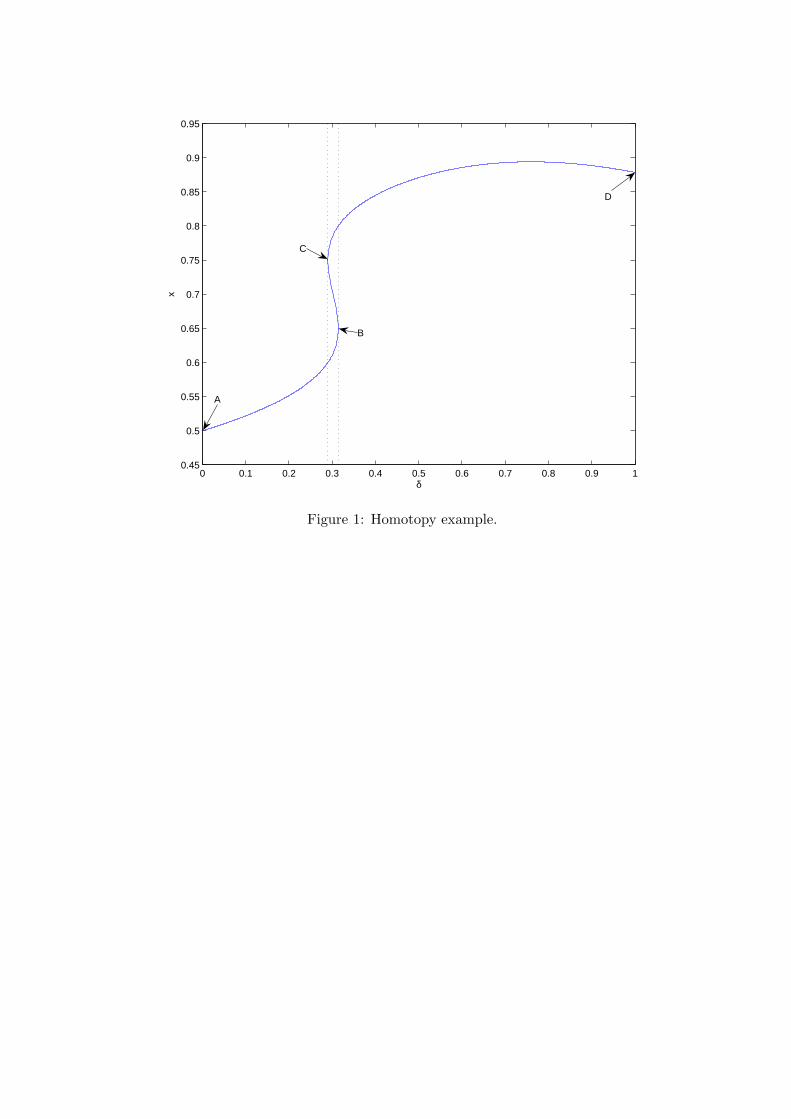
0 0.1 0.2 0.3 0.4 0.5 0.6 0.7 0.8 0.9 10.45

0.5

0.55

0.6

0.65

0.7

0.75

0.8

0.85

0.9

0.95

δ

x

A

B

C

D

Figure 1: Homotopy example.

0 0.01 0.03 0.05 0.1 0.2

0.1

0.2

0.3

0.4

0.5

0.6

0.7

0.8

0.9

1

δ

ρ

1 3 5 7 9

Figure 2: Number of equilibria.

0 0.03 0.1 0.3 10.5

0.51

0.55

0.7

1

δ

H∞

, H∧

ρ = 0.95

0 0.03 0.1 0.3 10.5

0.51

0.55

0.7

1

δ

H∞

, H∧

ρ = 0.75

0 0.03 0.1 0.3 10.5

0.51

0.55

0.7

1

δ

H∞

, H∧

ρ = 0.85

0 0.03 0.1 0.3 10.5

0.51

0.55

0.7

1

δ

H∞

, H∧

ρ = 0.65

0 0.03 0.1 0.3 10.5

0.51

0.55

0.7

1

δ

H∞

, H∧

ρ = 0.55

0 0.03 0.1 0.3 10.5

0.51

0.55

0.7

1

δ

H∞

, H∧

ρ = 0.15

0 0.03 0.1 0.3 10.5

0.51

0.55

0.7

1

δ

H∞

, H∧

ρ = 0.35

0 0.03 0.1 0.3 10.5

0.51

0.55

0.7

1

δ

H∞

, H∧

ρ = 0.05

Figure 3: Limiting expected Herfindahl index H∞ (solid line) and maximum expectedHerfindahl index H∧ (dashed line).

15

1015

2025

30

15

1015

2025

30

02468

1012

e1

Flat Eqbm. without Well (ρ=0.85, δ=0)

e2

p* (e1,e

2)

15

1015

2025

30

15

1015

2025

30

02468

1012

e1

Flat Eqbm. with Well (ρ=0.85, δ=0.0275)

e2

p* (e1,e

2)

15

1015

2025

30

15

1015

2025

30

02468

1012

e1

Trenchy Eqbm. (ρ=0.85, δ=0.0275)

e2

p* (e1,e

2)

15

1015

2025

30

15

1015

2025

30

02468

1012

e1

Extra−trenchy Eqbm. (ρ=0.85, δ=0.08)

e2

p* (e1,e

2)

Figure 4: Policy function p∗(e1, e2). Marginal cost c(e1) (solid line in e2 = 30-plane).

1 5 10 15 20 25 301

510

1520

2530

0

0.05

0.1

0.15

e1

Flat Eqbm. without Well (ρ=0.85, δ=0)

e2

µ8 (e1,e

2)

1 5 10 15 20 25 301

510

1520

2530

0

0.05

0.1

e1

Flat Eqbm. with Well (ρ=0.85, δ=0.0275)

e2

µ8 (e1,e

2)

1 5 10 15 20 25 301

510

1520

2530

0

0.05

0.1

e1

Trenchy Eqbm. (ρ=0.85, δ=0.0275)

e2

µ8 (e1,e

2)

1 5 10 15 20 25 301

510

1520

2530

0

0.05

0.1

0.15

e1

Extra−trenchy Eqbm. (ρ=0.85, δ=0.08)

e2

µ8 (e1,e

2)

Figure 5: Transient distribution over states in period 8 given initial state (1, 1).

1 5 10 15 20 25 301

510

1520

2530

0

0.02

0.04

0.06

0.08

e1

Flat Eqbm. without Well (ρ=0.85, δ=0)

e2

µ32(e

1,e2)

1 5 10 15 20 25 301

510

1520

2530

0

0.005

0.01

0.015

0.02

e1

Flat Eqbm. with Well (ρ=0.85, δ=0.0275)

e2

µ32(e

1,e2)

1 5 10 15 20 25 301

510

1520

2530

0

0.01

0.02

0.03

0.04

e1

Trenchy Eqbm. (ρ=0.85, δ=0.0275)

e2

µ32(e

1,e2)

1 5 10 15 20 25 301

510

1520

2530

0

0.02

0.04

e1

Extra−trenchy Eqbm. (ρ=0.85, δ=0.08)

e2

µ32(e

1,e2)

Figure 6: Transient distribution over states in period 32 given initial state (1, 1).

1 5 10 15 20 25 301

510

1520

2530

0

0.5

1

e1

Flat Eqbm. without Well (ρ=0.85, δ=0)

e2

µ∞(e

1,e2)

1 5 10 15 20 25 301

510

1520

2530

0

0.005

0.01

0.015

0.02

e1

Flat Eqbm. with Well (ρ=0.85, δ=0.0275)

e2

µ∞(e

1,e2)

1 5 10 15 20 25 301

510

1520

2530

0

0.005

0.01

0.015

0.02

e1

Trenchy Eqbm. (ρ=0.85, δ=0.0275)

e2

µ∞(e

1,e2)

1 5 10 15 20 25 301

510

1520

2530

0

0.01

0.02

0.03

0.04

e1

Extra−trenchy Eqbm. (ρ=0.85, δ=0.08)

e2

µ∞(e

1,e2)

Figure 7: Limiting distribution over states.

0 0.01 0.03 0.05 0.1 0.2 1

0.1

0.2

0.3

0.4

0.5

0.6

0.7

0.8

0.9

1

δ

ρ

0.000 0.333 0.667 1.000

Figure 8: Share of equilibria violating upper bound on equilibrium prices (Result 4).

0 0.01 0.03 0.05 0.1 0.2 1

0.1

0.2

0.3

0.4

0.5

0.6

0.7

0.8

0.9

1

δ

ρ

0.000 0.333 0.667 1.000

Figure 9: Share of equilibria violating lower bound on equilibrium prices (parts (i) and (ii)of Proposition 3).

1 m e−1 e M1

m

e−1

e

M

e1

e 2

δ=0 → static Nash pricesδ>0 → price aggressively

leader underprices follower

price aggressively

Figure 10: Diagonal trench.

0 0.01 0.03 0.05 0.1 0.2 1

0.1

0.2

0.3

0.4

0.5

0.6

0.7

0.8

0.9

1

δ

ρ

0.000 0.333 0.667 0.800 1.000

0 0.01 0.03 0.05 0.1 0.2 1

0.1

0.2

0.3

0.4

0.5

0.6

0.7

0.8

0.9

1

δ

ρ

0.000 0.333 0.667 0.800 1.000

Figure 11: Share of equilibria violating IID (part (i) of Result 7, upper panel) and share ofequilibria violating ID (part (ii) of Result 7, lower panel).

15

1015

2025

30

15

1015

2025

30

02468

1012

e1

Policy Function

e2

p* (e1,e

2)

1 5 10 15 20 25 301

510

1520

2530

0

0.05

0.1

e1

Transient Distribution (T=8)

e2

µ8 (e1,e

2)

1 5 10 15 20 25 301

510

1520

2530

0

0.005

0.01

0.015

0.02

e1

Transient Distribution (T=32)

e2

µ32(e

1,e2)

1 5 10 15 20 25 301

510

1520

2530

0

0.005

0.01

0.015

0.02

e1

Limiting Distribution

e2

µ∞(e

1,e2)

Figure 12: Bottomless learning. Policy function p∗(e1, e2). Marginal cost c(e1) (solid linein e2 = 30-plane) (upper left panel). Transient distribution over states in period 8 and32 given initial state (1, 1) (upper right and lower left panels). Limiting distribution overstates (lower right panel). Plateau equilibrium (ρ = 0.9, δ = 0.04).