Learning curves for drug response prediction in cancer cell linesAlexander Partin1,2* , Thomas Brettin2,3, Yvonne A. Evrard4, Yitan Zhu1,2, Hyunseung Yoo1,2, Fangfang Xia1,2, Songhao Jiang7, Austin Clyde1,7, Maulik Shukla1,2, Michael Fonstein5, James H. Doroshow6 and Rick L. Stevens3,7

Abstract

Background: Motivated by the size and availability of cell line drug sensitivity data, researchers have been developing machine learning (ML) models for predicting drug response to advance cancer treatment. As drug sensitivity studies continue generating drug response data, a common question is whether the generalization performance of existing prediction models can be further improved with more training data.

Methods: We utilize empirical learning curves for evaluating and comparing the data scaling properties of two neural networks (NNs) and two gradient boosting decision tree (GBDT) models trained on four cell line drug screening datasets. The learning curves are accurately fitted to a power law model, providing a framework for assessing the data scaling behavior of these models.

Results: The curves demonstrate that no single model dominates in terms of predic-tion performance across all datasets and training sizes, thus suggesting that the actual shape of these curves depends on the unique pair of an ML model and a dataset. The multi-input NN (mNN), in which gene expressions of cancer cells and molecular drug descriptors are input into separate subnetworks, outperforms a single-input NN (sNN), where the cell and drug features are concatenated for the input layer. In contrast, a GBDT with hyperparameter tuning exhibits superior performance as compared with both NNs at the lower range of training set sizes for two of the tested datasets, whereas the mNN consistently performs better at the higher range of training sizes. Moreover, the trajectory of the curves suggests that increasing the sample size is expected to further improve prediction scores of both NNs. These observations demonstrate the benefit of using learning curves to evaluate prediction models, providing a broader perspective on the overall data scaling characteristics.

Conclusions: A fitted power law learning curve provides a forward-looking metric for analyzing prediction performance and can serve as a co-design tool to guide experi-mental biologists and computational scientists in the design of future experiments in prospective research studies.

Keywords: Learning curve, Power law, Drug response prediction, Cell line, Deep learning, Machine learning

Open Access

© The Author(s), 2021. Open Access This article is licensed under a Creative Commons Attribution 4.0 International License, which permits use, sharing, adaptation, distribution and reproduction in any medium or format, as long as you give appropriate credit to the original author(s) and the source, provide a link to the Creative Commons licence, and indicate if changes were made. The images or other third party material in this article are included in the article’s Creative Commons licence, unless indicated otherwise in a credit line to the mate-rial. If material is not included in the article’s Creative Commons licence and your intended use is not permitted by statutory regulation or exceeds the permitted use, you will need to obtain permission directly from the copyright holder. To view a copy of this licence, visit http:// creat iveco mmons. org/ licen ses/ by/4. 0/. The Creative Commons Public Domain Dedication waiver (http:// creat iveco mmons. org/ publi cdoma in/ zero/1. 0/) applies to the data made available in this article, unless otherwise stated in a credit line to the data.

RESEARCH ARTICLE

Partin et al. BMC Bioinformatics (2021) 22:252 https://doi.org/10.1186/s12859-021-04163-y

*Correspondence: apartin@anl.gov 1 Division of Data Science and Learning, Argonne National Laboratory, Lemont, IL, USAFull list of author information is available at the end of the article

Page 2 of 18Partin et al. BMC Bioinformatics (2021) 22:252

BackgroundHuman cancer cell lines remain a primary cancer-mimicking environment in a labora-tory setting for understanding the molecular biology of this complex disease [1–3]. In the search for anticancer treatments, in  vitro drug sensitivity assays serve as a stand-ard, high-throughput experimental platform for measuring the response of cancer cells to drug treatments. The standardized protocols of sensitivity assays, along with rapid improvement of technologies for genomic profiling, have led researchers to generate large pharmacogenomic drug response datasets for anticancer drug discovery [4–6]. Considering the scale and diversity of tumors and compounds in these datasets, machine learning (ML) techniques have become a natural fit for analytically predicting the response of cell lines to drug treatments. By maneuvering through a landscape of com-putational approaches and numerical representations of tumors and drugs, research-ers strive to develop highly predictive ML drug response models [7–9]. Demonstrating the accuracy and robustness of prediction models is essential in order to identify their potential utility for clinical applications in cancer treatment including precision oncol-ogy and drug repurposing.

In ML-driven cancer research, a common question is whether existing predictive mod-els can be further improved with more training data. Given recent advances in artificial neural networks (NNs), deep learning (DL) methods have become a favorite approach across a variety of scientific disciplines for discovering hidden patterns in large volumes of complex data. This trend is also observed in medical applications, including the pre-diction of drug response in cancer cell lines [10–14]. Regardless of the learning algo-rithm, supervised learning models are expected to improve generalization performance with increasing amounts of high-quality labeled data. Generalization performance refers to the aggregated accuracy of model predictions on a set of unseen data samples. Ana-lytically estimating the learning capacity of models is a challenging task. Alternatively, given a dataset and a learning algorithm, the projected improvement of predictions with increasing number of training samples can be empirically estimated by using learning curves.

A learning curve is a plot of the generalization performance of a supervised learning model as a function of training set size (Fig. 1). These curves have been explored as an efficient method for modeling the power law relationship, s(m) ∝ amb , between the gen-eralization score s (such as generalization error or accuracy) and the number of training samples m, where a and b are two parameters of the power law model. The power law characteristics of learning curves can provide insights into the data scaling behavior of drug response prediction models, which otherwise could not be investigated by merely analyzing single-value performance measures obtained with the full training set size.

A main bottleneck of utilizing learning curves, however, is often the limited availability of sufficient computational resources for performing the analysis. Particularly challeng-ing is analysis with DL models and large datasets because of the large computational cost. While learning curves have been explored in a variety of small-scale applications with classical ML [15–18], only a few recent studies have applied DL methods to large benchmark datasets in vision and text applications [19–21]. To the best of our knowl-edge, learning curves of drug response prediction models have not been previously explored.

Page 3 of 18Partin et al. BMC Bioinformatics (2021) 22:252

In this paper, we utilize learning curves to evaluate the data scaling properties of drug response prediction models in cancer cell lines. The primary objective of fitting a power law expression to raw data is twofold: (1) efficient and accurate estimation of prediction performance with a larger, not yet available or computationally prohibitive dataset, and (2) fair and systematic comparison of prediction models across various learning algo-rithms and datasets. To that end, we perform a systematic comparison between classical ML and DL models, implemented with large pharmacogenomic drug response datasets. To accomplish these objectives, we develop an efficient computational workflow, lever-aging high-performance computing (HPC) resources to conduct the large-scale analysis. We use this workflow for generating learning curve data with gradient boosting decision tree (GBDT) models and NNs, where each model is trained on four large drug response datasets of cancer cell lines. To assess the data scaling trajectory of each dataset-model pair, the power law expression is fitted to the raw learning curve data to generate a learn-ing curve and uncertainty estimates of the curve. We apply this methodology to analyze sixteen dataset-model combinations.

Learning curvesTheoretical [22, 23] and empirical [15, 20, 21] studies demonstrate that learning curves of predictive models are characterized by a power law relationship between the training set size m and the generalization score s,

where β = (a, b, c) is the set of the power law parameters. The parameters in β deter-mine the shape of the curve and typically vary for individual combinations of learning algorithm, prediction task, and data.

An empirical learning curve often exhibits three primary learning regions: small-data, power law, and irreducible error [20]. Figure 1 provides a glimpse into the experimental results discussed later. All three learning regions of the power law expression in Eq. (1) are distinguishable on the log-log plot in Fig. 1b. Alternatively, the linear scale represen-tation in Fig. 1a visually obscures these learning trends.

(1)s(m) = amb + c,

Fig. 1 Learning curve plotted on a linear scale in (a) and on a log scale in (b). The vertical axis is the generalization score in terms of the mean absolute error of model predictions. Each data point is the averaged prediction error, computed on a test set, of a gradient boosting decision tree (GBDT) that was trained on a subset of training samples of the GDSC1 dataset

Page 4 of 18Partin et al. BMC Bioinformatics (2021) 22:252

The small-data region is attributed to the lack of an appropriate amount of training samples for learning a sufficiently generalizable model. This region produces models that perform as good as, or slightly better than, random (or best) guessing and therefore is commonly known as the region of random guess [20, 21]. On a log-log plot, the random guessing is characterized primarily by a horizontal flat region, followed by a transition to the power law region.

From random guessing, the curve transitions to the power law region described by the amb term. In this region, the curve maintains a steady trajectory, as shown by the approximately constant slope on the log-log plot in Fig.  1b. The parameter b, ranging between 0 < |b| < 1 , is the scaling exponent and determines the steepness of the curve in the power law region [16, 20, 24].

As the training size increases, the model starts to exhaust its learning capacity, gradu-ally approaching a plateau, known as the irreducible asymptotic error [16, 20, 21]. The constant term c in Eq. (1) accounts for a smooth transition from the power law region into this plateau. When this convergence region becomes apparent in the plot, it implies that the model is not expected to significantly improve with more training data, pro-viding researchers with valuable information for future directions in their attempts to improve model predictions.

Learning curves provide intuitive insight into the data scaling behavior of prediction performance, as opposed to single-value performance measures obtained with the entire set of training samples. The shape of these curves facilitates comparison between ML models by illustrating a global trajectory of model improvement. Thus, learning curves can be utilized for quantifying the learning capacity of prediction models with increas-ing amounts of training data.

MethodsThis section describes the drug response datasets, learning algorithms, training proce-dures, and methodology for generating and fitting learning curves.

Drug response datasets

The four datasets used for the experiments are listed in Table 1. The data comes from public repositories of drug sensitivity studies: the Genomics of Drug Sensitivity in Can-cer project, which includes GDSC1 and GDSC2 datasets [4]; the Cancer Therapeutics Response Portal (CTRP v2) [5]; and the NCI-60 Human Tumor Cell Lines Screen (NCI-60) [6].

In drug sensitivity data, the drug response of a cancer cell line to a drug treatment is measured by the percentage of viable cells at multiple drug doses. A three-parameter

Table 1 Datasets used for training ML models and generating learning curves

Dataset Responses Cell Lines Drugs

GDSC1 144,832 634 311

GDSC2 98,032 554 174

CTRP 254,566 812 495

NCI-60 750,000 59 47,541

Page 5 of 18Partin et al. BMC Bioinformatics (2021) 22:252

Hill–Slope model was used to fit the dose response curve for each cell-drug pair. To retain high-quality response data, we removed samples in which the R2 of the dose response curve fit was lower than 0.3. The fitted curve was used to calculate the area under the curve (AUC) over a dose range of [10−10 M, 10−4M]. The AUC value was then normalized by the dose range to take a value between 0 and 1. We note that lower AUC values indicate higher growth inhibition (i.e., stronger response to drug treatment). Fig-ure 2 shows the histograms of the response values.

The NCI-60 dataset originally included more than 3 million samples, where a sample refers to a drug response of a cell-drug pair. We randomly selected 750,000 samples from the full NCI-60 collection for our analysis. For the GDSC1, GDSC2, and CTRP datasets, we collected all the available samples for which we were able to retrieve or calculate fea-ture representations of cells and drugs.

Representation of cell lines

A variety of genomic representations of cancer cells have been used as input features for drug response prediction [25–27]. A number of studies have shown, however, that gene expression exhibits a superior predictive power for modeling drug response in cancer cells [7, 25, 28]. For our analysis, we used gene expression data generated by the RNA-Seq technology. The expression data was collected from two public data repositories: NCI-60 and Cancer Cell Line Encyclopedia (CCLE). For the cells in the NCI-60 data-set in Table 1, the RNA-Seq was retrieved from the NCI-60 repository. For the GDSC1, GDSC2, and CTRP datasets, the RNA-Seq was retrieved from the NCI-60 and CCLE repositories by matching the cell line names across the databases. Drug response sam-ples for which the cell gene expressions were not available in CCLE or NCI-60 were excluded from the datasets.

Fig. 2 Histograms of dose-independent drug response (AUC) values of the four datasets listed in Table 1

Page 6 of 18Partin et al. BMC Bioinformatics (2021) 22:252

The retrieved RNA-Seq data, provided in FPKM (fragments per kilobase million) values, was transformed into TPM (transcripts per kilobase million) values. Instead of using expressions of more than 20,000 available genes for modeling drug response, we used the expressions of 976 landmark genes as identified by the Library of Integrated Network-Based Cellular Signatures (LINCS) project [29]. The LINCS gene set has been shown to comprehensively characterize transcriptomic changes under various chemical and genetic perturbations [29].

Representation of drugs

Classical ML algorithms such as GBDT ignore the arrangement of features in datasets while utilizing the feature values only. Since we want to compare the learning curves of classical ML and DL models, we used molecular descriptors as drug representa-tions in which the ordering of features is not intended to carry meaningful information. The descriptors were generated by using the Mordred software package [30]. The full descriptor set comprises 1,826 features, including both 2-D and 3-D molecular structure descriptors. Since most of the 3-D descriptors resulted in invalid (NaN) values for the majority of compounds, we retained only the 2-D descriptors, providing a total of 1,613 drug features.

Machine learning for drug response prediction

This section first presents the formulation of drug response prediction as a super-vised learning problem and then describes the learning algorithms and model training procedures.

Drug response prediction as a supervised learning task

Consider the following definitions for a supervised learning problem of drug response prediction. Given a training set T with M samples, T = {xi, yi}

Mi=1 , xi is a feature vector

for cell-drug pair i, and yi is the corresponding dose-independent drug response. The prediction task is to learn a mapping function f : RC+D → R , where C and D are the number of gene expressions and drug descriptors, respectively. Drug response datasets comprise a unique set of cell-drug pairs, X = [Xc Xd] = {[xc,i xd,i]}

Mi=1 , where xc,i and

xd,i are, respectively, the cell and drug feature vectors of the ith pair. The algorithm learns the mapping function (i.e., prediction model) by minimizing a regression loss function, which in our analysis is the mean squared error of prediction outcomes.

Note that each cancer cell line was screened against multiple drugs and, vice versa, each drug was tested on multiple cell lines. Thus, although each cell-drug combination is unique in the training set T, the feature vectors of individual cells, xc , and drugs, xd , appear multiple times in T. The analysis of how this redundancy in feature space affects prediction models and learning curves is beyond the scope of this paper and provides a topic for further investigation.

Machine learning models and training procedures

NNs can be designed to enhance learning from a particular feature type of cell or drug [11, 31]. In such models, the prediction performance depends on the availability, quality,

Page 7 of 18Partin et al. BMC Bioinformatics (2021) 22:252

and diversity of that specific feature type in a training set. In contrast, our primary objective is to gain insight into the overall prediction improvement with an increasing number of training samples. Thus, we refrained from using architectures that focus on learning from specific feature types of cells or drugs.

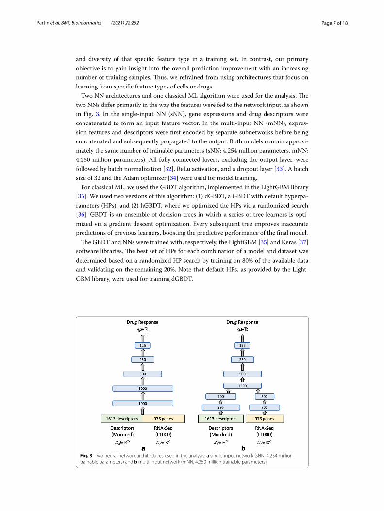
Two NN architectures and one classical ML algorithm were used for the analysis. The two NNs differ primarily in the way the features were fed to the network input, as shown in Fig.  3. In the single-input NN (sNN), gene expressions and drug descriptors were concatenated to form an input feature vector. In the multi-input NN (mNN), expres-sion features and descriptors were first encoded by separate subnetworks before being concatenated and subsequently propagated to the output. Both models contain approxi-mately the same number of trainable parameters (sNN: 4.254 million parameters, mNN: 4.250 million parameters). All fully connected layers, excluding the output layer, were followed by batch normalization [32], ReLu activation, and a dropout layer [33]. A batch size of 32 and the Adam optimizer [34] were used for model training.

For classical ML, we used the GBDT algorithm, implemented in the LightGBM library [35]. We used two versions of this algorithm: (1) dGBDT, a GBDT with default hyperpa-rameters (HPs), and (2) hGBDT, where we optimized the HPs via a randomized search [36]. GBDT is an ensemble of decision trees in which a series of tree learners is opti-mized via a gradient descent optimization. Every subsequent tree improves inaccurate predictions of previous learners, boosting the predictive performance of the final model.

The GBDT and NNs were trained with, respectively, the LightGBM [35] and Keras [37] software libraries. The best set of HPs for each combination of a model and dataset was determined based on a randomized HP search by training on 80% of the available data and validating on the remaining 20%. Note that default HPs, as provided by the Light-GBM library, were used for training dGBDT.

Fig. 3 Two neural network architectures used in the analysis: a single-input network (sNN, 4.254 million trainable parameters) and b multi-input network (mNN, 4.250 million trainable parameters)

Page 8 of 18Partin et al. BMC Bioinformatics (2021) 22:252

To mitigate overfitting, we used the early stopping functionality, available in both LightGBM and Keras. With early stopping, the model training procedure is terminated if the prediction performance on a validation set has not improved for a specified num-ber of training iterations. We set the early stopping parameter to 25 epochs for the NNs and 50 boosting rounds for GBDT models. To guarantee convergence of NNs, we used a sufficiently large number of 500 epochs to ensure that the early stopping function was triggered.

Workflow for generating and fitting learning curves

This section lays out the methodology for generating learning curve data and fitting a power law model. A schematic of the workflow is illustrated in Fig. 4.

Data partitioning

A dataset D is randomly shuffled and split into three disjoint sets: training T, validation V, and test E. Shuffling D before generating the splits increases the likelihood that the three partitions exhibit a similar distribution of drug responses. A total of N = 20 com-binations, {T ,V ,E}Nn=1 , were generated by shuffling D with different random seeds. Each set {T ,V ,E} maintains the same size proportion of (0.8, 0.1, 0.1) as a fraction of the total number of samples |D|.

Fig. 4 Workflow for generating learning curve data, LC, for a single split of a dataset. A single dataset split includes three sample sets: training T, validation V, and test E

Page 9 of 18Partin et al. BMC Bioinformatics (2021) 22:252

For each of the N splits, we form a set of K training subsets, {Tk}Kk=1

, of increasing sizes mk−1 < mk , where mk is the sample size of Tk . The samples are sequentially pulled from T to form each subset Tk , as illustrated in Fig. 4. This process ensures that each subset contains all the training samples from the immediately preceding subset such that Tk−1 ⊆ Tk . The inclusion of the entire subset Tk−1 in Tk mimics the temporal evolution of a research study where new samples are added to an already available dataset. Note that shuffling D at the first step of this data partitioning workflow is essential to enable the sequential sampling from T while eliminating potential biases associated with the original ordering of samples in D.

Generating learning curve data

Once the N data splits and the K training subsets for each split are generated, a total of N × K prediction models are trained. In order to support early stopping, the training is terminated if the generalization performance on the validation set V has not improved over a predefined number of training iterations. Upon training completion, the model predicts the response for each cell-drug pair in the test set E. Note that within a given data split n, all K models use the same validation and test sets (V and E) irrespective of mk.

The predictions on test set E are aggregated into a single score, snk , by com-puting the mean absolute error of predictions, where snk is the generalization error for a subset of size mk of split n. As a result, the raw learning curve data, LCraw = {snk }, k = 1, . . . ,K ; n = 1, . . . ,N , is produced. The total number of models trained for each combination of a dataset and a model depends on the values of N and K. For most dataset-model pairs, we trained K = 10 models per split, resulting in a total of 200 models (200 raw LC error scores).

There is no sequential dependency in terms of model training with different subsets and data splits for generating the raw LC data. Thus, the proposed workflow enables the trainings to be distributed across multiple processors. The workflow was parallelized on appropriate platforms depending on the ML software framework. The NNs were trained on the Summit HPC, while the GBDT models were trained on a CPU cluster.

Curve fitting

The raw learning curve data, LCraw , contains N × K error scores that were obtained for N data splits and K training sizes. The power law expression in Eq. (1) primarily accounts for error scores that span the power law ( amb term) and plateau (constant c) regions, while mostly excludes the region of small-data. Thus, an inadequate choice of data points can lead to a bad fit.

As a first step in producing a reliable fit, we visually identified error scores in the small-data region and excluded them from LCraw , as shown in Fig. 5a, where mkmin is the smallest sample size that was considered for further analysis. The remaining scores were considered next for fitting the power law expression, s(m) = amb + c , with β = (a, b, c) being the parameters to be estimated. We used the weighted version of the least-squares fit to prioritize the contribution of larger subsets (i.e., larger weights, αk , were assigned to larger values of mk ) which essentially reduces the effect of small train-ing subsets that are in close proximity with random guessing. Specifically, each score

Page 10 of 18Partin et al. BMC Bioinformatics (2021) 22:252

was assigned a weight that is normalized by the sample size, αk = mk/mK [18, 38]. The parameter estimates β were obtained for each split n by fitting the remaining scores with a weighted nonlinear least-squares minimization method as described in [38], produc-ing N combinations of parameter estimates, {βn}Nn=1 , where βn are the estimated power law parameters for split n. For each n, we used {mk}

Kk=kmin

to compute a set of power law values, sn(mk) = s(mk; βn) , based on Eq. 1. The N sets of all the computed power law values, y(mk) = {sn(mk)}

Nn=1 , as well as the corresponding median (i.e., the 0.5th quan-

tile) values computed across the N sets, q0.5(mk) � y(mk) = {sn(mk)}Kk=kmin

, are shown as gray and black dots, respectively, in Fig. 5b. In a similar manner of computing y(mk) , we computed the 0.1th quantile, q0.1(mk) , and 0.9th quantile, q0.9(mk) . Finally, we fit the power law to y(mk) , q0.1(mk) , and q0.9(mk) , which represent, respectively, the error score estimates for a given dataset-model combination (black curve), and the corresponding lower and upper variability estimates of the fit (shaded region bounded by the blue and green curves).

We used the MAEfit and R2fit as the goodness-of-fit measures. The MAEfit is the mean

of absolute value of residuals between the values representing the error estimates (black dots) and the values representing the fit (black curve), where smaller values of MAEfit indicate a closer fit. These measures have been shown as appropriate metrics for evaluat-ing the quality of the power law fit [17, 18].

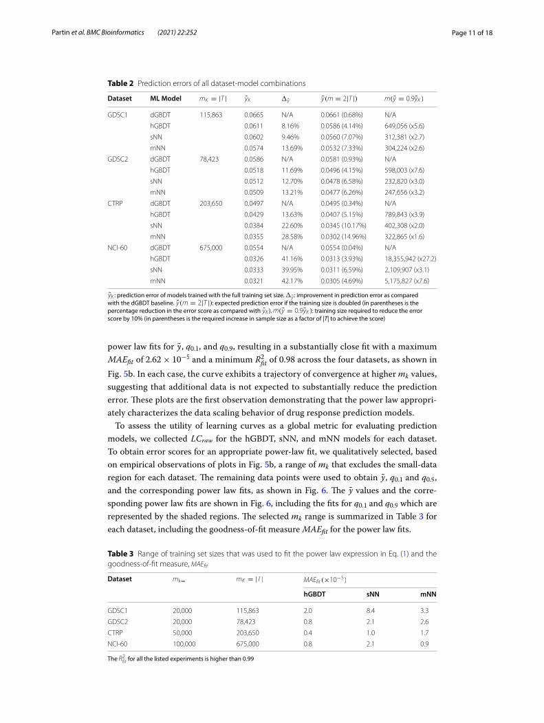
ResultsA single experiment refers to the workflow of generating LCraw and fitting the power law expression in Eq. (1) to y , q0.1 , and q0.9 , for a pair of a dataset and an ML model. Pairing all the possible combinations results in a total of sixteen experiments. The prediction error scores of models trained with the full training set, yK = y(m = mK ) , are listed in Table 2. The dGBDT serves as the baseline model in this comparison and is used to cal-culate the reduction in error score of other models with

where α is the evaluated ML model. All models yield lower yK as compared with dGBDT, exhibiting an improvement of 8% up to 42% across the datasets. While these results were expected, the observed improvements render dGBDT as an inadequate baseline for drug response prediction.

Because of the large difference in performance between dGBDT and the other mod-els, we analyze the learning curves of dGBDT separately in Fig. 5. Since LightGBM is highly parallelizable and allows faster model convergence as compared with NNs, we train 1,000 dGBDT models ( N = 20 , K = 50 ) with each of the four datasets, as shown in Fig. 5a. Note that the three regions of the learning curve are apparent in each plot.

The small-data region especially stands out because of the large spread of scores on the vertical axis. The power law region follows next and can be identified as the linear region on the log−log plot. The curve then starts to converge and progresses to the range of irreducible error. We visually identified the data points within the small-data region and excluded them from LCraw . The remaining points were used to obtain the

(2)�y(α) = 100 ·yK (α)− yK (dGBDT )

yK (dGBDT ),

Page 11 of 18Partin et al. BMC Bioinformatics (2021) 22:252

power law fits for y , q0.1 , and q0.9 , resulting in a substantially close fit with a maximum MAEfit of 2.62× 10−5 and a minimum R2

fit of 0.98 across the four datasets, as shown in Fig. 5b. In each case, the curve exhibits a trajectory of convergence at higher mk values, suggesting that additional data is not expected to substantially reduce the prediction error. These plots are the first observation demonstrating that the power law appropri-ately characterizes the data scaling behavior of drug response prediction models.

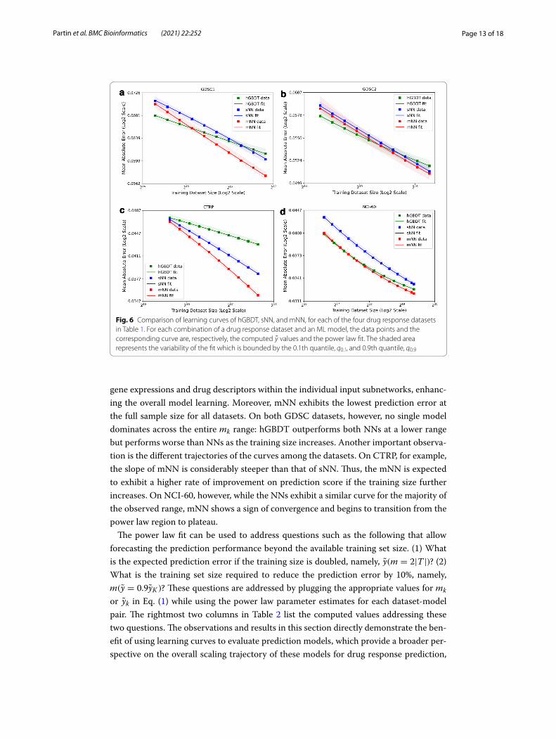
To assess the utility of learning curves as a global metric for evaluating prediction models, we collected LCraw for the hGBDT, sNN, and mNN models for each dataset. To obtain error scores for an appropriate power-law fit, we qualitatively selected, based on empirical observations of plots in Fig. 5b, a range of mk that excludes the small-data region for each dataset. The remaining data points were used to obtain y , q0.1 and q0.9 , and the corresponding power law fits, as shown in Fig. 6. The y values and the corre-sponding power law fits are shown in Fig. 6, including the fits for q0.1 and q0.9 which are represented by the shaded regions. The selected mk range is summarized in Table 3 for each dataset, including the goodness-of-fit measure MAEfit for the power law fits.

Table 2 Prediction errors of all dataset-model combinations

yK : prediction error of models trained with the full training set size. �y : improvement in prediction error as compared with the dGBDT baseline. y(m = 2|T |) : expected prediction error if the training size is doubled (in parentheses is the percentage reduction in the error score as compared with yK ). m(y = 0.9yK ) : training size required to reduce the error score by 10% (in parentheses is the required increase in sample size as a factor of |T| to achieve the score)

Dataset ML Model mK = |T | yK �y y(m = 2|T |) m(y = 0.9yK )

GDSC1 dGBDT 115,863 0.0665 N/A 0.0661 (0.68%) N/A

hGBDT 0.0611 8.16% 0.0586 (4.14%) 649,056 (x5.6)

sNN 0.0602 9.46% 0.0560 (7.07%) 312,381 (x2.7)

mNN 0.0574 13.69% 0.0532 (7.33%) 304,224 (x2.6)

GDSC2 dGBDT 78,423 0.0586 N/A 0.0581 (0.93%) N/A

hGBDT 0.0518 11.69% 0.0496 (4.15%) 598,003 (x7.6)

sNN 0.0512 12.70% 0.0478 (6.58%) 232,820 (x3.0)

mNN 0.0509 13.21% 0.0477 (6.26%) 247,656 (x3.2)

CTRP dGBDT 203,650 0.0497 N/A 0.0495 (0.34%) N/A

hGBDT 0.0429 13.63% 0.0407 (5.15%) 789,843 (x3.9)

sNN 0.0384 22.60% 0.0345 (10.17%) 402,308 (x2.0)

mNN 0.0355 28.58% 0.0302 (14.96%) 322,865 (x1.6)

NCI-60 dGBDT 675,000 0.0554 N/A 0.0554 (0.04%) N/A

hGBDT 0.0326 41.16% 0.0313 (3.93%) 18,355,942 (x27.2)

sNN 0.0333 39.95% 0.0311 (6.59%) 2,109,907 (x3.1)

mNN 0.0321 42.17% 0.0305 (4.69%) 5,175,827 (x7.6)

Table 3 Range of training set sizes that was used to fit the power law expression in Eq. (1) and the goodness-of-fit measure, MAEfit

The R2fit for all the listed experiments is higher than 0.99

Dataset mk=1 mK = |T | MAEfit(×10−5)

hGBDT sNN mNN

GDSC1 20,000 115,863 2.0 8.4 3.3

GDSC2 20,000 78,423 0.8 2.1 2.6

CTRP 50,000 203,650 0.4 1.0 1.7

NCI-60 100,000 675,000 0.8 2.1 0.9

Page 12 of 18Partin et al. BMC Bioinformatics (2021) 22:252

As Fig.  6 indicates, mNN outperforms sNN across the entire range of the explored training sizes on every dataset, albeit with the similar number of trainable parameters in these NNs. This superiority of mNN can be attributed to the separate encoding of

Fig. 5 Learning curves generated by using dGBDT for multiple data splits of each of the datasets in Table 1. a The entire set of learning curve scores, LCraw , where each data point is the mean absolute error of predictions computed on test set E as a function of the training set size mk . A subset of scores in which the sample size is above mkmin (dashed black line) was considered for curve fitting. b Three curves were generated to represent the fit: q0.1 (blue curve) and q0.9 (green curve) representing the variability of the fit, and y (black curve) representing the learning curve fit

Page 13 of 18Partin et al. BMC Bioinformatics (2021) 22:252

gene expressions and drug descriptors within the individual input subnetworks, enhanc-ing the overall model learning. Moreover, mNN exhibits the lowest prediction error at the full sample size for all datasets. On both GDSC datasets, however, no single model dominates across the entire mk range: hGBDT outperforms both NNs at a lower range but performs worse than NNs as the training size increases. Another important observa-tion is the different trajectories of the curves among the datasets. On CTRP, for example, the slope of mNN is considerably steeper than that of sNN. Thus, the mNN is expected to exhibit a higher rate of improvement on prediction score if the training size further increases. On NCI-60, however, while the NNs exhibit a similar curve for the majority of the observed range, mNN shows a sign of convergence and begins to transition from the power law region to plateau.

The power law fit can be used to address questions such as the following that allow forecasting the prediction performance beyond the available training set size. (1) What is the expected prediction error if the training size is doubled, namely, y(m = 2|T |) ? (2) What is the training set size required to reduce the prediction error by 10%, namely, m(y = 0.9yK ) ? These questions are addressed by plugging the appropriate values for mk or yk in Eq. (1) while using the power law parameter estimates for each dataset-model pair. The rightmost two columns in Table 2 list the computed values addressing these two questions. The observations and results in this section directly demonstrate the ben-efit of using learning curves to evaluate prediction models, which provide a broader per-spective on the overall scaling trajectory of these models for drug response prediction,

Fig. 6 Comparison of learning curves of hGBDT, sNN, and mNN, for each of the four drug response datasets in Table 1. For each combination of a drug response dataset and an ML model, the data points and the corresponding curve are, respectively, the computed y values and the power law fit. The shaded area represents the variability of the fit which is bounded by the 0.1th quantile, q0.1 , and 0.9th quantile, q0.9

Page 14 of 18Partin et al. BMC Bioinformatics (2021) 22:252

and the utility of the power-law fits for addressing important questions in prospective research.

DiscussionThe analysis across sixteen experiments (with four datasets and four models) dem-onstrates that no single model dominates in terms of prediction performance across all datasets and training sizes. This result supports the assumption that the actual shape of learning curves depends on both the dataset and the model. For example, hGBDT exhibits lower error scores for a lower range of training sizes on two datasets, as shown in Fig.  6a, b. Alternatively, mNN outperforms all the investigated models (dGBDT, hGBDT, sNN) across all datasets for sufficiently large training sizes. Moreo-ver, both NNs maintain data scaling properties that are characterized by the power law region, demonstrating a promising trajectory of further improvement. These observations indicate that the power law fits can be used to project the expected error score beyond the available training size or, alternatively, calculate the sample size required to achieve a specific performance. These uses of learning curves can aid in collaboration between experimental biologists and computational scientists to shape a global vision of how predictive models can be further improved. This valuable per-spective can guide the process of new data generation, either through lab experiments or synthetically, via simulations or resampling methods.

One should be cautious, however, in generalizing the data scaling characteristics when building prediction models with subsets of the investigated datasets or modified architectures of sNN or mNN. In this study, we explored a general case where both cell and drug features predict the drug response. Alternatively, models that focus on a specific cancer type are usually trained by using an appropriate subset of cell lines of a much smaller sample size. Moreover, to mitigate overfitting with the reduced sample size, researchers may choose to limit the feature space by using the drug features only. These dataset and model changes may produce a different layout of learning curves and, therefore, different conclusions and downstream actions. We therefore recom-mend generating learning curves for every dataset-model pair that is being analyzed.

In Fig. 6b, d, we observe a moderate improvement at the full training set size with mNN as compared with hGBDT. Similarly, certain studies proposing novel DL meth-ods for drug response prediction demonstrate moderate improvement as compared with classical ML [10, 31, 39]. This is in contrast to vision and text applications where DL methods represent the state of the art [40, 41]. The complexity in design and training of models such as mNN and hGBDT is higher than that of their respective counterparts, sNN and dGBDT. While using simpler models as a demonstration vehi-cle might be tempting, such models typically result in a poor baseline for objectively evaluating the prediction performance of proposed models. Similarly, generating learning curves requires significant computational resources for performing a thor-ough analysis across multiple data splits and training sizes, as demonstrated in this study. While often time- and resource-consuming, a rigorous comparison of novel models with strong baselines is necessary for producing a significant impact and vis-ibility within the ML community.

Page 15 of 18Partin et al. BMC Bioinformatics (2021) 22:252

Contributed to the diversity and complexity of cancer pathologies, no single combi-nation of a dataset, feature type, and prediction target serves as a universal benchmark for modeling drug response. Various learning methodologies and data pre-process-ing techniques have been explored to enhance the predictive capabilities of mod-els, including multi-modal learning [11, 26], feature encoding schemes [27, 31], and transfer learning [13, 42]. The performance of these models is assessed by comparing single-value performance measures such as prediction error or accuracy against base-line models obtained at the full sample size. The lack of unified benchmarks for the drug response problem, alongside a moderate improvement in predictions as com-pared with baseline models, may cast doubt on the true potential of proposed models. In such cases, learning curves can better highlight the potential impact of models by depicting the improvement of predictions with increasing sample size. For example, assume that we analyze the performance of mNN against sNN using CTRP and NCI-60 datasets. On NCI-60, the trajectory of the curves suggests that both models are expected to converge with more training data (see Fig.  6d), whereas on CTRP, the curves portray a more favorable trajectory for mNN to potentially further improve the performance with more data (see Fig. 6c). Alternatively, when using the predic-tion performance at the full training set size, yK , both CTRP and NCI-60 exhibit a comparable superiority of mNN as compared with the sNN baseline, failing to dem-onstrate the additional dimension of comparison provided by the learning curves. To the best of our knowledge, this is the first work that proposes the use of learning curves for systematic evaluation and comparison of machine learning algorithms in drug response problem.

Similarly to learning curve studies from other scientific domains, we demonstrate that the power law in Eq. (1) closely models the data scaling for the application of drug response prediction. While other works focus primarily on a single family of ML models, we have investigated both classical ML and DL models, with a primary observation that no single model is superior to other models for all datasets and training sizes. Moreover, the extent of the three learning regions (described in Fig. 1) significantly differs among the different applications. For example, Mukherjee et  al. [16] accurately fit the power law of eight cancer-related classification tasks with DNA microarray datasets ranging between 53 and 280 samples. The prediction of drug response in cancer cell lines is presumably a more challenging task, since our models require thousands of training samples to reveal the learning regions.

While cell lines remain a primary environment for mimicking cancer, alternative biological models are being investigated as closer surrogates of human cancer. These alternatives include patient-derived xenografts (PDXs), which are cancer implants in animals, and patient-derived organoids (PDOs), which are 3-D cultures of cancer cells from patients. ML analysis with these emerging cancer environments is essential for future development of cancer treatment. At this point, however, drug response data for these biological models is scarce compared with the relatively abundant cell line screen-ing data. The scarcity of PDXs and PDOs data imposes a challenging search for suitable methods across the entire space of learning algorithms. Therefore, learning curves can serve as a useful co-design tool for comparing predictive performance of learning algo-rithms and facilitate the design of future experiments in a prospective research setting.

Page 16 of 18Partin et al. BMC Bioinformatics (2021) 22:252

ConclusionsWe demonstrate that learning curves of drug response prediction models using both classical ML and DL methods follow a power law expression. The specific trajectory of the curves depends on the dataset and the learning algorithm and therefore should be obtained empirically. While hGDBT exhibits superior performance at a lower range of training sizes, the mNN outperforms all the investigated models as the training size increases. These observations demonstrate the benefits of learning curves in mod-eling the data scaling properties of prediction models, while the proposed methodol-ogy allows to quantify the expected prediction performance across the entire range of training sizes. The power law fit can also be utilized to forecast the behavior of learning curves beyond the available training size. The fitted power law curve provides a forward-looking metric for analyzing prediction performance and can serve as a co-design tool to guide experimental biologists and computational scientists in the design of future exper-iments in prospective research studies.

AbbreviationsGBDT: Gradient boosting decision tree; dGBDT: Gradient boosting decision tree with default hyperparameters; hGBDT: Gradient boosting decision tree with hyperparameters tuning; sNN: Single-input neural network; mNN: Multi-input neu-ral network; ML: Machine learning; DL: Deep learning; MAE: Mean absolute error; LCraw: Raw learning curve data..

AcknowledgementsThe authors thank the Argonne Leadership Computing Facility (ALCF) and Oak Ridge Leadership Computing Facility (OLCF) for providing computing resources for this research.

Authors’ contributionsAP designed the study; AP, MS, AC and FX collected and pre-processed the data; AP, HY and TB conducted the experi-ments; AP, YZ, TB and RLS wrote and edited the article; AP, SJ and YZ performed data analysis; AP, TB, YAE, YZ, HY, FX, SJ, AC, MS, MF, JHD and RLS interpreted results and derived conclusions; RLS and JHD conceived the idea. All authors have read and approved the final manuscript.

FundingThis work has been supported in part by the Joint Design of Advanced Computing Solutions for Cancer (JDACS4C) program established by the U.S. Department of Energy (DOE) and the National Cancer Institute (NCI) of the National Institutes of Health. This work was performed under the auspices of the U.S. Department of Energy by Argonne National Laboratory under Contract DE-AC02-06-CH11357, Lawrence Livermore National Laboratory under Contract DE-AC52-07NA27344, Los Alamos National Laboratory under Contract DE-AC5206NA25396, and Oak Ridge National Laboratory under Contract DE-AC05-00OR22725. This project has also been funded in whole or in part with federal funds from the NCI, National Institutes of Health (NIH), under Contract No. HHSN261200800001E. The content of this publication does not necessarily reflect the views or policies of the Department of Health and Human Services, nor does mention of trade names, commercial products, or organizations imply endorsement by the U.S. Government.

Availability of data and materialsThe full code is available at https:// github. com/ adpar tin/ dr- learn ing- curves. The data that was used to train the machine learning models is available at https:// ftp. mcs. anl. gov/ pub/ pilot1/ publi catio ns/ dr- learn ing- curves/ data/.

Declarations

Ethics approval and consent to participateNot applicable.

Consent for publicationNot applicable.

Competing interestsThe authors declare that they have no competing interests.

Author details1 Division of Data Science and Learning, Argonne National Laboratory, Lemont, IL, USA. 2 University of Chicago Consor-tium for Advanced Science and Engineering, University of Chicago, Chicago, IL, USA. 3 Computing, Environment and Life Sciences, Argonne National Laboratory, Lemont, IL, USA. 4 Frederick National Laboratory for Cancer Research, Leidos Bio-medical Research Inc., Frederick, MD, USA. 5 Biosciences Division, Argonne National Laboratory, Lemont, IL, USA. 6 Division of Cancer Therapeutics and Diagnosis, National Cancer Institute, Bethesda, MD, USA. 7 Department of Computer Science, University of Chicago, Chicago, IL, USA.

Page 17 of 18Partin et al. BMC Bioinformatics (2021) 22:252

Received: 29 November 2020 Accepted: 4 May 2021

References 1. Sharma SV, Haber DA, Settleman J. Cell line-based platforms to evaluate the therapeutic efficacy of candidate

anticancer agents. Nat Rev Cancer. 2010;10:241–53. https:// doi. org/ 10. 1038/ nrc28 20. 2. Gillet J-P, Varma S, Gottesman MM. The clinical relevance of cancer cell lines. JNCI J Natl Cancer Inst.

2013;105(7):452–8. https:// doi. org/ 10. 1093/ jnci/ djt007. 3. Ben-David U, et al. Genetic and transcriptional evolution alters cancer cell line drug response. Nature. 2018;560:325–

30. https:// doi. org/ 10. 1038/ s41586- 018- 0409-3. 4. Yang W, et al. Genomics of drug sensitivity in cancer (GDSC): a resource for therapeutic biomarker discovery in

cancer cells. Nucleic Acids Res. 2013;41:955–61. https:// doi. org/ 10. 1093/ nar/ gks11 11. 5. Seashore-Ludlow B, et al. Harnessing connectivity in a large-scale small-molecule sensitivity dataset. Cancer Discov.

2015;5(11):1210–23. https:// doi. org/ 10. 1158/ 2159- 8290. CD- 15- 0235. 6. Grever MR, Schepartz SA, Chabner BA. The national cancer institute: cancer drug discovery and development pro-

gram. Semin Oncol. 1992;19:622–38. 7. Costello JC, et al. A community effort to assess and improve drug sensitivity prediction algorithms. Nat Biotechnol.

2014;32:1202–12. https:// doi. org/ 10. 1038/ nbt. 2877. 8. Niz CD, Rahman R, Zhao X, Pal R. Algorithms for drug sensitivity prediction. Algorithms. 2016;9(77):1202–12. https://

doi. org/ 10. 3390/ a9040 077. 9. Adam G, Rampášek L, Safikhani Z, Smirnov P, Haibe-Kains B, Goldenberg A. Machine learning approaches

to drug response prediction: challenges and recent progress. NPJ Precis Onc. 2020. https:// doi. org/ 10. 1038/ s41698- 020- 0122-1.

10. Rampášek L, Hidru D, Smirnov P, Haibe-Kains B, Goldenberg A. Dr.VAE: improving drug response prediction via modeling of drug perturbation effects. Bioinformatics. 2019;35(19):3743–51. https:// doi. org/ 10. 1093/ bioin forma tics/ btz158.

11. Manica M, Oskooei A, Born J, Subramanian V, Sáez-Rodríguez J, Rodríguez MM. Towards explainable anticancer com-pound sensitivity prediction via multimodal attention-based convolutional encoders. Mol Pharm. 2019;16(12):4797–806. https:// doi. org/ 10. 1021/ acs. molph armac eut. 9b005 20.

12. Bazgir O, Zhang R, Dhruba SR, Rahman R, Ghosh S, Pal R. Representation of features as images with neighborhood dependencies for compatibility with convolutional neural networks. Nat Commun. 2020;11:4391. https:// doi. org/ 10. 1038/ s41467- 020- 18197-y.

13. Zhu Y, et al. Ensemble transfer learning for the prediction of anti-cancer drug response. Sci Rep. 2020;10:18040. https:// doi. org/ 10. 1038/ s41598- 020- 74921-0.

14. Vougas K, et al. Machine learning and data mining frameworks for predicting drug response in cancer: An overview and a novel in silico screening process based on association rule mining. Pharmacol Therapeut. 2019. https:// doi. org/ 10. 1016/j. pharm thera. 2019. 107395.

15. Cortes C, Jackel LD, Solla SA, Vapnik V, Denker JS. Learning curves: Asymptotic values and rate of convergence. Adv Neural Inf Process Syst. 1994;6:327–34.

16. Mukherjee S, Tamayo P, Rogers S, Rifkin R, Engle A, Campbell C, Golub TR, Mesirov JP. Estimating dataset size require-ments for classifying DNA microarray data. J Comput Biol. 2003;10(2):119–42. https:// doi. org/ 10. 1089/ 10665 27033 21825 928.

17. Last M. Predicting and optimizing classifier utility with the power law. In: Seventh IEEE International Conference on Data Mining Workshops (ICDMW 2007), 2007; pp. 219–224. https:// doi. org/ 10. 1109/ ICDMW. 2007. 31.

18. Figueroa RL, Zeng-Treitler Q, Kandula S, Ngo LH. Predicting sample size required for classification performance. BMC Med Inform Decis Mak. 2012. https:// doi. org/ 10. 1186/ 1472- 6947- 12-8.

19. Sun C, Shrivastava A, Singh S, Gupta A. Revisiting unreasonable effectiveness of data in deep learning era. In: 2017 IEEE international conference on computer vision (ICCV), 2017; pp. 2961–2969. https:// doi. org/ 10. 1109/ ICCV. 2017. 97.

20. Hestness J et al. Deep learning scaling is predictable, empirically. arXiv e-prints; 2017. arXiv: 712. 00409. 21. Rosenfeld JS, Rosenfeld A, Belinkov Y, Shavit N. A constructive prediction of the generalization error across scales. In:

International conference on learning representations 2020. 22. Amari S-I, Fujita N, Shinomoto S. Four types of learning curves. Neural Comput. 1992;4(4):605–18. https:// doi. org/ 10.

1162/ neco. 1992.4. 4. 605. 23. Haussler D, Kearns M, Seung HS, Tishby N. Rigorous learning curve bounds from statistical mechanics. Mach Learn.

1996;25:195–236. https:// doi. org/ 10. 1023/A: 10264 99208 981. 24. Anzanello MJ, Fogliatto FS. Learning curve models and applications: Literature review and research directions. Int J

Ind Ergon. 2011;41(5):573–83. https:// doi. org/ 10. 1016/j. ergon. 2011. 05. 001. 25. Xia F, et al. Predicting tumor cell line response to drug pairs with deep learning. BMC Bioinform. 2018;19:486. https://

doi. org/ 10. 1186/ s12859- 018- 2509-3. 26. Sharifi-Noghabi H, Zolotareva O, Collins CC, Ester M. MOLI: multi-omics late integration with deep neural networks

for drug response prediction. Bioinformatics. 2019;35(14):501–9. https:// doi. org/ 10. 1093/ bioin forma tics/ btz318. 27. Zhu Y, et al. Enhanced co-expression extrapolation (coxen) gene selection method for building anti-cancer drug

response prediction models. Genes. 2020;11:1070. https:// doi. org/ 10. 3390/ genes 11091 070. 28. Jang IS, Neto EC, Guinney J, Friend SH, Margolin A. Systematic assessment of analytical methods for drug sensitivity

prediction from cancer cell line data. In: Pacific symposium on biocomputing, 2014; pp. 63–74. 29. Subramanian A, et al. A next generation connectivity map: L1000 platform and the first 1,000,000 profiles. Cell.

2017;171(6):1437–52. https:// doi. org/ 10. 1016/j. cell. 2017. 10. 049.

Page 18 of 18Partin et al. BMC Bioinformatics (2021) 22:252

• fast, convenient online submission

•

thorough peer review by experienced researchers in your field

• rapid publication on acceptance

• support for research data, including large and complex data types

•

gold Open Access which fosters wider collaboration and increased citations

maximum visibility for your research: over 100M website views per year •

At BMC, research is always in progress.

Learn more biomedcentral.com/submissions

Ready to submit your researchReady to submit your research ? Choose BMC and benefit from: ? Choose BMC and benefit from:

30. Moriwaki H, Tian Y-S, Kawashita N, Takagi T. Mordred: a molecular descriptor calculator. J Cheminform. 2018. https:// doi. org/ 10. 1186/ s13321- 018- 0258-y.

31. Cortés-Ciriano I, Bender A. Kekulescope: prediction of cancer cell line sensitivity and compound potency using convolutional neural networks trained on compound images. J Cheminform. 2019. https:// doi. org/ 10. 1186/ s13321- 019- 0364-5.

32. Ioffe S, Szegedy C. Batch normalization: accelerating deep network training by reducing internal covariate shift. In: Proceedings of the 32nd international conference on machine learning; 2015, vol. 37, pp. 448–456.

33. Srivastava N, Hinton G, Krizhevsky A, Sutskever I, Salakhutdinov R. Dropout: a simple way to prevent neural networks from overfitting. J Mach Learn Res. 2014;15(56):1929–58.

34. Kingma DP, Ba JL. Adam: a method for stochastic optimization. In: International conference on learning representa-tions (ICLR) 2015.

35. Ke G, Meng Q, Finley T, Wang T, Chen W, Ma W, Ye Q, Liu T-Y. Lightgbm: a highly efficient gradient boosting decision tree. In: Proceedings of the 31st international conference on neural information processing systems, 2017; pp. 3149–3157.

36. Bergstra J, Bengio Y. Random search for hyper-parameter optimization. J Mach Learn Res. 2012;13:281–305. 37. Chollet F et al. Keras. https:// keras. io 2015. 38. Johnson M, Anderson P, Dras M, Steedman M. Predicting accuracy on large datasets from smaller pilot data. In:

Proceedings of the 56th annual meeting of the association for computational linguistics (volume 2: short papers); 2018, pp. 450–455. https:// doi. org/ 10. 18653/ v1/ P18- 2072.

39. Chiu Y-C, Chen H-IH, Zhang T, Zhang S, Gorthi A, Wang L-J, Huang Y, Chen Y. Predicting drug response of tumors from integrated genomic profiles by deep neural networks. BMC Med Genomics. 2019;12:18. https:// doi. org/ 10. 1186/ s12920- 018- 0460-9.

40. Tan M, Pang R, Le QV. Efficientdet: scalable and efficient object detection. In: Proceedings of the IEEE/CVF confer-ence on computer vision and pattern recognition (CVPR), 2020.

41. Howard J, Ruder S. Universal language model fine-tuning for text classification. In: Proceedings of the 56th annual meeting of the association for computational linguistics (volume 1: long papers), 2018; pp. 328–339 . https:// doi. org/ 10. 18653/ v1/ P18- 1031

42. Rahman Dhruba S, Rahman R, Matlock K, Ghosh S, Pal R. Application of transfer learning for cancer drug sensitivity prediction. BMC Bioinform 2018. doi: 10.1186/s12859-018-2465-y.