Learning Decentralized Goal-based Vector · PDF fileLearning Decentralized Goal-based Vector Quantization ... From rate distortion theory, ... Learning Decentralized Goal-based Vector

Learning Decentralized Goal-basedVector Quantization

Piyush Gupta*

Department of Electrical and Computer Engineering,University of Illinois at Urbana-Champaign, Urbana, IL

Vivek S. Borkar÷

Department of Computer Science and Automation,Indian Institute of Science, Bangalore, India

This paper considers the following generalization of classical vector quan-tization: to (vector) quantize or, equivalently, to partition the domain ofa given function such that each cell in the partition satisfies a given setof topological constraints. This formulation is called decentralized goal-based vector quantization (DGVQ). The formulation is motivated by theresource allocation mechanism design problem from economics. A learn-ing algorithm is proposed for the problem. Various extensions of theproblem, as well as the corresponding modifications in the proposed al-gorithm, are discussed. Simulation results of the proposed algorithm forDGVQ and its extensions, are given.

1. Introduction

In classical vector quantization (VQ), a given stream of data vectorsis statistically encoded into a digital sequence suitable for communica-tion over or storage in a digital channel. The goal is to reduce the bitrate so as to minimize communication channel capacity or digital stor-age requirements while maintaining a good fidelity of the data. Even insystems with substantial channel bandwidth available, such as those em-ploying fiber optic communication links, there is still a need to compressdata because of the growing amount of information that is required tobe communicated or stored.

VQ has been shown useful in compressing data that arises in a widerange of applications, most prominent are image and speech process-ing [4, 5]. Typically, the applications which employ VQ require largeamounts of storage or channel bandwidth, and can tolerate some lossof fidelity for the sake of compression. Moreover, in many applications,VQ not only compresses data, but also reduces the time complexity of

*Electronic mail address: [email protected].÷Electronic mail address: [email protected].

Complex Systems, 11 (1997) 73–106;” 1997 Complex Systems Publications, Inc.

74 P. Gupta and V. Borkar

the post-processing of the data (e.g., pattern recognition in images andspeech recognition).

From rate distortion theory, it can be shown that VQ can achievebetter compressionperformance than conventional techniques which arebased on the encoding of scalars, even if the data source does not haveany time dependencies (e.g., the data stream consists of a sequence ofindependentand identically distributed random variables) [5]. However,practical use of VQ has been limited because of the prohibitive amountof computation associated with existing encoding algorithms. This isbecause most of these algorithms, such as the LBG algorithm [9], dobatch-mode processing; that is, they need to have access to the entiretraining data set for designing the quantizer. Given the large data setsrequired to learn an adequate representation of the input vector space insome applications (e.g., speaker-independent speech coding), the batch-mode algorithms appear infeasible using existing technology. Hence anumber of adaptive VQ algorithms have been suggested which encodesuccessive input vectors in a manner that does not depend on previousinput vectors or their coded outputs [6, 8].

Many of these adaptive algorithms are based on neural network (NN)techniques. A major advantage of formulating VQ as NNs is that thelarge number of adaptive learning algorithms that are used for NNscan now be applied to VQ. The two most widely used techniques are:Kohonen’s self-organizing feature maps and the competitive learningnetworks. These schemes are (relatively) computationally cheap as theyadapt the quantization map with the arrival of each new data vector,and no batch-mode processing of the data stream is required.

In this paper, we formulate a generalization of VQ that extends theapplication domain of VQ to distributed computing and the modelingof organizations in economics. The generalization that we consider isto (vector) quantize or, equivalently, to partition the domain of a givenfunction such that each cell in the partition satisfies a given set of topo-logical constraints (e.g., each cell of the partition may be required to havethe cartesian-product property). We call this formulation decentralizedgoal-based vector quantization (DGVQ). We propose an adaptive algo-rithm for the DGVQ problem.

The main motivation for considering the DGVQ formulation is theresource allocation mechanism design problem from economics [7, 11].An economic organization is modeled as a hierarchy of agents and su-pervisors. Each agent in the organization observes its local environment.The organization is required to take an appropriate action f (x) in re-sponse to the present environment x. Since the relevant informationis initially dispersed among the agents, messages need to be exchangedbetween agents and their supervisors. The problem is to design optimalmessages for given criteria. In the economics literature, criteria based onthe topological properties (e.g., size) of the message space are used. In-

Complex Systems, 11 (1997) 73–106

Learning Decentralized Goal-based Vector Quantization 75

stead, we consider criteria based on the bit complexity of the messages.For this purpose, we first reformulate the two-level hierarchy model asthe DGVQ problem. We then extend the proposed DGVQ algorithmfor the resource allocation problem, and for other generalizations suchas when the desired-outcome function f of the organization is unknownand when the function f is time-varying.

The rest of this paper is organized as follows. Section 2 gives a briefreview of VQ. Section 3 discusses the mathematical formulation of theDGVQ problem and gives two specific motivations for studying theproblem. In section 4 we propose an adaptive algorithm for the DGVQproblem. Section 5 extends the proposed algorithm for the resourceallocation problem and other generalizations. We conclude with somecontinuing work in section 6.

2. Vector quantization

VQ is a process of mapping a sequence of continuous or discrete vec-tors into a digital sequence. The space of the vectors to be quantizedis divided into a number of regions and a reproduction vector is cal-culated for that region. Given any data vector to be quantized, theregion in which it lies is determined and the vector is represented by thereproduction vector for that region. Instead of transmitting or storinga given data vector, a symbol which indicates the appropriate reproduc-tion vector is used. This can result in a considerable reduction in thetransmission bandwidth, though at the cost of some distortion.

More formally, a vector quantizer Q of dimension l and size N is amapping from a vector in l-dimensional euclidean space ¬l into a finiteset C containing N output or reproduction points, called code vectorsor codewords. Thus,

Q : ¬l Æ C (2.1)

where C = {y1, . . . , yN} and yi Œ ¬l for i = 1, . . . , N. The set C is called

the codebook. Associated with N-point vector quantizer Q is a partitionS of ¬l into N regions or cells, si, i = 1, . . . , N. The ith cell is defined by

si = {x Œ ¬l : Q(x) = yi}.

Clearly «i si = ¬l and si » sj = ! for i " j.

A vector quantizer can be decomposed into two component opera-tions, the vector decoder and the vector encoder. The encoder E is amapping which assigns to each input vector x # (x1, . . . , xn) a symbolE(x) in some symbol set M, and the decoder D is a mapping which as-signs to a symbol m in M the vector D(m) in the reproduction alphabetC. Thus,

E : ¬l ÆM and D :M Æ C Ã ¬l . (2.2)



The symbol set M is often assumed for convenience to be a space ofbinary vectors. An element m of M is called a quantization level (Q-level).

The goal of a quantization system is to minimize a distortion measurefor a given codebook size N. A distortion measure d is an assignment ofa nonnegative cost d(x, x) associated with quantizing any input vectorx with a reproduction vector x. The most convenient and widely used(as well as the one adapted in this paper) measure of distortion d is thesquared euclidean distance between the input vector x and its quantizedvector x = Q(x), (i.e., d(x, x) = (¸ x - x ¸2)2). The performance of asystem can then be quantified by the average distortion D = E[ d(x, x) ]between the input and the final reproduction. Given such a perfor-mance criterion, the VQ design process involves the determination of acodebook that is optimal with respect to this criterion. In general, thisrequires the knowledge of the probability distribution of the input data.However, in most applications, this distribution is not known before-hand, and the codebook is designed through a process called training.During training a set of data vectors, drawn independently according tothe unknown distribution, is used to construct an optimal codebook.

2.1 Adaptive algorithms for vector quantization

A number of NN techniques have been found useful in VQ encodingand codebook design or training [6, 8]. Before discussing the trainingalgorithms, we first consider how the VQ encoder can be formulated asa NN structure. As before, let the vectors which are to be quantizedbe from an l-dimensional space, and let a distortion measure d(x, y) bedefined on this space. Let the size of the codebook C be N, and let thecodewords be yi, i = 1, . . . , N. Consider a NN with N neural units, andmake the ith codeword yi the weight vector associated with neural uniti. Given any vector x that is to be encoded, x is fed in parallel to allthe N neural units. Each of these units computes the distortion betweenthe input vector and the weight vector, di = d (x, yi), i = 1, . . . , N. Theinput vector is then encoded as the symbol m, where m corresponds tothe index i* of the neural unit with the minimum distortion di* = mini di.

A more fundamental benefit of formulating VQ as a NN task is thatthe large body of NN algorithms can now be adapted to the prob-lem of training vector quantizers. We discuss two alternative trainingalgorithms: the competitive learning network and the Kohonen self-organizing feature maps.

The competitive learning networkAssume that the N neural units of the NN VQ are initialized with the(random) weight vectors yi(0), i = 1, . . . , N. The training algorithmiterates a number of times through the training data, adjusting weightvectors of the neural units after the presentation of each training vector.The algorithm used to adjust the weight vectors is based on competitive



learning [6, 8]; that is, the input vector x is presented to all of the neuralunits and each unit computes the distortion between its weight and theinput vector. The unit with the smallest distortion is designated as thewinner and its weight vector is adjusted towards the input vector.

More precisely, let yi(k) be the weight vector of neural unit i beforethe input is presented. The output zi of the unit is computed as follows:

zi(k) = ; 1 if d( x , yi(k) ) £ d( x , yj(k) ), j = 1, . . . , N0 otherwise.

(2.3)

The new weight vectors yi(k + 1) are now computed as

yi(k + 1) = yi(k) + h(k) $ ( x - yi(k) ) $ zi(k) (2.4)

where h is the learning rate, and is typically reduced monotonically tozero with k.

One problem with this training procedure is that it sometimes leadsto neural units which are underutilized. Various heuristics have beensuggested to overcome this problem, for example, conscience mecha-nism [2] or frequency-sensitive competitive learning [1]. The problem,however, is rather intricate. For example, there may be dead units thatdo not receive any input, reflecting local minima of the cost functionof the VQ. On the other hand, the primary aim of VQ is to minimizean appropriate distortion measure, not to make the utilization of neuralunits equal. (These goals can be somewhat conflicting.) The consciencemechanism, for example, addresses the latter goal.

Kohonen self-organizing feature mapsAnother NN structure that has been widely used for VQ is the Kohonenself-organizing feature map (KSFM) [8]. The KSFM and the competi-tive learning network are similar; however, in the KSFM structure eachneural unit has an associated topological neighborhood of other units.During the training process, the winning neural unit, as well as the neu-ral units in the neighborhood of the winner, are updated. The size ofthe neighborhood is decreased as training progresses until each neigh-borhood has only one unit.

More precisely, let yi(k) be the weight associated with the ith neuralunit, and let x be the input vector. Compute the distortion d(x, yi(k)), k =1, . . . , N, and let the neural unit with the minimum distortion be i*. Also,let R(i*) be the topological neighborhood associated with unit i*. Theweight update equations are:

yi(k + 1) = ; yi(k) + h(k) $ (x - yi(k)), i Œ R(i*)yi(k), otherwise.

where, as before, h(k) is the learning rate. It is clear from these equationsthe KSFM structure involves more computation than the competitivelearning network. At each step of the training process, the neighborhood



R(i*) of the winning node must be computed and all of the units inthe neighborhood updated. However, by the use of neighborhood-based adaptation, KSFM overcomes the problem of underutilized nodes,associated with the competitive learning algorithm. (It should be keptin mind, however, that the primary aim of KSFM is to form topologypreserving maps.)

3. A generalization of vector quantization

In this section we formulate a generalization of VQ and give two specificmotivations for studying the problem.

Suppose we are interested in quantizing D Õ ¬l with the followingconstraints.

Goal-based quantization. Given a function f : D Æ O, where O Õ ¬p

for some p Œ IN. The goal of quantization is to minimize the followingaverage distortion:

E = ‡DI¸ f (x) - f ( Q(x) ) ¸2M2 P(dx) (3.1)

where Q is the quantization map and P is a given probability distributionon D.

Decentralization. Given n sets, D1, . . . , Dn, such that D = D1 ¥D2 ¥µ¥Dn. Any cell s in the constructed codebook or partition of D, denotedS, is required to be of the form s1 ¥s2 ¥µ¥sn, with si Õ Di, i = 1, . . . , n(e.g., n = l and Di is the projection of D on the ith coordinate axis).

This problem is clearly a generalization of the VQ problem consideredbefore—if f is the identity map, n = 1 and D1 = D, then the givenformulation reduces to the classical VQ design problem. Note thatthe formulation is indeed a nontrivial generalization. Had we askedfor just goal-based quantization, the problem would be to quantize therange of f to, say, {yi : i = 1, . . . , r}, and then take the preimage of eachcodeword yi as well as the borders of the correspondingVoronoi regions,to obtain a partition of D. But the problem becomes much harder, evenin principle, if we bring in the second constraint, decentralization, sinceit may now so happen that the preimage of a codeword does not have theparticular cartesian-product topology desired in the second constraint.

We refer to the given formulation as decentralized goal-based vectorquantization (DGVQ). Two specific motivations for studying DGVQare discussed in sections 3.1 and 3.2.

3.1 A distributed-computing problem

Suppose we would like to compute, for every point x in a set D, thereal-valued function f (x). Suppose f (x) can be written as

f (x) = f (f1(x1), . . . ,fn(xn))



Agent 1 Agent 2 Agent

Supervisor S

n

xx 21 xn

f(x)

Organization

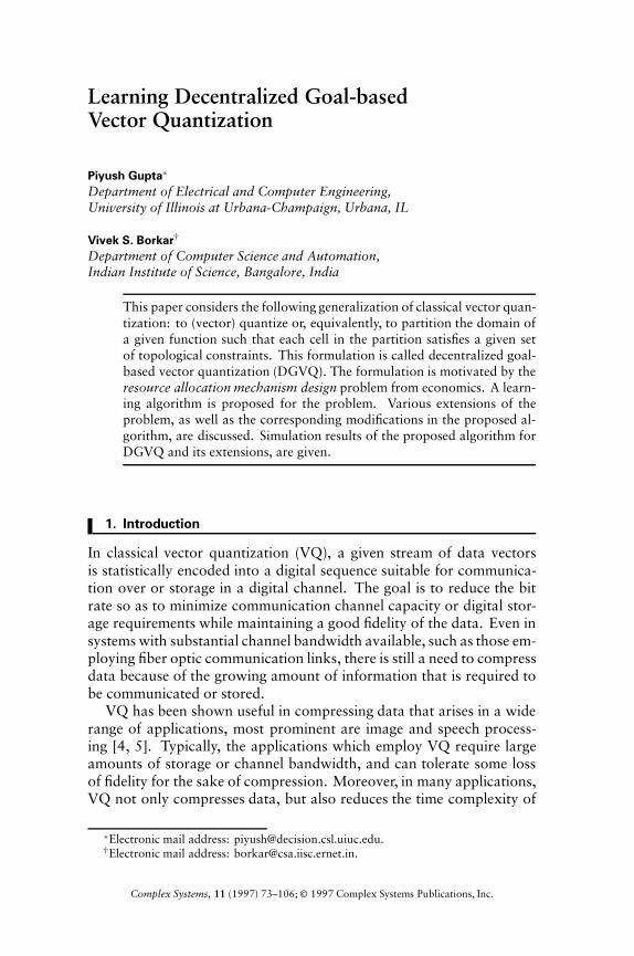
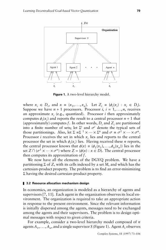
Figure 1. A two-level hierarchy model.

where xi Œ Di, and x # (x1, . . . , xn). Let Zi # {fi(xi) : xi Œ Di}.Suppose we have n + 1 processors. Processor i, i = 1, . . . , n, receivesan approximate xi (e.g., quantized). Processor i then approximatelycomputes fi(xi) and reports the result to a central processor n + 1 that(approximately) computes f . In other words, Di and Zi are partitionedinto a finite number of sets; let Si and si denote the typical sets ofthose partitionings. Also, let S #S 1 ¥µ ¥ Sn and s # s1 ¥µ ¥ sn.Processor i receives the set in which xi lies and reports to the centralprocessor the set in which fi(xi) lies. Having received these n reports,the central processor knows that f(x) # (f1(x1), . . . ,fn(xn)) lies in theset Z» (s1 ¥µ ¥ sn) where Z = {f(x) : x Œ D}. The central processorthen computes its approximation of f .

We now have all the elements of the DGVQ problem. We have apartitioning S of Z, with its cells indexed by a set M, and which has thecartesian-product property. The problem is to find an error-minimizingS having the desired cartesian-product property.

3.2 Resource allocation mechanism design

In economics, an organization is modeled as a hierarchy of agents andsupervisors [7, 11]. Each agent in the organization observes its local en-vironment. The organization is required to take an appropriate actionin response to the present environment. Since the relevant informationis initially dispersed among the agents, messages need to be exchangedamong the agents and their supervisors. The problem is to design opti-mal messages with respect to given criteria.

For example, consider a two-level hierarchy model composed of nagents A1, . . . , An, and a single supervisor S (Figure 1). Agent Ai observes



its local environment xi, which lies in a set Di. Let x # (x1, . . . , xn) andD # D1 ¥ D2 ¥ µ ¥ Dn. The organization would like to take anappropriate action, namely f (x) in response to the current environmentx; f (x) lies in some set A. f is referred to as the desired outcome function.Since information about x is initially dispersed among the n agents,we have to design a scheme in which some suitable communicationoccurs between the agents and the supervisor. In particular, we assumethat the organization will use a mechanism on D, which we have todesign. A mechanism on D is a triple p = [M, (m1, . . . ,mn), h], whereM # M1 ¥µ ¥ Mn is a set called the message space, with a typicalelement m, called a message; mi is a mapping from Di to Mi; and h,called the outcome function, is from M to A. One way to interpretthe operation of the mechanism is as follows: let qi be a quantizationmap on Di (i.e., qi maps Di to a finite subset Ci of Di), and let li bean indexing map on the image of qi (i.e., li maps Ci to {1, 2, . . . , |Ci|}).Agent Ai quantizes xi using qi and sends the index corresponding toqi(xi), li(qi(xi)), as message mi to the supervisor S (i.e., mi = li Î qi).Let m # (m1, . . . , mn), m Œ M, and l-1

i be the inverse map of li. ThenS outputs h(m) # f (l-1

1 (m1), . . . , l-1n (mn)) # f (q1(x1), . . . , qn(xn)) as the

response of the organization to the environment x. Now we wouldlike to find a mechanism p that minimizes the mean-square error Efrom equation (3.1) and is informationally least costly (i.e., with leastcommunication requirement between the agents and the supervisor).

The most widely studied measures of information costs are variousmeasures of the size of the message space M. In the bulk of the mech-anisms in the economics literature both the message space and the setof outcomes are either continua or discrete-but-infinite [11]. But realcommunication and computing technologies do not in fact permit amessage or an outcome to be a point of a continuum. Messages andoutcomes must be quantized, and the benefits of greater precision ofquantization have to be weighed against the costs (i.e., the number ofQ-levels). Accordingly, it is of considerable interest to study mecha-nisms in which message space and outcome set are not continua but are,rather, quantized as in the two-level hierarchy example above.

Hence we use bit complexity of the message space M as a measureof information cost. Moreover, instead of imposing hard constraints onthe bit size of the messages, we propose the following energy functionH:

H = ‡D

(¸ f (x) - f ( q1(x1), . . . , qn(xn) ) ¸2 )2 P(dx) + l $ S (3.2)

where l is a positive weighing factor and S is a bit-based complexitymeasure of the messages. Note that the choice of l will dictate thetradeoff between fidelity (i.e., lowering of distortion) and message com-plexity. Its choice perforce will involve some judgment, which makesit a “design parameter.” It will be interesting to come up with a theo-



retically justified choice, but no obvious choice offers itself. A similarcomment applies to equation (4.7) later.

In the two-level hierarchy example, S can be chosen as

S =n‚

i=1

log2 Ni

where Ni indicates the cardinality of the set qi(Di) (i.e., the number ofQ-levels for agent Ai).

4. An adaptive algorithm for decentralized goal-based vectorquantization

In this section we describe an adaptive algorithm for designing the quan-tization maps qi, i = 1, . . . , n, such that the energyH from equation (3.2)is minimized. The proposed algorithm is adaptive in the sense that ittries to improve its performance with every instance of the input-outputpair seen.

The basic idea is as follows. The algorithm starts by assigning afixed number of Q-levels, say 1, to each agent. It adapts qi, i = 1, . . . , n,using a Kohonen-like rule for a fixed number, say g, of input-outputpairs seen. Concurrently, it collects the error statistics for each agent.Based on the error statistics, the algorithm adds (deletes) a Q-level inqi* , where i* is the agent which induced maximum change in H in itsprevious adaptation. It again adapts qis for g input-output pairs. Thealgorithm repeats these two steps of adaptation and addition (deletion)of Q-levels until the energyH stops decreasing.

We now discuss in detail each of the steps involved in the algorithm.

4.1 Adaptation rule for single-agent case

Since we are interested in an adaptive algorithm, we seek a rule whichupdates the quantization maps qi after every input-output pair (x, f (x))seen, so as to minimize the energy functionH. In order to concentrate onthis step of the algorithm, we consider the following simplification of theproblem: Given m instances of the input-output pairs (x(k), f (x(k))), k =1, . . . , m, where {x(k)} are independent and identically drawn from Daccording to the probability distribution P. Also given is a fixed numberN. Consider a two-level hierarchy in which a single agent A reports tosupervisor S. The quantization map q of agent A has exactly N Q-levels.The problem is to adapt the map q, keeping the number of Q-levels fixedto N, so as to minimize the mean-square error E from equation (3.1).Note that the problem has the following constraints.

For a given pair (x, f (x)), x is known only to A and the desired out-come f (x) is known only to S. Hence gradient-based adaptation of thequantization map q cannot be done.



Since we consider bit-based complexity measure of the messages ex-changed between agent A and supervisor S (section 3.2), S can feedbackto A only discretized information about the error between the desiredoutcome f (x) and the response of the organization f (q (x)).

Probability distribution P is, in general, not known beforehand. Thus weuse the following empirical estimate of the error function instead:

E =1m

m‚k=1

(¸ f (x(k))- f ( q(x(k)) ) ¸2 )2. (4.1)

In section 2.1, we discussed the competitive learning (CL) algorithmfor VQ. We adapt the CL algorithm as our starting point and indicatehow it can be modified to tackle the present problem.

As observed before, supervisor S can only give to A discretized in-formation about the error between the desired outcome f (x) and theresponse of the organization f (q(x), ). In particular, let us consider thecase in which S can feedback to A only one bit of information about theerror. For this purpose, assume that the goal of adaptation is to reducethe mean-square error E below a prespecified e > 0, that is,

E # ‡D

(¸ f (x) - f (q(x)) ¸2 )2 P (dx) < e. (4.2)

Now we let S feedback to A the following reinforcement signal r:

r(k) = ; 1 if I¸ f (x(k)) - f ( q(x(k)) ) ¸2M2 < e,0 otherwise.

On receiving r, agent A adapts its Q-levels yi as follows:

yi(k + 1) = yi(k) + h(k) $ (x(k) - yi(k)) $ zi(k) $ (1 - r(k)) (4.3)

where h(k) is the learning rate, and zi(k) is as in equation (2.3). Inother words, agent A moves the winning Q-level towards the inputonly if the error exceeds a prespecified value. A particularly interestingchoice of h(k) is when it varies with different rates for different Q-levelsyi, i = 1, . . . , N, as follows:

hi(k) =1⁄k

j=1 zi(j) $ ( 1 - r(j) ) + 1(4.4)

which along with equation (4.3) gives

yi(k + 1) ª1⁄k

j=1 zi(j) $ ( 1 - r(j) ) + 1

$ÊÁÁÁÁÁÁË

k‚j=1

x(j) $ zi(j) $ ( 1 - r(j) ) + yi(0)ˆ˜˜¯

. (4.5)



That is, equation (4.3) adapts the quantization map q such that eachQ-level yi goes to the centroid of all x for which it is at the minimumdistance and representing x by yi causes the error to exceed e. Notethat yi(k + 1) is only approximately given by equation (4.5) because, inthe adaptation rule equation (4.3), yi is updated after every input x seenand, therefore, the region for which yi is at the minimum distance, ischanging.

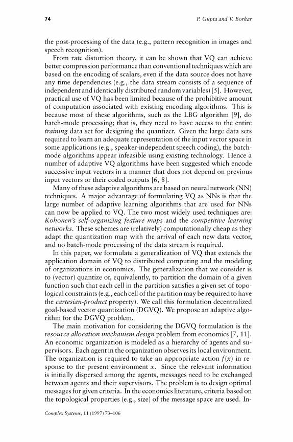
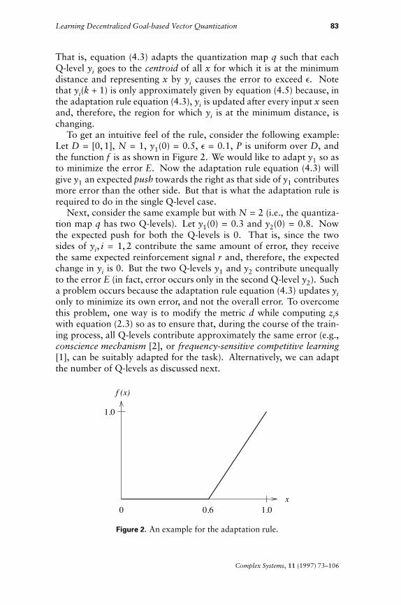
To get an intuitive feel of the rule, consider the following example:Let D = [0, 1], N = 1, y1(0) = 0.5, e = 0.1, P is uniform over D, andthe function f is as shown in Figure 2. We would like to adapt y1 so asto minimize the error E. Now the adaptation rule equation (4.3) willgive y1 an expected push towards the right as that side of y1 contributesmore error than the other side. But that is what the adaptation rule isrequired to do in the single Q-level case.

Next, consider the same example but with N = 2 (i.e., the quantiza-tion map q has two Q-levels). Let y1(0) = 0.3 and y2(0) = 0.8. Nowthe expected push for both the Q-levels is 0. That is, since the twosides of yi, i = 1, 2 contribute the same amount of error, they receivethe same expected reinforcement signal r and, therefore, the expectedchange in yi is 0. But the two Q-levels y1 and y2 contribute unequallyto the error E (in fact, error occurs only in the second Q-level y2). Sucha problem occurs because the adaptation rule equation (4.3) updates yionly to minimize its own error, and not the overall error. To overcomethis problem, one way is to modify the metric d while computing ziswith equation (2.3) so as to ensure that, during the course of the train-ing process, all Q-levels contribute approximately the same error (e.g.,conscience mechanism [2], or frequency-sensitive competitive learning[1], can be suitably adapted for the task). Alternatively, we can adaptthe number of Q-levels as discussed next.

x

f (x)

0.6 1.00

1.0

Figure 2. An example for the adaptation rule.



4.1.1 Adaptation of the number of quantization levels

This step of the algorithm helps not only in overcoming the limitationsof the adaptation rule, but also in avoiding the requirement of a prespec-ified number of Q-levels. Moreover, this step becomes essential whenthere is more than one agent in the problem. But let us first consider thesingle-agent case.

We start by assigning two Q-levels to A (i.e., N = 2). We nextadapt these Q-levels using the adaptation rule equation (4.3) for a fixednumber, say g, of input-output pairs. Also, we collect the error statisticsfor each Q-level; that is, we keep count of the number of times the ithQ-level has received the reinforcement signal r as 0, denoted by Ei. Thenthe value of Ei, after k input-output pairs have been seen, is

Ei(k) =k‚

j=1

zi(j) $ ( 1 - r(j) )

where zi is as in equation (4.3).After the completion of g adaptation steps, consider an estimate of

the mean-square error E = ⁄Ni=1 Ei. If E < e, then we are done as the aim

of equation (4.2) has been achieved. Otherwise, we add a Q-level yN+1between the maximum-error Q-level and its maximum-error neighbor.Specifically, let i* = arg max1£i£N Ei. Then add a Q-level between Q-level i* and its maximum-error neighbor. Two Q-levels are said to beneighbors if their regions have a common boundary, that is, let si be theregion associated with ith Q-level, yi (i.e., si = {x : arg minj ¸ x - yj ¸2=i}), then yi and yj are neighbors if si » sj " !, where si refers to theclosure of the set si). Let NE(i) be the set of all Q-levels which areneighbors of i, and let b(i) = arg maxkŒNE(i*) Ek. Then a Q-level is addedbetween the maximum-error Q-level i* and its maximum-error neighborb(i*). The newly added Q-level yN+1 is initialized as:

yN+1 =yi* $ Ei* + yj $ Eb(i*)

Ei* + Eb(i*).

This procedure requires knowledge of the neighborhood set of eachQ-level. A number of techniques exist to iteratively compute the neigh-borhood sets ([3, 12], and references therein). However, all of themare computation-intensive and impose specific restrictions on the topol-ogy of the Q-levels. We, therefore, use a crude-but-simple procedure:split the maximum-error Q-level i* into two Q-levels i*new and (N + 1).Let j = arg maxk"i* Ek, that is, j is the maximum-error-but-one Q-level.Then the new Q-levels are computed as

yi*new= yi* + D $ (yj - yi*), and

yN+1 = yi* - D $ (yj - yi*) (4.6)



(a) (b)

i

j

*

j

N+1i *new

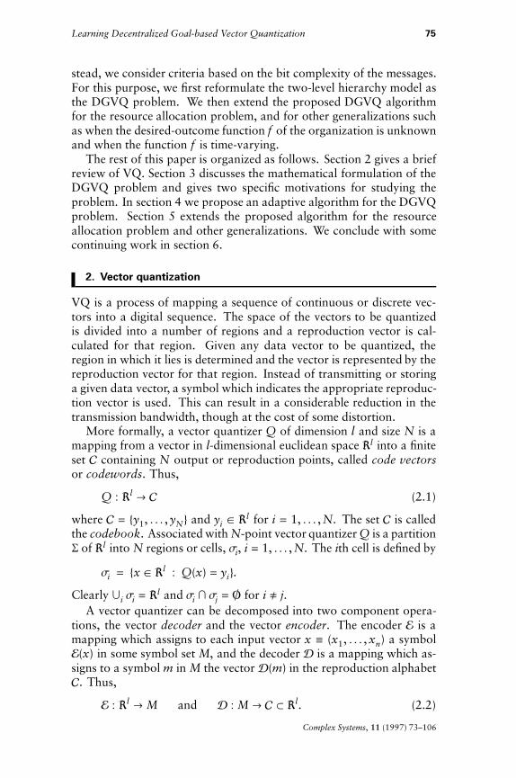
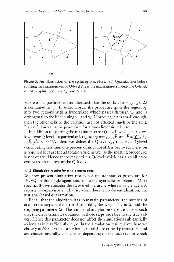
Figure 3. An illustration of the splitting procedure. (a) Quantization beforesplitting the maximum-error Q-level i*, j is the maximum-error-but-one Q-level.(b) After splitting i* into i*new and N + 1.

where D is a positive real number such that the set {x : ¸ x - yi* ¸2 £ D}is contained in si*. In other words, the procedure splits the region si*

into two regions with a hyperplane which passes through yi* and isorthogonal to the line joining yi* and yj. Moreover, if D is small enough,then the other cells of the partition are not affected much by the split.Figure 3 illustrates the procedure for a two-dimensional case.

In addition to splitting the maximum-error Q-level, we delete a very-low-error Q-level. In particular, let im = arg min1£i£N Ei and E = ⁄N

i=1 Ei.If Eim

/E < 0.1/N, then we delete the Q-level im, that is, a Q-levelcontributing less than one percent of its share of E is removed. Deletionis required because the adaptation rule, as well as the splitting procedure,is not exact. Hence there may exist a Q-level which has a small errorcompared to the rest of the Q-levels.

4.1.2 Simulation results for single-agent case

We now present simulation results for the adaptation procedure forDGVQ in the single-agent case on some synthetic problems. Morespecifically, we consider the two-level hierarchy where a single agent Areports to supervisor S. That is, when there is no decentralization, butjust goal-based quantization.

Recall that the algorithm has four main parameters: the number ofadaptation steps g, the error threshold e, the weight factor l, and thestopping parameterDe. The number of adaptation steps g is chosen suchthat the error estimates obtained in those steps are close to the true val-ues. Hence this parameter does not affect the simulations substantiallyas long as it is sufficiently large. In the simulation results given here wechose g = 200. On the other hand, e and l are critical parameters, andare chosen carefully. e is chosen depending on the accuracy to which



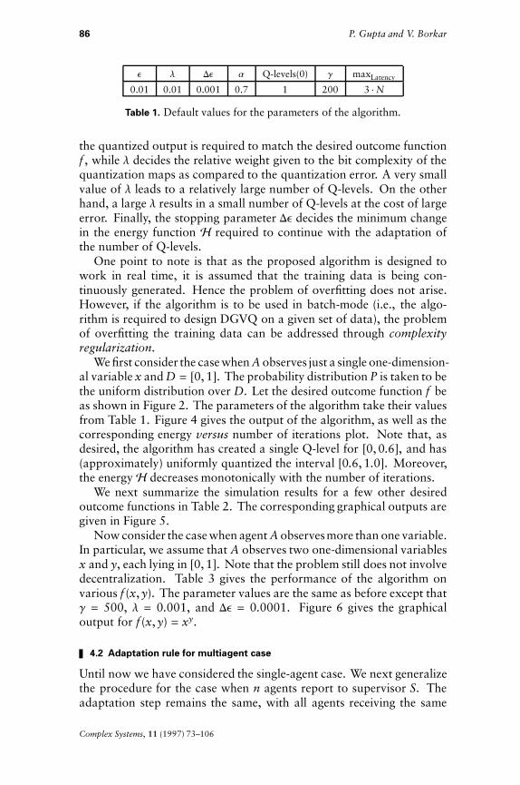
e l De a Q-levels(0) g maxLatency

0.01 0.01 0.001 0.7 1 200 3 $N

Table 1. Default values for the parameters of the algorithm.

the quantized output is required to match the desired outcome functionf , while l decides the relative weight given to the bit complexity of thequantization maps as compared to the quantization error. A very smallvalue of l leads to a relatively large number of Q-levels. On the otherhand, a large l results in a small number of Q-levels at the cost of largeerror. Finally, the stopping parameter De decides the minimum changein the energy function H required to continue with the adaptation ofthe number of Q-levels.

One point to note is that as the proposed algorithm is designed towork in real time, it is assumed that the training data is being con-tinuously generated. Hence the problem of overfitting does not arise.However, if the algorithm is to be used in batch-mode (i.e., the algo-rithm is required to design DGVQ on a given set of data), the problemof overfitting the training data can be addressed through complexityregularization.

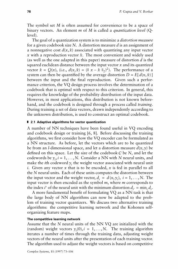
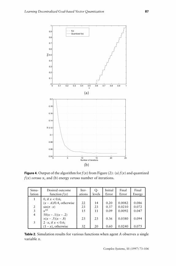
We first consider the case when A observes just a single one-dimension-al variable x and D = [0, 1]. The probability distribution P is taken to bethe uniform distribution over D. Let the desired outcome function f beas shown in Figure 2. The parameters of the algorithm take their valuesfrom Table 1. Figure 4 gives the output of the algorithm, as well as thecorresponding energy versus number of iterations plot. Note that, asdesired, the algorithm has created a single Q-level for [0, 0.6], and has(approximately) uniformly quantized the interval [0.6, 1.0]. Moreover,the energyH decreases monotonically with the number of iterations.

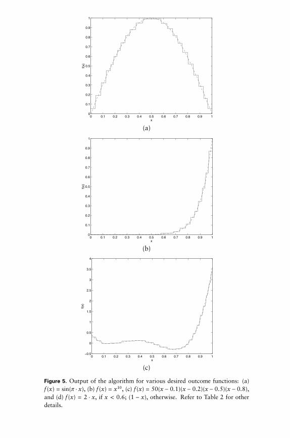
We next summarize the simulation results for a few other desiredoutcome functions in Table 2. The corresponding graphical outputs aregiven in Figure 5.

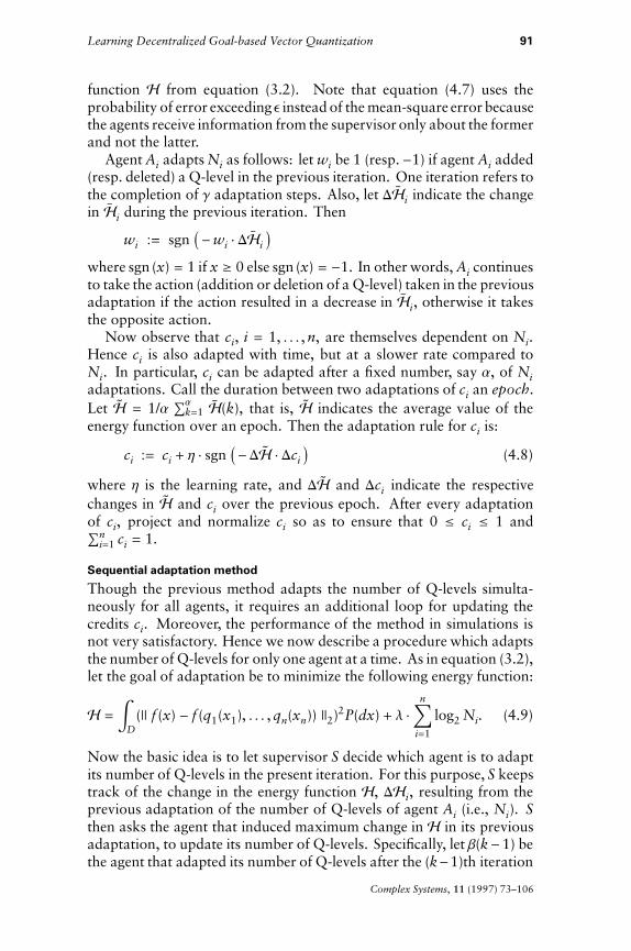
Now consider the case when agent A observesmore than one variable.In particular, we assume that A observes two one-dimensional variablesx and y, each lying in [0, 1]. Note that the problem still does not involvedecentralization. Table 3 gives the performance of the algorithm onvarious f (x, y). The parameter values are the same as before except thatg = 500, l = 0.001, and De = 0.0001. Figure 6 gives the graphicaloutput for f (x, y) = xy.

4.2 Adaptation rule for multiagent case

Until now we have considered the single-agent case. We next generalizethe procedure for the case when n agents report to supervisor S. Theadaptation step remains the same, with all agents receiving the same



f(x) Quantized f(x)

0 0.1 0.2 0.3 0.4 0.5 0.6 0.7 0.8 0.9 10

0.1

0.2

0.3

0.4

0.5

0.6

0.7

0.8

0.9

1

x

f(x)

(a)

0 5 10 15 20 250.04

0.06

0.08

0.1

0.12

0.14

0.16

0.18

0.2

Number of iterations

H

(b)

Figure 4. Output of the algorithm for f (x) from Figure (2): (a) f (x) and quantizedf (x) versus x, and (b) energy versus number of iterations.

Simu- Desired outcome Iter- Q- Initial Final Finallation function f (x) ations levels Error Error Energy

1 0, if x < 0.6;(x - .6)/0.4, otherwise 22 14 0.20 0.0082 0.086

2 sin(p $ x) 23 23 0.37 0.0210 0.0723 x10 15 11 0.09 0.0092 0.0474 50(x - .1)(x - .2)

¥(x - .5)(x - .8) 23 23 0.36 0.0380 0.0945 2 $ x, if x < 0.6;

(1 - x), otherwise 32 20 0.60 0.0240 0.075

Table 2. Simulation results for various functions when agent A observes a singlevariable x.


0 0.1 0.2 0.3 0.4 0.5 0.6 0.7 0.8 0.9 10

0.1

0.2

0.3

0.4

0.5

0.6

0.7

0.8

0.9

1

x

f(x)

(a)

0 0.1 0.2 0.3 0.4 0.5 0.6 0.7 0.8 0.9 10

0.1

0.2

0.3

0.4

0.5

0.6

0.7

0.8

0.9

1

x

f(x)

(b)

0 0.1 0.2 0.3 0.4 0.5 0.6 0.7 0.8 0.9 1−0.5

0

0.5

1

1.5

2

2.5

3

3.5

4

x

f(x)

(c)

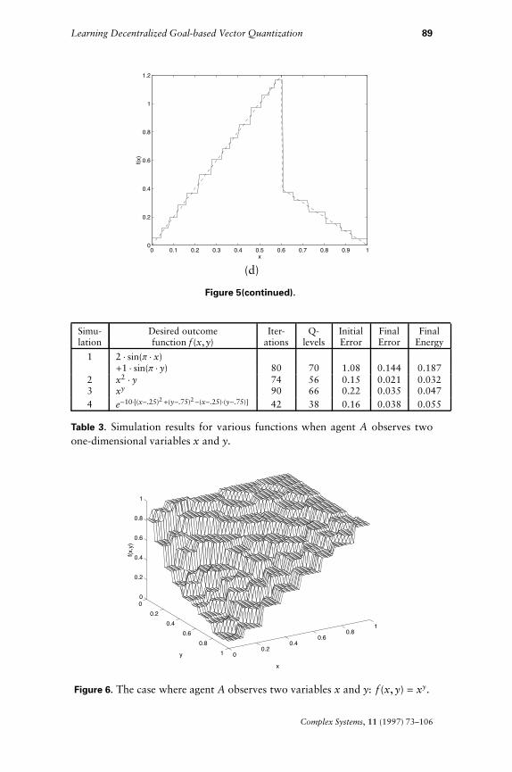
Figure 5. Output of the algorithm for various desired outcome functions: (a)f (x) = sin(p $ x), (b) f (x) = x10, (c) f (x) = 50(x- 0.1)(x- 0.2)(x- 0.5)(x - 0.8),and (d) f (x) = 2 $ x, if x < 0.6; (1 - x), otherwise. Refer to Table 2 for otherdetails.


0 0.1 0.2 0.3 0.4 0.5 0.6 0.7 0.8 0.9 10

0.2

0.4

0.6

0.8

1

1.2

x

f(x)

(d)

Figure 5(continued).

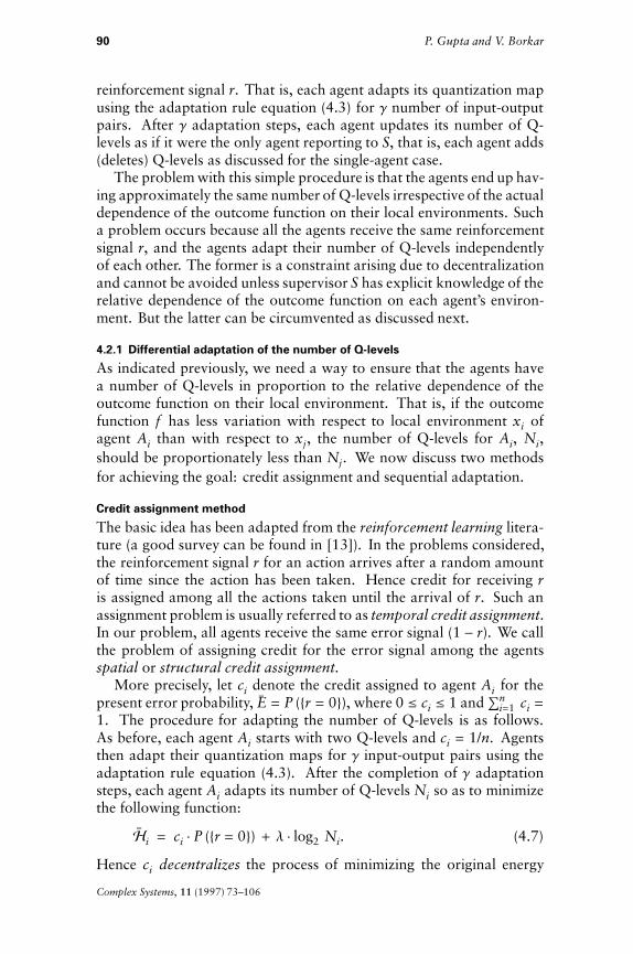
Simu- Desired outcome Iter- Q- Initial Final Finallation function f (x,y) ations levels Error Error Energy

1 2 $ sin(p $ x)+1 $ sin(p $ y) 80 70 1.08 0.144 0.187

2 x2 $ y 74 56 0.15 0.021 0.0323 xy 90 66 0.22 0.035 0.0474 e-10$[(x-.25)2 +(y-.75)2-(x-.25)$(y-.75)] 42 38 0.16 0.038 0.055

Table 3. Simulation results for various functions when agent A observes twoone-dimensional variables x and y.

00.2

0.40.6

0.81

00.2

0.40.6

0.81

0

0.2

0.4

0.6

0.8

1

x

y

f(x,y

)

Figure 6. The case where agent A observes two variables x and y: f (x, y) = xy.



reinforcement signal r. That is, each agent adapts its quantization mapusing the adaptation rule equation (4.3) for g number of input-outputpairs. After g adaptation steps, each agent updates its number of Q-levels as if it were the only agent reporting to S, that is, each agent adds(deletes) Q-levels as discussed for the single-agent case.

The problem with this simple procedure is that the agents end up hav-ing approximately the same number of Q-levels irrespective of the actualdependence of the outcome function on their local environments. Sucha problem occurs because all the agents receive the same reinforcementsignal r, and the agents adapt their number of Q-levels independentlyof each other. The former is a constraint arising due to decentralizationand cannot be avoided unless supervisor S has explicit knowledge of therelative dependence of the outcome function on each agent’s environ-ment. But the latter can be circumvented as discussed next.

4.2.1 Differential adaptation of the number of Q-levels

As indicated previously, we need a way to ensure that the agents havea number of Q-levels in proportion to the relative dependence of theoutcome function on their local environment. That is, if the outcomefunction f has less variation with respect to local environment xi ofagent Ai than with respect to xj, the number of Q-levels for Ai, Ni,should be proportionately less than Nj. We now discuss two methodsfor achieving the goal: credit assignment and sequential adaptation.

Credit assignment method

The basic idea has been adapted from the reinforcement learning litera-ture (a good survey can be found in [13]). In the problems considered,the reinforcement signal r for an action arrives after a random amountof time since the action has been taken. Hence credit for receiving ris assigned among all the actions taken until the arrival of r. Such anassignment problem is usually referred to as temporal credit assignment.In our problem, all agents receive the same error signal (1 - r). We callthe problem of assigning credit for the error signal among the agentsspatial or structural credit assignment.

More precisely, let ci denote the credit assigned to agent Ai for thepresent error probability, E = P ({r = 0}), where 0 £ ci £ 1 and⁄n

i=1 ci =1. The procedure for adapting the number of Q-levels is as follows.As before, each agent Ai starts with two Q-levels and ci = 1/n. Agentsthen adapt their quantization maps for g input-output pairs using theadaptation rule equation (4.3). After the completion of g adaptationsteps, each agent Ai adapts its number of Q-levels Ni so as to minimizethe following function:

Hi = ci $ P ({r = 0}) + l $ log2 Ni. (4.7)

Hence ci decentralizes the process of minimizing the original energy



function H from equation (3.2). Note that equation (4.7) uses theprobability of error exceeding e instead of the mean-square error becausethe agents receive information from the supervisor only about the formerand not the latter.

Agent Ai adapts Ni as follows: let wi be 1 (resp.-1) if agent Ai added(resp. deleted) a Q-level in the previous iteration. One iteration refers tothe completion of g adaptation steps. Also, let DHi indicate the changein Hi during the previous iteration. Then

wi := sgn I-wi $ DHi Mwhere sgn (x) = 1 if x % 0 else sgn (x) = -1. In other words, Ai continuesto take the action (addition or deletion of a Q-level) taken in the previousadaptation if the action resulted in a decrease in Hi, otherwise it takesthe opposite action.

Now observe that ci, i = 1, . . . , n, are themselves dependent on Ni.Hence ci is also adapted with time, but at a slower rate compared toNi. In particular, ci can be adapted after a fixed number, say a, of Niadaptations. Call the duration between two adaptations of ci an epoch.Let H = 1/a ⁄ak=1 H(k), that is, H indicates the average value of theenergy function over an epoch. Then the adaptation rule for ci is:

ci := ci + h $ sgn I-DH $ Dci M (4.8)

where h is the learning rate, and DH and Dci indicate the respectivechanges in H and ci over the previous epoch. After every adaptationof ci, project and normalize ci so as to ensure that 0 £ ci £ 1 and⁄n

i=1 ci = 1.

Sequential adaptation method

Though the previous method adapts the number of Q-levels simulta-neously for all agents, it requires an additional loop for updating thecredits ci. Moreover, the performance of the method in simulations isnot very satisfactory. Hence we now describe a procedure which adaptsthe number of Q-levels for only one agent at a time. As in equation (3.2),let the goal of adaptation be to minimize the following energy function:

H = ‡D

(¸ f (x) - f (q1(x1), . . . , qn(xn)) ¸2)2P(dx) + l $n‚

i=1

log2 Ni. (4.9)

Now the basic idea is to let supervisor S decide which agent is to adaptits number of Q-levels in the present iteration. For this purpose, S keepstrack of the change in the energy function H, DHi, resulting from theprevious adaptation of the number of Q-levels of agent Ai (i.e., Ni). Sthen asks the agent that induced maximum change in H in its previousadaptation, to update its number of Q-levels. Specifically, let b(k-1) bethe agent that adapted its number of Q-levels after the (k-1)th iteration



(recall that one iteration refers to the completion of g adaptation steps).Also, let

wi(k - 1) =

ÏÔÔÔÔÔÔÔÌÔÔÔÔÔÔÔÓ

+1 if i = b(k - 1) andb(k - 1) added a Q-level,

-1 if i = b(k - 1) andb(k - 1) deleted a Q-level,

wi(k - 2) otherwise.

That is, wi = 1 (resp. -1) indicates that agent Ai added (resp. deleted) aQ-level in its previous adaptation of the number of Q-levels. Next, let

DHi(k) = ; H(k) -H(k - 1) if i = b(k - 1),DHi(k - 1) otherwise. (4.10)

Then, after the kth iteration, S asks the b(k)th agent to update its numberof Q-levels according to wb(k)(k), where

b(k) = arg max1£i£N

| DHi(k) |

wb(k)(k) = sgn (-wb(k)(k - 1) $ DHb(k)(k) ). (4.11)

Equivalently, S asks the b(k)th agent to add a Q-level if either its previousadaptation was the addition of a Q-level that resulted in a reduction ofH, or its previous adaptation was the deletion of a Q-level that increasedH. Otherwise, S asks b(k) to delete a Q-level.

This procedure is repeated until maxi |DHi(k)| < De, where De > 0is a prespecified value. In other words, the training process is stopped ifnone of the agents are able to substantially reduce the energy functionby adapting its number of Q-levels.

For this procedure we assumed that we had an exact estimate ofH(k),an optimal adaptation rule, and an optimal splitting procedure. Sincethat is not the case, we further modify the procedure as follows.

SinceH(k) is estimated from a finite number of samples, it will have somevariance around a mean value. To reduce the effect of this variance, weaverage DHi(k) as follows:

DHi(k) = ; a $ DHi(k - 1) + (1 - a) $ IH(k) -H(k - 1)M if i = b(k - 1),DHi(k - 1) otherwise

where a Œ [0, 1].

In general, DHi is dependent not only on Ni, but also on the number ofQ-levels in the quantization maps of the rest of the agents. For example,consider the case where two agents, each observing one variable x and y,report to supervisor S. Let the desired outcome function be f (x, y) = xy.Then the change in the energy function due to adaptation of the numberof Q-levels of x is also dependent on the current number of Q-levels for



y. Now, in one iteration, only one agent updates its DHi. Hence it ispossible that an agent last adapted its number of Q-levels (and thus itsDHi) a large number of iterations ago. In such a case, that agent’s DHimay not be a true reflection of the agent’s potential in reducing the energyfunction.

Therefore, if an agent, say i0, has not updated its DHi0for the last

maxLatency number of iterations, then b(k) is set to i0 and wi0(k) = 1 (i.e,

i0 adds a Q-level, so as to update its DHi0). maxLatency is taken to be a

multiple of the number of agents in the organization.

Finally, since the adaptation rule, as well as the splitting procedure, isnonoptimal, each agent periodically deletes a very-low-error Q-level. Thisdeletion is separate from the deletion due to equation (4.11).

Remark 4.1. In this algorithm, we have assumed that supervisor S canfeedback to agents only a single bit of information about the quantiza-tion error E; that is, the reinforcement signal r can take only two values,0 or 1. The algorithm can be easily extended to the more general case:when S can feedback l bits of information. The supervisornow transmitsto agents an l-bit reinforcement signal, r # (rl, . . . , r1) Œ {0, 1}l, whichencodes the quantization error E such that a higher value of r indicateslower E. Let R : {0, 1}l Æ [0, 1], be defined by R(r) = 1/2l⁄l

i=1 2i-1 $ ri.Then the agents adapt their quantization maps using the adaptation ruleequation (4.3), with r being replaced by R(r). The rest of the algorithmremains the same.

Remark 4.2. While arriving at this algorithm, we have assumed thatsupervisor S has knowledge of the quantization map qi of agent Ai,for each i. But Ai adapts qi after every input-output pair seen by theorganization, and therefore, Ai needs to transmit the changes in qi toS. For this purpose we can discretize the adaptation rule, that is, qi isallowed to take values only over a prespecified grid on Di. Then, afterevery adaptation of qi, Ai transmits the number of steps by which qihas moved over the grid. Or, to reduce the communication overhead,Ai can transmit to S the net change in its quantization map qi afterthe completion of each iteration (i.e., g adaptation steps), and not afterevery adaptation step.

4.2.2 Simulation results for multiagent case

We now present simulation results for the given procedure for DGVQin the multiagent case. We first discuss the case when two agents, A1and A2, report to supervisor S. Moreover, for the sake of simplicity,we assume that A1 and A2 observe only one variable each: x and yrespectively.

We first consider the desired outcome function f (x, y) to be such thatdecentralization of the quantization process is “natural,” that is, f (x, y)



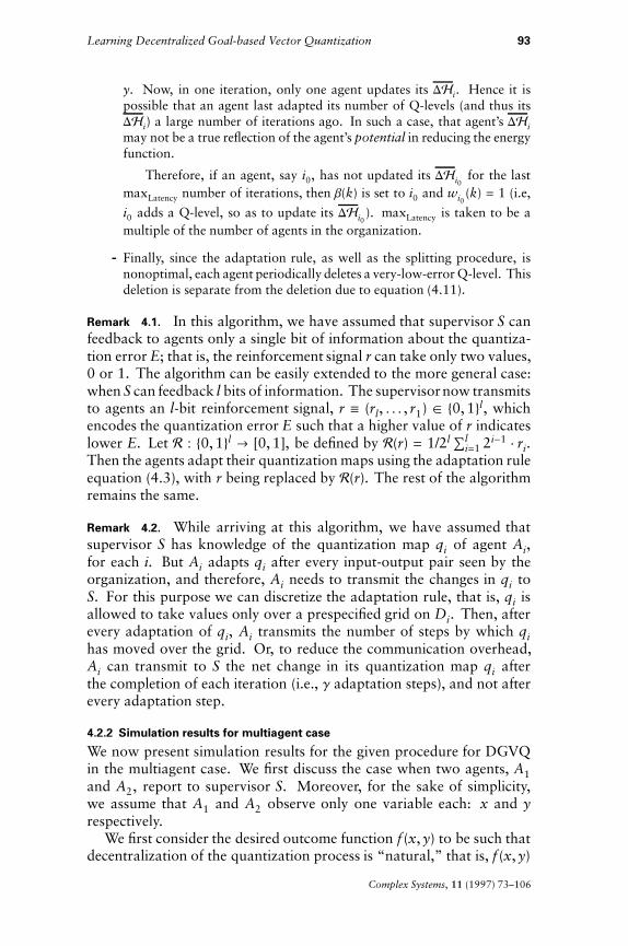
Simu- A B Iter- Q-levels Q-levels Initial Final Finallation ations for x for y Error Error Energy

1 2.0 2.0 50 23 22 1.45 0.063 0.352 1.0 2.0 40 14 23 1.10 0.056 0.323 0.5 2.0 40 8 23 0.92 0.056 0.304 0.0 2.0 36 1 20 0.74 0.050 0.205 2.0 0.0 33 23 1 0.71 0.042 0.216 2.0 0.5 35 20 8 0.90 0.060 0.307 2.0 1.0 39 22 14 1.08 0.059 0.32

Table 4. Simulation results for the two-agent case. The agents observe onevariable each, x and y respectively. The desired outcome function is f (x, y) =A $ sin(p $ x) + B $ sin(p $ y).

Simu- Desired outcome Iter- Q Q Initial Final Finallation function f (x, y) ations for x for y Error Error Energy

1 x2 $ y 37 16 14 0.15 0.011 0.0922 xy 34 17 12 0.22 0.018 0.0993 e-10[(x-.25)2+(y-.75)2-(x-.25)(y-.75)] 42 14 19 0.16 0.015 0.0594 4 sin(p $ x $ y) 41 17 21 1.29 0.088 0.370

Table 5. Simulation results for various f (x, y) for the two-agent case.

can be written as g(x) + h(y). In particular, we consider

f (x, y) = A $ sin(p $ x) + B $ sin(p $ y) (4.12)

where A, B Œ ¬. Table 4 gives the outputs of the algorithm for variousvalues of A and B. The parameter values are taken from Table 1.Note that, as the result of using differential adaptation of Q-levels(section 4.2.1), the algorithm creates the number of Q-levels for the twoagents in proportion to the relative dependence of the outcome functionon their local environments.

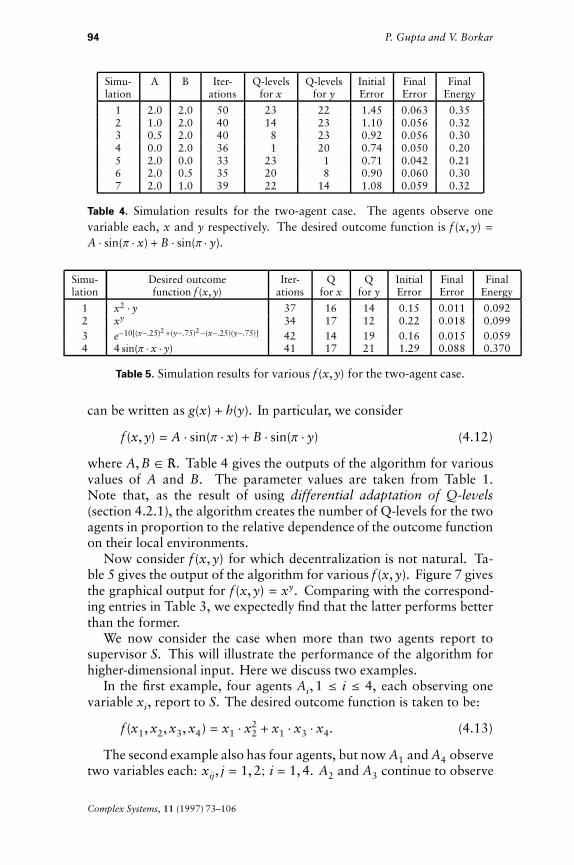
Now consider f (x, y) for which decentralization is not natural. Ta-ble 5 gives the output of the algorithm for various f (x, y). Figure 7 givesthe graphical output for f (x, y) = xy. Comparing with the correspond-ing entries in Table 3, we expectedly find that the latter performs betterthan the former.

We now consider the case when more than two agents report tosupervisor S. This will illustrate the performance of the algorithm forhigher-dimensional input. Here we discuss two examples.

In the first example, four agents Ai, 1 £ i £ 4, each observing onevariable xi, report to S. The desired outcome function is taken to be:

f (x1, x2, x3, x4) = x1 $ x22 + x1 $ x3 $ x4. (4.13)

The second example also has four agents, but now A1 and A4 observetwo variables each: xij, j = 1, 2; i = 1, 4. A2 and A3 continue to observe



00.2

0.40.6

0.81

00.2

0.40.6

0.81

0

0.2

0.4

0.6

0.8

1

x

y

f(x,y

)

Figure 7. Two-agent case, each agent observes one variable (x and y resp.),f (x, y) = xy.

Simu- f ($) Iter- Q Q Q Q Initial Final Finallation ations for A1 for A2 for A3 for A4 Error Error Energy

1 (4.13) 88 27 22 17 13 0.21 0.014 0.0322 (4.14) 285 46 35 25 79 0.64 0.120 0.340

Table 6. Two examples for the four-agent case.

one variable each. The desired outcome function is:

f (x) = x11 $ sin(p $ x2) + 2 $ x12 $ x23 $ x41 + e-5(x42-0.25)(x3-0.6). (4.14)

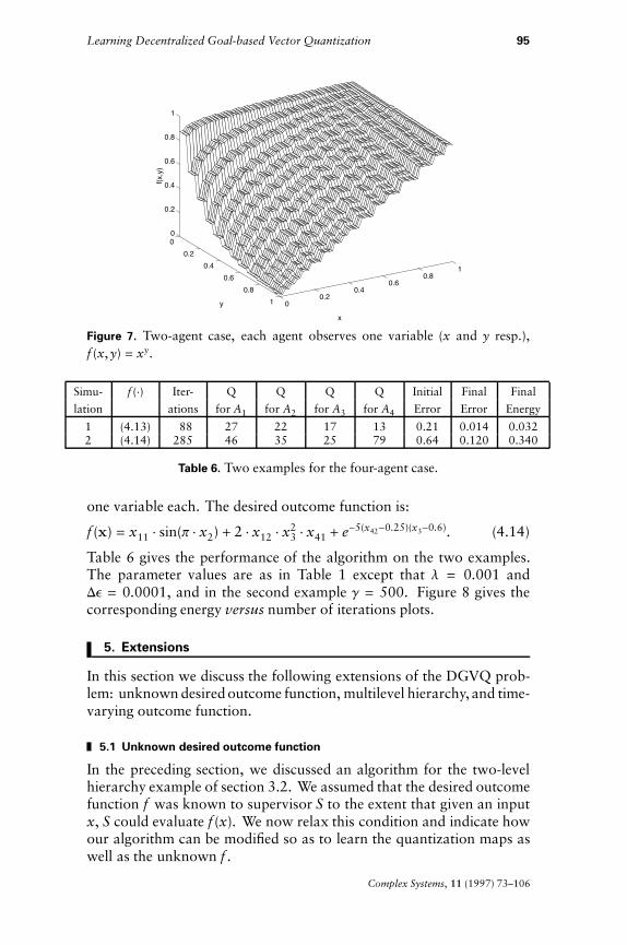
Table 6 gives the performance of the algorithm on the two examples.The parameter values are as in Table 1 except that l = 0.001 andDe = 0.0001, and in the second example g = 500. Figure 8 gives thecorresponding energy versus number of iterations plots.

5. Extensions

In this section we discuss the following extensions of the DGVQ prob-lem: unknown desired outcome function, multilevel hierarchy, and time-varying outcome function.

5.1 Unknown desired outcome function

In the preceding section, we discussed an algorithm for the two-levelhierarchy example of section 3.2. We assumed that the desired outcomefunction f was known to supervisor S to the extent that given an inputx, S could evaluate f (x). We now relax this condition and indicate howour algorithm can be modified so as to learn the quantization maps aswell as the unknown f .



0 10 20 30 40 50 60 70 80 900.02

0.04

0.06

0.08

0.1

0.12

0.14

0.16

0.18

0.2

0.22


H

(a)

0 50 100 150 200 250 3000.3

0.4

0.5

0.6

0.7

0.8

0.9


H

(b)

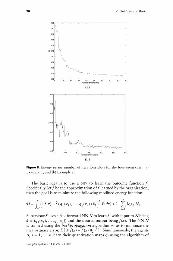
Figure 8. Energy versus number of iterations plots for the four-agent case: (a)Example 1, and (b) Example 2.

The basic idea is to use a NN to learn the outcome function f .Specifically, let f be the approximation of f learned by the organization,then the goal is to minimize the following modified energy function:

H = ‡DJ¸ f (x) - f ( q1(x1), . . . , qn(xn) ) ¸2 N2 P(dx) + l $

n‚i=1

log2 Ni.

Supervisor S uses a feedforward NNN to learn f , with input to N beingx # (q1(x1), . . . , qn(xn)) and the desired output being f (x). The NN Nis trained using the backpropagation algorithm so as to minimize themean-square error, E [ (¸ f (x) - f (x) ¸2 )2 ]. Simultaneously, the agentsAi, i = 1, . . . , n learn their quantization maps qi using the algorithm of



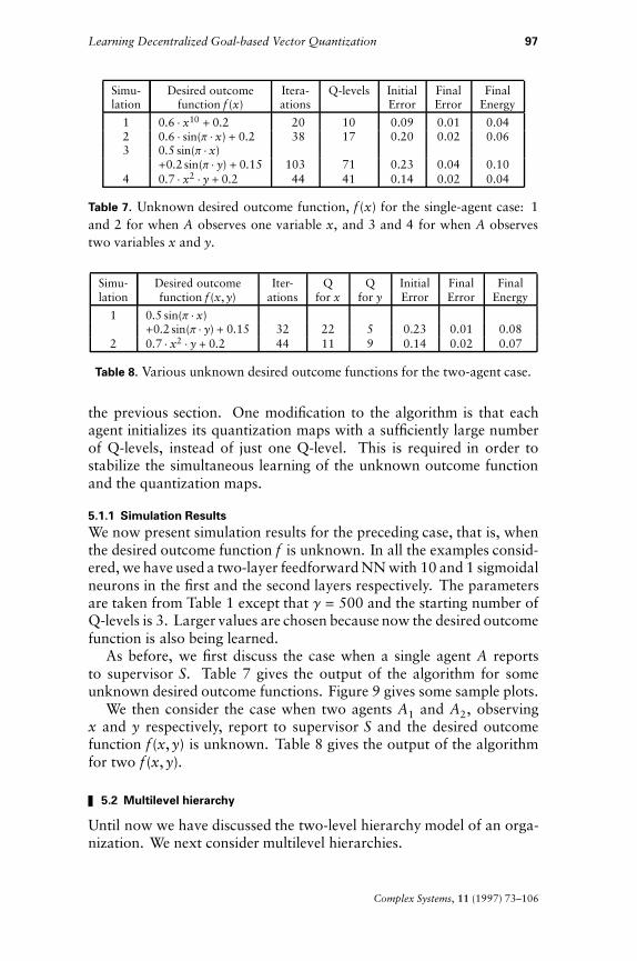
Simu- Desired outcome Itera- Q-levels Initial Final Finallation function f (x) ations Error Error Energy

1 0.6 $ x10 + 0.2 20 10 0.09 0.01 0.042 0.6 $ sin(p $ x) + 0.2 38 17 0.20 0.02 0.063 0.5 sin(p $ x)

+0.2 sin(p $ y) + 0.15 103 71 0.23 0.04 0.104 0.7 $ x2 $ y + 0.2 44 41 0.14 0.02 0.04

Table 7. Unknown desired outcome function, f (x) for the single-agent case: 1and 2 for when A observes one variable x, and 3 and 4 for when A observestwo variables x and y.

Simu- Desired outcome Iter- Q Q Initial Final Finallation function f (x, y) ations for x for y Error Error Energy

1 0.5 sin(p $ x)+0.2 sin(p $ y) + 0.15 32 22 5 0.23 0.01 0.08

2 0.7 $ x2 $ y + 0.2 44 11 9 0.14 0.02 0.07

Table 8. Various unknown desired outcome functions for the two-agent case.

the previous section. One modification to the algorithm is that eachagent initializes its quantization maps with a sufficiently large numberof Q-levels, instead of just one Q-level. This is required in order tostabilize the simultaneous learning of the unknown outcome functionand the quantization maps.

5.1.1 Simulation ResultsWe now present simulation results for the preceding case, that is, whenthe desired outcome function f is unknown. In all the examples consid-ered, we have used a two-layer feedforward NN with 10 and 1 sigmoidalneurons in the first and the second layers respectively. The parametersare taken from Table 1 except that g = 500 and the starting number ofQ-levels is 3. Larger values are chosen because now the desired outcomefunction is also being learned.

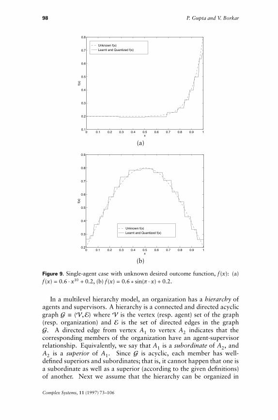
As before, we first discuss the case when a single agent A reportsto supervisor S. Table 7 gives the output of the algorithm for someunknown desired outcome functions. Figure 9 gives some sample plots.

We then consider the case when two agents A1 and A2, observingx and y respectively, report to supervisor S and the desired outcomefunction f (x, y) is unknown. Table 8 gives the output of the algorithmfor two f (x, y).

5.2 Multilevel hierarchy

Until now we have discussed the two-level hierarchy model of an orga-nization. We next consider multilevel hierarchies.



Unknown f(x) Learnt and Quantized f(x)

0 0.1 0.2 0.3 0.4 0.5 0.6 0.7 0.8 0.9 10.1

0.2

0.3

0.4

0.5

0.6

0.7

0.8

x

f(x)

(a)

Unknown f(x) Learnt and Quantized f(x)

0 0.1 0.2 0.3 0.4 0.5 0.6 0.7 0.8 0.9 10.2

0.3

0.4

0.5

0.6

0.7

0.8

0.9

x

f(x)

(b)

Figure 9. Single-agent case with unknown desired outcome function, f (x): (a)f (x) = 0.6 $ x10 + 0.2, (b) f (x) = 0.6 * sin(p $ x) + 0.2.

In a multilevel hierarchy model, an organization has a hierarchy ofagents and supervisors. A hierarchy is a connected and directed acyclicgraph G # (V,E) where V is the vertex (resp. agent) set of the graph(resp. organization) and E is the set of directed edges in the graphG. A directed edge from vertex A1 to vertex A2 indicates that thecorresponding members of the organization have an agent-supervisorrelationship. Equivalently, we say that A1 is a subordinate of A2, andA2 is a superior of A1. Since G is acyclic, each member has well-defined superiors and subordinates; that is, it cannot happen that one isa subordinate as well as a superior (according to the given definitions)of another. Next we assume that the hierarchy can be organized in



x31 x32 x33

A32

A22

A11

A31

A21

x21

11x

x22

33A

f(x)

Figure 10. A three-level hierarchy model. Aij is the jth agent in the ith level ofthe hierarchy.

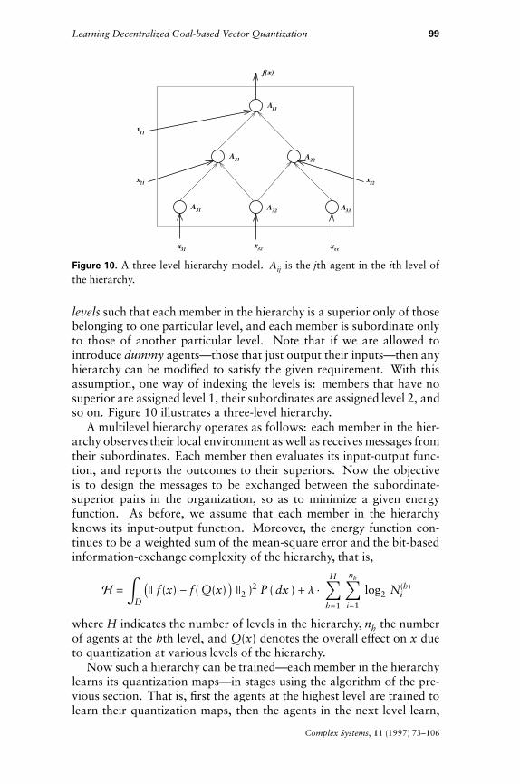
levels such that each member in the hierarchy is a superior only of thosebelonging to one particular level, and each member is subordinate onlyto those of another particular level. Note that if we are allowed tointroduce dummy agents—those that just output their inputs—then anyhierarchy can be modified to satisfy the given requirement. With thisassumption, one way of indexing the levels is: members that have nosuperior are assigned level 1, their subordinates are assigned level 2, andso on. Figure 10 illustrates a three-level hierarchy.

A multilevel hierarchy operates as follows: each member in the hier-archy observes their local environment as well as receives messages fromtheir subordinates. Each member then evaluates its input-output func-tion, and reports the outcomes to their superiors. Now the objectiveis to design the messages to be exchanged between the subordinate-superior pairs in the organization, so as to minimize a given energyfunction. As before, we assume that each member in the hierarchyknows its input-output function. Moreover, the energy function con-tinues to be a weighted sum of the mean-square error and the bit-basedinformation-exchange complexity of the hierarchy, that is,

H = ‡DI¸ f (x) - f ( Q(x) M ¸2 )2 P ( dx ) + l $

H‚h=1

nh‚i=1

log2 N(h)i

where H indicates the number of levels in the hierarchy, nh the numberof agents at the hth level, and Q(x) denotes the overall effect on x dueto quantization at various levels of the hierarchy.

Now such a hierarchy can be trained—each member in the hierarchylearns its quantization maps—in stages using the algorithm of the pre-vious section. That is, first the agents at the highest level are trained tolearn their quantization maps, then the agents in the next level learn,



and so on. While agents at the hth level are being trained, those athigher levels use their learnt quantization maps before exchanging mes-sages with their superiors. All the agents at levels below the hth levelact transparently. That is, they do not perform any quantization beforeexchanging messages with their superiors.

Note that if all the external variables are observed at the highestlevel in the hierarchy, then, in the given procedure, the domain of thequantization map of each member at levels other than the highest levelis discrete. Hence the training process for levels other than the highestlevel involves learning the quantization maps on a discrete domain,and is, therefore, fast and simple. However, learning at the highestlevel requires that members at all the other levels are able to transmitand receive real-valued variables. Since on-line learning requires thatall members in the hierarchy exchange only bit-based messages, thisprocedure cannot be used for on-line learning. One way to overcomethis problem is to let each member uniformly quantize the range of itsinput-output mapping with a large number of Q-levels. Then, whilethe agents at the highest level are being trained, each member at anyother level uses that quantization map before transmitting the outcometo their superiors.

5.2.1 Simulation ResultsWe now give simulation results for learning the quantization maps inmultilevel hierarchies. We assume that each member in the hierarchyknows its input-output function. In the following, we illustrate theprocedure on three hierarchies.

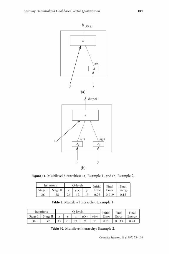
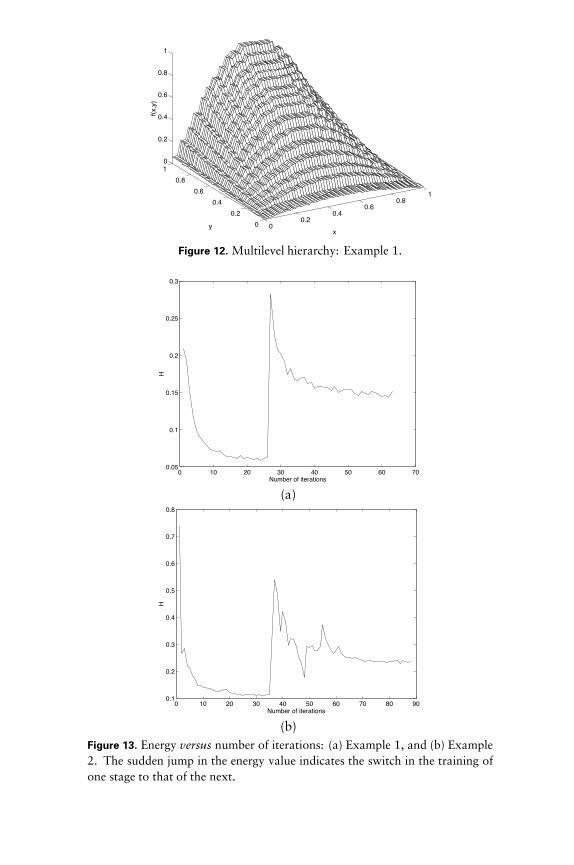
Example 1. The hierarchy is as shown in Figure 11(a). The hierarchyhas a single subordinate-superior pair, and is similar to the single-agentsingle-supervisor case considered previously except for two differences.First, the agent A not only quantizes its environmentx, but also evaluatesits input-output map g($) on the environment x and sends the quantizedoutcome to the supervisor. Second, S, in addition to receiving messagesfrom A, observes its own local environment y. The desired outcomefunction is f (x, y).

Here we take

g(x) = sin(p $ x)f (x, y) = y $ g(x). (5.1)

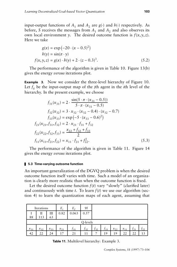
The performance of the algorithm is given in Table 9. Figures 12 and13(a) give, respectively, the output and the energy versus iterations plotof the algorithm.

Example 2. The hierarchy is as shown in Figure 11(b). The hierarchyis similar to that of Example 1 except that now two agents A1 and A2,observing variables x and z respectively, report to supervisor S. The



f(x,y)

S

A

g(x)

xy

(a)

S

z

x y

f(x,y,z)

A A21

h(y)g(x)

(b)

Figure 11. Multilevel hierarchies: (a) Example 1, and (b) Example 2.

Iterations Q-levels Initial Final FinalStage I Stage II x g(x) y Error Error Energy

26 38 24 12 13 0.23 0.019 0.15

Table 9. Multilevel hierarchy: Example 1.

Iterations Q-levels Initial Final FinalStage I Stage II x y z g(x) h(y) Error Error Energy

36 52 17 20 21 9 11 0.73 0.033 0.24



00.2

0.40.6

0.81

00.2

0.40.6

0.810

0.2

0.4

0.6

0.8

1

xy

f(x,y

)

Figure 12. Multilevel hierarchy: Example 1.

0 10 20 30 40 50 60 700.05

0.1

0.15

0.2

0.25

0.3


H

(a)

0 10 20 30 40 50 60 70 80 900.1

0.2

0.3

0.4

0.5

0.6

0.7

0.8


H

(b)Figure 13. Energy versus number of iterations: (a) Example 1, and (b) Example2. The sudden jump in the energy value indicates the switch in the training ofone stage to that of the next.


input-output functions of A1 and A2 are g($) and h($) respectively. Asbefore, S receives the messages from A1 and A2 and also observes itsown local environment y. The desired outcome function is f (x, y, z).Here we take

g(x) = exp I-20 $ (x - 0.5)2Mh(y) = sin(p $ y)

f (x, y, z) = g(x) $ h(y) + 2 $ (z - 0.3)3. (5.2)

The performance of the algorithm is given in Table 10. Figure 13(b)gives the energy versus iterations plot.

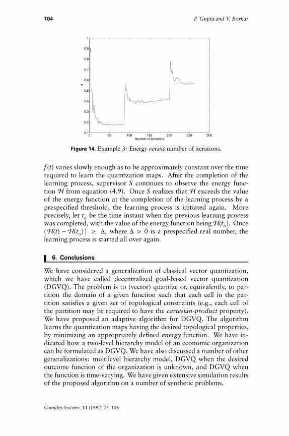
Example 3. Now we consider the three-level hierarchy of Figure 10.Let fij be the input-output map of the jth agent in the ith level of thehierarchy. In the present example, we choose

f31(x31) = 2 $sin(5 $ p $ (x31 - 0.5))

5 $ p $ (x31 - 0.5)f32(x32) = 3 $ x32 $ (x32 - 0.4) $ (x32 - 0.7)f33(x33) = exp I-5 $ (x33 - 0.6)2M

f21(x21, f31, f32) = 2 $ x21 $ f31 + f32

f22(x22, f32, f33) =x22 + f32 + f33

2f11(x11, f21, f22) = x11 $ f21 + f 2

22. (5.3)

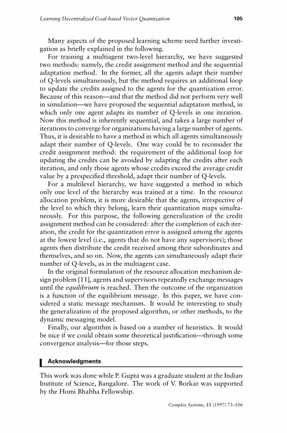
The performance of the algorithm is given in Table 11. Figure 14gives the energy versus iterations plot.

5.3 Time-varying outcome function

An important generalization of the DGVQ problem is when the desiredoutcome function itself varies with time. Such a model of an organiza-tion is clearly more realistic than when the outcome function is fixed.

Let the desired outcome function f (t) vary “slowly” (clarified later)and continuously with time t. To learn f (t) we use our algorithm (sec-tion 4) to learn the quantization maps of each agent, assuming that

Iterations Ei Ef H

I II III 0.82 0.063 0.5788 113 63

Q-levels

x31 x32 x33 x21 f31 f32 f32 f33 x22 x11 f21 f22

42 22 24 17 21 11 7 19 19 22 22 13




0 50 100 150 200 250 3000.1

0.2

0.3

0.4

0.5

0.6

0.7

0.8

0.9

1


H

Figure 14. Example 3: Energy versus number of iterations.

f (t) varies slowly enough as to be approximately constant over the timerequired to learn the quantization maps. After the completion of thelearning process, supervisor S continues to observe the energy func-tion H from equation (4.9). Once S realizes that H exceeds the valueof the energy function at the completion of the learning process by aprespecified threshold, the learning process is initiated again. Moreprecisely, let to be the time instant when the previous learning processwas completed, with the value of the energy function beingH(to). Once(H(t) - H(to) ) % D, where D > 0 is a prespecified real number, thelearning process is started all over again.

6. Conclusions

We have considered a generalization of classical vector quantization,which we have called decentralized goal-based vector quantization(DGVQ). The problem is to (vector) quantize or, equivalently, to par-tition the domain of a given function such that each cell in the par-tition satisfies a given set of topological constraints (e.g., each cell ofthe partition may be required to have the cartesian-product property).We have proposed an adaptive algorithm for DGVQ. The algorithmlearns the quantization maps having the desired topological properties,by minimizing an appropriately defined energy function. We have in-dicated how a two-level hierarchy model of an economic organizationcan be formulated as DGVQ. We have also discussed a number of othergeneralizations: multilevel hierarchy model, DGVQ when the desiredoutcome function of the organization is unknown, and DGVQ whenthe function is time-varying. We have given extensive simulation resultsof the proposed algorithm on a number of synthetic problems.



Many aspects of the proposed learning scheme need further investi-gation as briefly explained in the following.

For training a multiagent two-level hierarchy, we have suggestedtwo methods: namely, the credit assignment method and the sequentialadaptation method. In the former, all the agents adapt their numberof Q-levels simultaneously, but the method requires an additional loopto update the credits assigned to the agents for the quantization error.Because of this reason—and that the method did not perform very wellin simulation—we have proposed the sequential adaptation method, inwhich only one agent adapts its number of Q-levels in one iteration.Now this method is inherently sequential, and takes a large number ofiterations to converge for organizations having a large number of agents.Thus, it is desirable to have a method in which all agents simultaneouslyadapt their number of Q-levels. One way could be to reconsider thecredit assignment method: the requirement of the additional loop forupdating the credits can be avoided by adapting the credits after eachiteration, and only those agents whose credits exceed the average creditvalue by a prespecified threshold, adapt their number of Q-levels.

For a multilevel hierarchy, we have suggested a method in whichonly one level of the hierarchy was trained at a time. In the resourceallocation problem, it is more desirable that the agents, irrespective ofthe level to which they belong, learn their quantization maps simulta-neously. For this purpose, the following generalization of the creditassignment method can be considered: after the completion of each iter-ation, the credit for the quantization error is assigned among the agentsat the lowest level (i.e., agents that do not have any supervisors); thoseagents then distribute the credit received among their subordinates andthemselves, and so on. Now, the agents can simultaneously adapt theirnumber of Q-levels, as in the multiagent case.

In the original formulation of the resource allocation mechanism de-sign problem [11], agents and supervisors repeatedly exchange messagesuntil the equilibrium is reached. Then the outcome of the organizationis a function of the equilibrium message. In this paper, we have con-sidered a static message mechanism. It would be interesting to studythe generalization of the proposed algorithm, or other methods, to thedynamic messaging model.

Finally, our algorithm is based on a number of heuristics. It wouldbe nice if we could obtain some theoretical justification—through someconvergence analysis—for those steps.

Acknowledgments

This work was done while P. Gupta was a graduate student at the IndianInstitute of Science, Bangalore. The work of V. Borkar was supportedby the Homi Bhabha Fellowship.



References

[1] S. C. Ahalt, A. K. Krishnamurthy, P. Chen, and D. Melton, “Competi-tive Learning Algorithms for Vector Quantization,” Neural Networks, 3(1990) 277–290.

[2] D. DeSieno, “Adding a Conscience to Competitive Learning,” in Instituteof Electrical and Electronic Engineers International Conference on NeuralNetworks, (1988) I117–I124.

[3] B. Fritzke, “Growing Cell Structures—A Self-organizing Network for Un-supervised and Supervised Learning,” International Computer ScienceInstitute, Technical Report TR-93-026, Berkeley, 1993.

[4] A. Gersho and R. M. Gray, Vector Quantization and Signal Processing(Kluwer, Boston, 1992).

[5] R. M. Gray, “Vector Quantization,” Institute of Electrical and ElectronicEngineers Acoustics, Speech and Signal Processing Magazine, 1(2) (1984)4–29.

[6] S. Grossberg, “Competitive Learning: From Interactive Activation toAdaptive Resonance,” Cognitive Science, 11 (1987) 23–63.

[7] L. Hurwicz and T. Marschak, “Approximating a Function by choosing aCovering of its Domain and k points from its Range,” Journal of Com-plexity, 4 (1988) 137–174.

[8] T. Kohonen, Self-organization and Associative Memory (second edition,Springer-Verlag, Berlin, 1988).

[9] Y. Linde, A. Buzo, and R. M. Gray, “An Algorithm for Vector Quantiza-tion Design,” Institute of Electrical and Electronic Engineers Transactionson Communications, 28(1) (1980) 84–95.

[10] S. P. Lloyd, “Least-square Quantization in PCM,” Institute of Electri-cal and Electronic Engineers Transactions on Information Theory, 28(2)(1982) 129–137.

[11] T. Marschak, and S. Reichelstein, “Communication Requirements for In-dividual Agents in Networks and Hierarchies,” in The Economics of In-formation Decentralization: Complexity, Efficiency and Stability, editedby J. Ledyard (Kluwer, Boston, 1993).

[12] J. S. Rodrigues and L. B. Almeida, “Improving the Speed in Topolog-ical Maps of Patterns,” Proceedings of International Neural NetworksConference (Paris, 1990).

[13] S. Sathiya Keerthi and B. Ravindran, “A Tutorial Survey of Reinforce-ment Learning,” SADHANA: Indian Academy of Science Proceedings inEngineering Sciences, 19 (1994) 851–889.


Documents

Learning Decentralized Goal-based Vector · PDF fileLearning Decentralized Goal-based Vector Quantization ... From rate distortion theory, ... Learning Decentralized Goal-based Vector