Learning Deep Generative Models - Carnegie Mellon …rsalakhu/papers/annrev.pdf · Recently, Hinton et al. (2006) introduced a moderately fast, unsupervised learning algorithm for

ST02CH15-Salakhutdinov ARI 14 March 2015 8:3

Learning Deep GenerativeModelsRuslan SalakhutdinovDepartments of Computer Science and Statistical Sciences, University of Toronto,Toronto M5S 3G4, Canada; email: [email protected]

Annu. Rev. Stat. Appl. 2015. 2:361–85

The Annual Review of Statistics and Its Application isonline at statistics.annualreviews.org

This article’s doi:10.1146/annurev-statistics-010814-020120

Copyright c© 2015 by Annual Reviews.All rights reserved

Keywords

deep learning, deep belief networks, deep Boltzmann machines, graphicalmodels

Abstract

Building intelligent systems that are capable of extracting high-level rep-resentations from high-dimensional sensory data lies at the core of solv-ing many artificial intelligence–related tasks, including object recognition,speech perception, and language understanding. Theoretical and biologicalarguments strongly suggest that building such systems requires models withdeep architectures that involve many layers of nonlinear processing. In thisarticle, we review several popular deep learning models, including deep beliefnetworks and deep Boltzmann machines. We show that (a) these deep gen-erative models, which contain many layers of latent variables and millions ofparameters, can be learned efficiently, and (b) the learned high-level featurerepresentations can be successfully applied in many application domains, in-cluding visual object recognition, information retrieval, classification, andregression tasks.

361

Ann

ual R

evie

w o

f St

atis

tics

and

Its

App

licat

ion

2015

.2:3

61-3

85. D

ownl

oade

d fr

om w

ww

.ann

ualr

evie

ws.

org

Acc

ess

prov

ided

by

Uni

vers

ity o

f T

oron

to L

ibra

ry o

n 04

/20/

15. F

or p

erso

nal u

se o

nly.


1. INTRODUCTION

Extraction of meaningful representations from rich sensory input lies at the core of solving manyartificial intelligence (AI)-related tasks, including visual object recognition, speech perception,and language comprehension. Theoretical and biological arguments strongly suggest that build-ing such systems requires deep architectures—models composed of several layers of nonlinearprocessing.

Many existing machine learning algorithms use what are called shallow architectures, includingneural networks with only one hidden layer, kernel regression, and support vector machines,among many others. Theoretical results show that the internal representations learned by suchsystems are necessarily simple and are incapable of extracting certain types of complex structurefrom rich sensory input (Bengio & LeCun 2007, Bengio 2009). Training these systems also requireslarge amounts of labeled training data. By contrast, it appears that, for example, object recognitionin the visual cortex uses many layers of nonlinear processing and requires very little labeled input(Lee et al. 1998). Thus, development of new and efficient learning algorithms for models withdeep architectures that can also make efficient use of a large supply of unlabeled sensory input isof crucial importance.

In general, models with deep architectures, including multilayer neural networks, are com-posed of several layers of parameterized nonlinear modules, so the associated loss functions arealmost always nonconvex. The presence of many bad local optima or plateaus in the loss func-tion makes deep models far more difficult to optimize in comparison with shallow models. Localgradient-based optimization algorithms, such as the backpropagation algorithm (Rumelhart et al.1986), require careful parameter initialization and can often get trapped in a poor local optimum,particularly when training models with more than two or three layers (Sutskever et al. 2013). Bycontrast, models with shallow architectures (e.g., support vector machines) generally use convexloss functions, typically allowing one to carry out parameter optimization efficiently. The appealof convexity has steered most machine learning research into developing learning algorithms thatcan be cast in terms of solving convex optimization problems.

Recently, Hinton et al. (2006) introduced a moderately fast, unsupervised learning algorithmfor deep generative models called deep belief networks (DBNs). DBNs are probabilistic graphicalmodels that contain multiple layers of hidden variables. Each nonlinear layer captures progressivelymore complex patterns of data, which represents a promising way of solving problems associatedwith visual object recognition, language comprehension, and speech perception (Bengio 2009).A key feature of the new learning algorithm for DBNs is its layer-by-layer training, which canbe repeated several times to efficiently learn a deep, hierarchical probabilistic model. The newlearning algorithm has excited many researchers in the machine learning community, primarilybecause of the following three crucial characteristics:

1. The greedy layer-by-layer learning algorithm can find a good set of model parametersfairly quickly, even for models that contain many layers of nonlinearities and millions ofparameters.

2. The learning algorithm can make efficient use of very large sets of unlabeled data, so themodel can be pretrained in a completely unsupervised fashion. The very limited labeleddata can then be used to only slightly fine-tune the model for a specific task at hand usingstandard gradient-based optimization.

3. There is an efficient way of performing approximate inference, which makes the values ofthe latent variables in the deepest layer easy to infer.

The strategy of layerwise unsupervised training followed by supervised fine-tuning allowsefficient training of deep networks and gives promising results for many challenging learning

362 Salakhutdinov

Ann

ual R

evie

w o

f St

atis

tics

and

Its

App

licat

ion

2015

.2:3

61-3

85. D

ownl

oade

d fr

om w

ww

.ann

ualr

evie

ws.

org

Acc

ess

prov

ided

by

Uni

vers

ity o

f T

oron

to L

ibra

ry o

n 04

/20/

15. F

or p

erso

nal u

se o

nly.


problems, substantially improving upon the current state of the art (Hinton et al. 2012, Krizhevskyet al. 2012). Many variants of this model have been successfully applied not only for classificationtasks (Hinton et al. 2006, Bengio et al. 2007, Larochelle et al. 2009), but also for regressiontasks (Salakhutdinov & Hinton 2008), visual object recognition (Krizhevsky et al. 2012, Leeet al. 2009, Ranzato et al. 2008), speech recognition (Hinton et al. 2012, Mohamed et al.2012), dimensionality reduction (Hinton & Salakhutdinov 2006, Salakhutdinov & Hinton 2007),information retrieval (Torralba et al. 2008, Salakhutdinov & Hinton 2009c, Uria et al. 2014),natural language processing (Collobert & Weston 2008, Socher et al. 2011, Wang et al. 2012),extraction of optical flow information (Memisevic & Hinton 2010), prediction of quantitativestructure–activity relationships (QSARs) (Dahl et al. 2014), and robotics (Lenz et al. 2013).

Another key advantage of these models is that they are able to capture nonlinear distributedrepresentations. This is in sharp contrast to traditional probabilistic mixture-based latent variablemodels, including topic models (Hofmann 1999, Blei 2014) that are often used to analyze andextract semantic topics from large text collections. Many of the existing topic models, includinga popular Bayesian admixture model, latent Dirichlet allocation (Blei et al. 2003), are based onthe assumption that each document is represented as a mixture of topics, and each topic definesa probability distribution over words. All of these models can be viewed as graphical models inwhich latent topic variables have directed connections to observed variables that represent wordsin a document. One major drawback is that exact inference in these models is intractable, so onehas to resort to slow or inaccurate approximations to compute the posterior distribution overtopics. A second major drawback, which is shared by all mixture models, is that these modelscan never make predictions for words that are sharper than the distributions predicted by any ofthe individual topics. They are unable to capture the essential idea of distributed representations,namely that the distributions predicted by individual active features get multiplied together (andrenormalized) to give the distribution predicted by a whole set of active features. This allowsindividual features to be fairly general but their intersection to be much more precise. For example,distributed representations allow the topics “government,” “mafia,” and “playboy” to combine togive very high probability to the word “Berlusconi,” which is not predicted nearly as stronglyby each topic alone. As shown by Welling et al. (2005) and Salakhutdinov & Hinton (2009b),models that use nonlinear distributed representations are able to generalize much better thanlatent Dirichlet allocation in terms of both the log-probability on previously unseen data vectorsand the retrieval accuracy.

In this article, we provide a general overview of many popular deep learning models, includingdeep belief networks (DBNs) and deep Boltzmann machines (DBMs). In Section 2, we introducerestricted Boltzmann machines (RBMs), which form component modules of DBNs and DBMs,as well as their generalizations to exponential family models. In Section 3, we discuss DBNsand provide a thorough technical review of the greedy learning algorithm for DBNs. Section 4focuses on new learning algorithms for a different type of hierarchical probabilistic model, theDBM. Finally, Section 5 presents a multimodal DBM that can extract a unified representation bylearning a joint density model over the space of multimodal inputs (e.g., images and text, or videoand sound).

2. RESTRICTED BOLTZMANN MACHINESAND THEIR GENERALIZATIONS

Restricted Boltzmann machines (RBMs) have been used effectively in modeling distributions overbinary-valued data. Recent work on Boltzmann machines and their generalizations to exponentialfamily distributions (Welling et al. 2005) have allowed these models to be successfully used in

www.annualreviews.org • Deep Learning 363

Ann

ual R

evie

w o

f St

atis

tics

and

Its

App

licat

ion

2015

.2:3

61-3

85. D

ownl

oade

d fr

om w

ww

.ann

ualr

evie

ws.

org

Acc

ess

prov

ided

by

Uni

vers

ity o

f T

oron

to L

ibra

ry o

n 04

/20/

15. F

or p

erso

nal u

se o

nly.


h

v

W

Figure 1Restricted Boltzmann machine. The top layer represents a vector of “hidden” stochastic binary variables h,and the bottom layer represents a vector of “visible” stochastic binary variables v.

many application domains. In addition to reviewing standard RBMs, this section also reviewsGaussian–Bernoulli RBMs suitable for modeling real-valued inputs for image classification andspeech recognition tasks (Lee et al. 2009, Taylor et al. 2010, Mohamed et al. 2012), as well as thereplicated softmax model (Salakhutdinov & Hinton 2009b), which have been used for modelingsparse count data, such as word count vectors in a document. These models serve as our buildingblocks for other hierarchical models, including DBNs and DBMs.

2.1. Binary Restricted Boltzmann Machines

An RBM is a particular type of Markov random field that has a two-layer architecture (Smolensky1986), in which the “visible” stochastic binary variables v ∈ {0, 1}D are connected to “hidden”stochastic binary variables h ∈ {0, 1}F , as shown in Figure 1. The energy of the joint state {v, h}is defined as follows:

E(v, h; θ ) = −v�W h − b�v − a�h

= −D∑

i=1

F∑j=1

Wi j vi h j −D∑

i=1

bivi −F∑

j=1

a j h j ,

(1)

where θ = {W , b, a} are the model parameters. Wij represents the symmetric interaction termbetween visible variable i and hidden variable j, and bi and aj are bias terms. The joint distributionover the visible and hidden variables is defined by

P (v, h; θ ) = 1Z(θ )

exp(−E(v, h; θ )), (2)

Z(θ ) =∑

v

∑h

exp(−E(v, h; θ )). (3)

Z(θ ) is known as the partition function or normalizing constant. The model then assigns thefollowing probability to a visible vector v:

P (v; θ ) = 1Z(θ )

∑h

exp (−E(v, h; θ )). (4)

364 Salakhutdinov

Ann

ual R

evie

w o

f St

atis

tics

and

Its

App

licat

ion

2015

.2:3

61-3

85. D

ownl

oade

d fr

om w

ww

.ann

ualr

evie

ws.

org

Acc

ess

prov

ided

by

Uni

vers

ity o

f T

oron

to L

ibra

ry o

n 04

/20/

15. F

or p

erso

nal u

se o

nly.


Because RBMs have a special bipartite structure, the hidden variables can be explicitly marginalizedout, as follows:

P (v; θ ) = 1Z(θ )

∑h

exp(v�W h + b�v + a�h

)= 1

Z(θ )exp(b�v)

F∏j=1

∑h j ∈{0,1}

exp

(a j h j +

D∑i=1

Wi j vi h j

)

= 1Z(θ )

exp(b�v)F∏

j=1

(1 + exp

(a j +

D∑i=1

Wi j vi

)).

(5)

The conditional distributions over hidden variables h and visible vectors v can be easily derivedfrom Equation 2 and are given by the following logistic functions:

P (h|v; θ ) =∏

j

p(h j |v), P (v|h; θ ) =∏

i

p(vi |h), (6)

p(h j = 1|v) = g

(∑i

Wi j vi + a j

), (7)

p(vi = 1|h) = g

⎛⎝∑

j

Wi j h j + bi

⎞⎠ , (8)

where g(x) = 1/(1 + exp(−x)) is the logistic function.Given a set of observations {vn}N

n=1, the derivative of the log-likelihood with respect to themodel parameters Wij is obtained from Equation 4:

1N

N∑n=1

∂ log P (vn; θ )∂Wi j

= EPdata [vi h j ] − EPmodel [vi h j ],

1N

N∑n=1

∂ log P (vn; θ )∂a j

= EPdata [h j ] − EPmodel [h j ],

1N

N∑n=1

∂ log P (vn; θ )∂bi

= EPdata [vi ] − EPmodel [vi ],

(9)

where EPdata [·] denotes an expectation with respect to the data distribution Pdata(h, v; θ ) =P (h|v; θ )Pdata(v), where Pdata(v) = 1

N

∑n δ(v − vn) represents the empirical distribution, and

EPmodel [·] is an expectation with respect to the distribution defined by the model, as in Equation 2.We sometimes refer to EPdata [·] as the data-dependent expectation and to EPmodel [·] as the model’sexpectation.

Exact maximum likelihood learning in this model is intractable because exact computation ofthe expectation EPmodel [·] takes time that is exponential in min{D, F}, i.e., the number of visibleor hidden variables. In practice, learning is done by following an approximation to the gradientof a different objective function, called the Contrastive Divergence (CD) algorithm (Hinton2002):

�W = α(EPdata [vh�] − EPT [vh�]), (10)

where α is the learning rate and PT represents a distribution defined by running a Gibbs chaininitialized at the data for T full steps. The special bipartite structure of RBMs allows for anefficient Gibbs sampler that alternates between sampling the states of the hidden variables


Ann

ual R

evie

w o

f St

atis

tics

and

Its

App

licat

ion

2015

.2:3

61-3

85. D

ownl

oade

d fr

om w

ww

.ann

ualr

evie

ws.

org

Acc

ess

prov

ided

by

Uni

vers

ity o

f T

oron

to L

ibra

ry o

n 04

/20/

15. F

or p

erso

nal u

se o

nly.


independently given the states of the visible variables and vice versa (see Equation 6). SettingT = ∞ recovers maximum likelihood learning. In many application domains, however, the CDlearning with T = 1 (or CD1) has been shown to work quite well (Hinton 2002, Welling et al.2005, Larochelle et al. 2009).

2.2. Gaussian–Bernoulli Restricted Boltzmann Machines

When modeling real-valued vectors, such as pixel intensities of image patches, one can easilyextend RBMs to the Gaussian–Bernoulli variant (Hinton & Salakhutdinov 2006). In particular,consider modeling visible real-valued variables v ∈ R

D, and let h ∈ {0, 1}F be stochastic binaryhidden variables. The energy of the joint state {v, h} of the Gaussian RBM is defined as follows:

E(v, h; θ ) =D∑

i=1

(vi − bi )2

2σ 2i

−D∑

i=1

F∑j=1

Wi j h jvi

σi−

F∑j=1

a j h j , (11)

where θ = {W , a, b, σ 2} are the model parameters.The marginal distribution over the visible vector v takes the following form:

P (v; θ ) =∑

h

exp(−E(v, h; θ ))∫v′

∑h exp(−E(v, h; θ ))dv′ . (12)

From Equation 11, derivation of the following conditional distributions is straightforward:

p(vi = x|h) = 1√2πσi

exp

⎛⎜⎝−

(x − bi − σi

∑j h j Wi j

)2

2σ 2i

⎞⎟⎠ , (13)

p(h j = 1|v) = g

(b j +

∑i

Wi jvi

σi

), (14)

where g(x) = 1/(1+exp(−x)) is the logistic function. Observe that conditioned on the states of thehidden variables (Equation 13), each visible unit is modeled by a Gaussian distribution, the meanof which is shifted by the weighted combination of the hidden unit activations. The derivative ofthe log-likelihood with respect to W takes the following form:

∂ log P (v; θ )∂Wi j

= EPdata

[1σi

vi h j

]− EPmodel

[1σi

vi h j

].

As discussed in Section 2.1, learning of the model parameters, including the variance σ 2, can becarried out using CD. In practice, however, instead of learning σ 2, one would typically use a fixed,predetermined value for σ 2 (Nair & Hinton 2009, Hinton & Salakhutdinov 2006).

Figure 2 shows a random subset of parameters W, also known as receptive fields, learnedby a standard binary RBM and a Gaussian–Bernoulli RBM using Contrastive Divergence CD1.Observe that both RBMs learn highly localized receptive fields.

2.3. Replicated Softmax Model

The replicated softmax model represents another extension of the RBM and is used for modelingsparse count data, such as word count vectors in a document (Salakhutdinov & Hinton 2009b,2013). Consider an undirected graphical model that consists of one visible layer and one hiddenlayer, as shown in Figure 3. This model is a type of RBM in which the visible variables that areusually binary have been replaced by softmax variables, each of which can have one of a numberof different states.

366 Salakhutdinov

Ann

ual R

evie

w o

f St

atis

tics

and

Its

App

licat

ion

2015

.2:3

61-3

85. D

ownl

oade

d fr

om w

ww

.ann

ualr

evie

ws.

org

Acc

ess

prov

ided

by

Uni

vers

ity o

f T

oron

to L

ibra

ry o

n 04

/20/

15. F

or p

erso

nal u

se o

nly.


Training samples Learned receptive fieldsTraining samples Learned receptive fields

a b

Figure 2A random subset of the training images along with the learned receptive fields. (a) The binary restrictedBoltzmann machine (RBM) trained on the Handwritten Characters data set (resolution is 28 × 28). (b) TheGaussian–Bernoulli RBM trained on the CIFAR-100 data set (resolution is 32 × 32). Each square displaysthe incoming weights from all of the visible variables into one hidden unit.

Specifically, let K be the dictionary size, M be the number of words appearing in a document,and h ∈ {0, 1}F be stochastic binary hidden topic features. Let V be an M × K observed binarymatrix with vik = 1 if visible unit i takes on value k (meaning the ith word in the document is thekth dictionary word). The energy of the state {V, h} can be defined as follows:

E(V, h) = −M∑

i=1

F∑j=1

K∑k=1

Wi jkh j vik −M∑

i=1

K∑k=1

vikbik −F∑

j=1

h j a j , (15)

where {W, a, b} are the model parameters. Wijk is a symmetric interaction term between visiblevariable i that takes on value k and hidden variable j, bik is the bias of unit i that takes on valuek, and aj is the bias of hidden feature j. The model assigns the following probability to a visiblebinary matrix V:

P (V ; θ ) = 1Z(θ )

∑h

exp(−E(V, h; θ )), Z(θ ) =∑

V

∑h

exp(−E(V, h; θ )). (16)

Now suppose that for each document, we create a separate RBM with as many softmax unitsas there are words in the document. Assuming we can ignore the order of the words, all of thesesoftmax units can share the same set of weights connecting them to binary hidden units. In thiscase, the energy of the state {V, h} for a document that contains M words is defined as follows:

E(V, h) = −F∑

j=1

K∑k=1

W jkh j vk −K∑

k=1

vkbk − MF∑

j=1

h j a j , (17)

W1

W1 W2

W2

h

v

h

v

W1W1

W1

W2W2

W2

W1 W2

Latent topics Latent topics

a b

Observed softmax visibles Multinomial visible

Figure 3The replicated softmax model. The top layer represents a vector h of stochastic binary hidden topic features, and the bottom layerconsists of softmax visible variables, v. All visible variables share the same set of weights, connecting them to the binary hiddenvariables. (a) Two members of a replicated softmax family for documents containing two and three words. (b) A different interpretationof the replicated softmax model, in which M softmax variables with identical weights are replaced by a single multinomial variable thatis sampled M times.


Ann

ual R

evie

w o

f St

atis

tics

and

Its

App

licat

ion

2015

.2:3

61-3

85. D

ownl

oade

d fr

om w

ww

.ann

ualr

evie

ws.

org

Acc

ess

prov

ided

by

Uni

vers

ity o

f T

oron

to L

ibra

ry o

n 04

/20/

15. F

or p

erso

nal u

se o

nly.


where vk = ∑Mi=1 vk

i denotes the count for the kth word. The bias terms of the hidden units arescaled up by the length of the document. This scaling is crucial and allows hidden units to behavesensibly when dealing with documents of different lengths.

The corresponding conditional distributions are given by the following equations:

p(h j = 1|V ) = g

(M a j +

K∑k=1

vkW jk

), (18)

p(vik = 1|h) =exp

(bk + ∑F

j=1 h j W jk

)∑K

q=1 exp(

bq + ∑Fj=1 h j W jq

) . (19)

We also note that using M softmax variables with identical weights is equivalent to having a singlevisible multinomial variable with support {1, . . . , K } that is sampled M times (see Figure 3b).

A pleasing property of using softmax variables is that the mathematics underlying the learningalgorithm for binary RBMs remains the same. Given a collection of N documents {V n}N

n=1, thederivative of the log-likelihood with respect to parameters W takes the following form:

1N

N∑n=1

∂ log P (Vn)∂W jk

= EPdata [vkh j ] − EPmodel [vkh j ].

Similar to other types of RBMs, learning can be performed using CD.Table 1 shows one-step reconstructions of some bags of words to illustrate what this replicated

softmax model is learning (Srivastava & Salakhutdinov 2014). The model was trained using textfrom the MIR-Flickr data set (Huiskes & Lew 2008). The words in the left column were presentedas input to the model, after which Equation 18 was used to compute a distribution over hiddenunits. Taking these probabilities as the states of the hidden units, Equation 19 was used to obtain adistribution over words. The right column shows the words with the highest probabilities in thatdistribution. Observe that the model has learned a reasonable notion of semantic similarity. Forexample, “chocolate, cake” generalizes to “sweets, desserts, food.” Note that the model is able tocapture some regularities about language, discover synonyms across multiple languages, and learnabout geographical relationships.

3. DEEP BELIEF NETWORKS

A single layer of binary features is not the best way to capture the structure in high-dimensionalinput data. In this section, we describe an efficient way to learn additional layers of binary featuresusing deep belief networks (DBNs).

Table 1 Some examples of one-step reconstruction from the replicated softmax model

Input Reconstructionchocolate, cake cake, chocolate, sweets, dessert, cupcake, food, sugar, cream, birthdaynyc nyc, newyork, brooklyn, queens, gothamist, manhattan, subway, streetartdog dog, puppy, perro, dogs, pet, filmshots, tongue, pets, nose, animalflower, high, flower, , high, japan, sakura, , blossom, tokyo, lily, cherrygirl, rain, station, norway norway, station, rain, girl, oslo, train, umbrella, wet, railway, weatherfun, life, children children, fun, life, kids, child, playing, boys, kid, play, loveforest, blur forest, blur, woods, motion, trees, movement, path, trail, green, focusespana, agua, granada espana, agua, spain, granada, water, andalucıa, naturaleza, galicia, nieve

368 Salakhutdinov

Ann

ual R

evie

w o

f St

atis

tics

and

Its

App

licat

ion

2015

.2:3

61-3

85. D

ownl

oade

d fr

om w

ww

.ann

ualr

evie

ws.

org

Acc

ess

prov

ided

by

Uni

vers

ity o

f T

oron

to L

ibra

ry o

n 04

/20/

15. F

or p

erso

nal u

se o

nly.


h

v

W(1)

h1

h2

v

W(1)

W(1)

a b

Figure 4(a) A restricted Boltzmann machine (RBM). (b) A two-hidden-layer deep belief network (DBN) with tiedweights W (2) = W (1)� . The joint distribution P (v, h(1); W (1)) defined by this DBN is identical to the jointdistribution P (v, h(1); W (1)) defined by an RBM.

DBNs are probabilistic generative models that contain many layers of hidden variables, inwhich each layer captures high-order correlations between the activities of hidden features in thelayer below. The top two layers of the DBN form an RBM model in which the lower layers forma directed sigmoid belief network, as shown in Figure 4. Hinton et al. (2006) introduced a fastunsupervised learning algorithm for these deep networks. A key feature of their algorithm is itsgreedy layer-by-layer training, which can be repeated several times to learn a deep hierarchicalmodel. The learning procedure also provides an efficient way of performing approximate inference,which only requires a single bottom-up pass to infer the values of the top-level hidden variables.

Let us first consider learning a DBN with two layers of hidden variables {h(1), h(2)}. We alsoassume that the number of second-layer hidden variables is the same as the number of visiblevariables (see Figure 4b). The top two layers of the DBN form an undirected bipartite graph, anRBM, and the lower layers form a directed sigmoid belief network. The joint distribution over v,h(1), and h(2) defined by this model takes the following form:1

P (v, h(1), h(2); θ ) = P (v|h(1); W (1))P (h(1), h(2); W (2)), (20)

where θ = {W (1), W (2)} are the model parameters, P (v|h(1); W (1)) is the directed sigmoid beliefnetwork, and P (h(1), h(2); W (2)) is the joint distribution defined by the second-layer RBM.

P (v|h(1); W (1)) =∏

i

p(vi |h(1); W (1)), p(vi = 1|h(1); W (1)) = g

⎛⎝∑

j

W (1)i j h(1)

j

⎞⎠ , (21)

P (h(1), h(2); W (2)) = 1Z(W (2))

exp(h(1)� W (2)h(2)), (22)

where g(x) = 1/(1 + exp(−x)) is the logistic function.The greedy layer-by-layer learning strategy relies on the following key observation. Consider

a two-hidden-layer DBN with tied parameters W (2) = W (1)� . The joint distribution of this DBN,P (v, h(1); θ ) = ∑

h(2) P (v, h(1), h(2); θ ), is identical to the joint distributionP (v, h(1); W (1)) of theRBM (see Equation 2). Indeed, one can easily see from Figure 4 that the marginal distribution overh(1), P (h(1); W (1)) is the same for both models. Similarly, the conditional distribution P (v|h(1); W (1))is also the same for both models. To be more precise, using Equations 20–22 and the fact that

1We omit the bias terms here for clarity of presentation.


Ann

ual R

evie

w o

f St

atis

tics

and

Its

App

licat

ion

2015

.2:3

61-3

85. D

ownl

oade

d fr

om w

ww

.ann

ualr

evie

ws.

org

Acc

ess

prov

ided

by

Uni

vers

ity o

f T

oron

to L

ibra

ry o

n 04

/20/

15. F

or p

erso

nal u

se o

nly.


W (2) = W (1)� , we obtain the following joint distribution over {v, h(1)} of the DBN:

P (v, h(1); θ ) = P (v|h(1); W (1)) ×∑h(2)

P (h(1), h(2); W (2))

=∏

i

p(vi |h(1); W (1)) × 1Z(W (2))

∏i

⎛⎝1 + exp

⎛⎝∑

j

W (2)j i h(1)

j

⎞⎠

⎞⎠

=∏

i

exp(vi

∑j W (1)

i j h(1)j

)1 + exp

(∑j W (1)

i j h(1)j

) × 1Z(W (2))

∏i

⎛⎝1 + exp

⎛⎝∑

j

W (2)j i h(1)

j

⎞⎠

⎞⎠

= 1Z(W (1))

∏i

⎛⎝exp

⎛⎝vi

∑j

W (1)i j h(1)

j

⎞⎠

⎞⎠[

because W (2)j i = W (1)

i j ,Z(W (1)) = Z(W (2))]

= 1Z(W (1))

exp

⎛⎝∑

i j

W (1)i j vi h

(1)j

⎞⎠ , (23)

which is identical to the joint distribution over {v, h(1)} defined by an RBM (Equation 2).The greedy learning algorithm uses a stack of RBMs (see Figure 5) and proceeds as follows.

We first train the bottom RBM with parameters W (1) as described in Section 2. We then initializethe second layer weights to W (2) = W (1)� , ensuring that the two-hidden-layer DBN is at leastas good as our original RBM. We can now improve the fit of the DBN to the training data byuntying and refitting parameters W (2).

For any approximating distribution Q(h(1)|v) [provided that Q(h(1)|v) �= 0 wheneverP (v, h(1); θ ) �= 0], the log-likelihood of the two-hidden-layer DBN model has the following

RBM

RBM

RBM

Deep belief network

ba

Figure 5(a) Greedy learning of a stack of restricted Boltzmann machines (RBMs) in which the samples from thelower-level RBM are used as the data for training the next RBM. (b) The corresponding deep belief network.

370 Salakhutdinov

Ann

ual R

evie

w o

f St

atis

tics

and

Its

App

licat

ion

2015

.2:3

61-3

85. D

ownl

oade

d fr

om w

ww

.ann

ualr

evie

ws.

org

Acc

ess

prov

ided

by

Uni

vers

ity o

f T

oron

to L

ibra

ry o

n 04

/20/

15. F

or p

erso

nal u

se o

nly.


variational lower bound, where the states h(2) are analytically summed out:

log P (v; θ ) = log∑h(1)

P (v, h(1); θ ) = log∑h(1)

Q(h(1)|v)P (v, h(1); θ )

Q(h(1)|v)

≥∑h(1)

Q(h(1)|v)[

logP (v, h(1); θ )

Q(h(1)|v)

]( Jensen’s inequality)

=∑h(1)

Q(h(1)|v)[log P (v, h(1); θ )

] +∑h(1)

Q(h(1)|v)[

log1

Q(h(1)|v)

]

=∑h(1)

Q(h(1)|v)[log P (h(1); W (2)) + log P (v|h(1); W (1))

] + H (Q(h(1)|v)),

(24)

where H(·) is the entropy functional. We set Q(h(1)|v) = P (h(1)|v; W (1)), as defined by the bottomRBM (Equation 6). Initially, when W (2) = W (1)� , Q is the true factorial posterior over h(1) of theDBN, in which case the bound is tight. The strategy of the greedy learning algorithm is to fixthe parameter vector W (1) and attempt to learn a better model for P (h(1); W (2)) by maximizingthe variational lower bound of Equation 24 with respect to W (1). Maximizing this bound withfixed W (1) amounts to maximizing∑

h(1)

Q(h(1)|v) log P (h(1); W (2)), (25)

which is equivalent to maximum likelihood training of the second-layer RBM with vectors h(1)

drawn from Q(h(1)|v) as data. When presented with a data set of N training input vectors, thesecond-layer RBM, P (h(1); W (2)), will learn a better model of the aggregated posterior over h(1),which is simply the mixture of factorial posteriors for all the training cases, 1

N

∑n P (h(1)|vn; W (1)).

Note that any increase in the variational lower bound that results from changing W (2) will alsoresult in an increase of the data likelihood of the DBN.2

Algorithm 1 (Recursive greedy learning procedure for the deep belief network):

1: Fit the parameters W (1) of the first-layer RBM to data.2: Fix the parameter vector W (1), and use samples h(1) from Q(h(1)|v) = P (h(1)|v, W (1))as the data for training the next layer of binary features with an RBM.3: Fix the parameters W (2) that define the second layer of features, and use the samplesh(2) from Q(h(2)|h(1)) = P (h(2)|h(1), W (2)) as the data for training the third layer of binaryfeatures.4: Proceed recursively for the next layers.

This idea can be extended to training the third-layer RBM on vectors h(2) drawn from thesecond-layer RBM. By initializing W (3) = W (2)� , we are guaranteed to improve the lower boundon the log-likelihood, although changing W (3) to improve the bound can decrease the actuallog-likelihood. This greedy layer-by-layer training can be repeated several times to learn a deephierarchical model. The procedure is summarized in Algorithm 1.

2Improving the variational bound by changing W (2) will increase the log-likelihood because the bound is initially tight.When learning deeper layers, the variational bound is not initially tight, so even the initial improvement in the bound is notguaranteed to increase the log-likelihood.


Ann

ual R

evie

w o

f St

atis

tics

and

Its

App

licat

ion

2015

.2:3

61-3

85. D

ownl

oade

d fr

om w

ww

.ann

ualr

evie

ws.

org

Acc

ess

prov

ided

by

Uni

vers

ity o

f T

oron

to L

ibra

ry o

n 04

/20/

15. F

or p

erso

nal u

se o

nly.


...h2 ~ P(h2,h3)

h1 ~ P(h1|h2)

v ~ P(v|h1)

h3 ~ Q(h3|h2)

h2 ~ Q(h2|h1)

h1 ~ Q(h1|v)

v

h3 ~ Q(h3|v)

h2 ~ Q(h2|v)

h1 ~ Q(h1|v)

v

Gibbs chaina b~

~

~

Figure 6(a) Sample generation from the deep belief network. (b) Sample generation from approximate posteriorQ(h(1), h(2), h(3)|v) (left) versus from fully factorized approximate posterior Q(h(1)|v)Q(h(2)|v)Q(h(3)|v) (right).

Algorithm 2 (Modified recursive greedy learning procedure for the deep beliefnetwork):

1: Fit the parameters W (1) of the first-layer RBM to data.2: Fix the parameter vector W (1), and use samples h(1) from Q(h(1)|v) = P (h(1)|v, W (1))as the data for training the next layer of binary features with an RBM.3: Fix the parameters W (2) that define the second layer of features, and use the samplesh(2) from Q(h(2)|v) as the data for training the third layer of binary features.4: Proceed recursively for the next layers.

After training a DBN with L layers, the joint distribution of the model P and its approximateposterior distribution Q are given by:

P (v, h(1), . . . , h(L)) = P (v|h(1)) . . . P (h(L−2)|h(L−1))P (h(L−1), h(L)),

Q(h(1), . . . , h(L)|v) = Q(h(1)|v)Q(h(2)|h(1)) . . . Q(h(L)|h(L−1)).

To generate an approximate sample from the DBN, we can run an alternating Gibbs sampler(Equation 6) to generate an approximate sample h(L−1) from P (h(L−1), h(L)), defined by the top-level RBM, followed by a top-down pass through the sigmoid belief network by stochasticallyactivating each lower layer in turn (see Figure 6a). To get a sample from the approximate poste-rior distribution Q, we simply perform a bottom-up pass by stochastically activating each higherlayer in turn. The marginal distribution of the top-level hidden variables of our approximateposterior Q(h(L)|v) will be nonfactorial and, in general, could be multimodal. For many practicalapplications (e.g., information retrieval), having an explicit form for Q(h(L)|v), which allows ef-ficient approximate inference, is of crucial importance. One possible alternative is to choose thefollowing fully factorized approximating distribution Q:

Q(h(1), . . . , h(L)|v) =L∏

l=1

Q(h(l)|v), (26)

where we define

Q(h(1)|v) =∏

j

q (h(1)j |v), q (h(1)

j = 1|v) = g

(∑i

W (1)i j vi + a (1)

j

), and (27)

Q(h(l)|v) =∏

j

q (h(l)j |v), q (h(l)

j = 1|v) = g

(∑i

W (l)i j q (h(l−1)

i = 1|v) + a (l)j

), (28)

372 Salakhutdinov

Ann

ual R

evie

w o

f St

atis

tics

and

Its

App

licat

ion

2015

.2:3

61-3

85. D

ownl

oade

d fr

om w

ww

.ann

ualr

evie

ws.

org

Acc

ess

prov

ided

by

Uni

vers

ity o

f T

oron

to L

ibra

ry o

n 04

/20/

15. F

or p

erso

nal u

se o

nly.


where g(x) = 1/(1 + exp(−x)) and l = 2, . . . , L. The factorial posterior Q(h(L)|v) is obtainedby simply replacing the stochastic hidden variables with real-valued probabilities and then per-forming a single deterministic bottom-up pass to compute q (h(L)

j = 1|v). This fully factorizedapproximation also suggests a modified greedy learning algorithm, summarized in Algorithm 2.In this modified algorithm, the samples used for training higher-level RBMs are instead taken froma fully factorized approximate posterior Q. Note that the modified algorithm does not guaranteeto improve the lower bound on the log-probability of the training data. Nonetheless, this is theactual algorithm commonly used in practice (Hinton & Salakhutdinov 2006, Taylor et al. 2006,Torralba et al. 2008, Bengio 2009). The modified algorithm works well, particularly when a fullyfactorized Q is used to perform approximate inference in the final model.

DBNs can also be used for classification and regression tasks. Many of the resulting extensionsexploit the following two key properties of DBNs. First, they can be learned efficiently from largeamounts of unlabeled data. Second, they can be discriminatively fine-tuned using the standardbackpropagation algorithm. For example, a DBN can be used to extract useful feature representa-tions that allow one to learn a good covariance kernel for a Gaussian process model (Salakhutdinov& Hinton 2008). The greedy learning algorithm can also be used to make nonlinear autoencoderswork considerably better than widely used methods, such as principal component analysis (PCA)and singular value decomposition (SVD) (Hinton & Salakhutdinov 2006). Similarly, layer-by-layer pretraining followed by discriminative fine-tuning achieves good performance on phonerecognition tasks, as well as on various audio classification tasks (Lee et al. 2009, Taylor et al.2010, Mohamed et al. 2012).

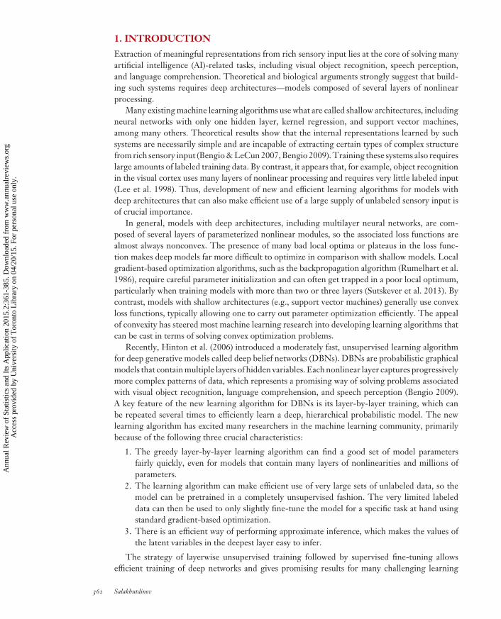
4. DEEP BOLTZMANN MACHINES

In this section we present a new learning algorithm for a different type of hierarchical probabilis-tic model, called a deep Boltzmann machine (DBM). Unlike DBNs, a DBM is a type of Markovrandom field, or undirected graphical model, in which all connections between layers are undi-rected. DBMs are interesting for several reasons. First, similar to DBNs, DBMs have the abilityto learn internal representations that capture complex statistical structure in the higher layers. Ashas already been demonstrated for DBNs, this is a promising way of solving object and speechrecognition problems (Bengio 2009, Bengio & LeCun 2007, Hinton et al. 2006, Mohamed et al.2012). High-level representations are built from a large supply of unlabeled data, and a muchsmaller supply of labeled data can then be used to fine-tune the model for a specific discriminationtask. Second, if DBMs are learned in the right way there is a very fast way to initialize the states ofthe variables in all layers by a simple bottom-up pass. Third, unlike DBNs and many other modelswith deep architectures (Ranzato et al. 2007, Vincent et al. 2008, Serre et al. 2007), the approx-imate inference procedure, after the initial bottom-up pass, can incorporate top-down feedback,allowing DBMs to use higher-level knowledge to resolve uncertainty about intermediate-levelfeatures, thus creating better data-dependent representations, as well as better data-dependentstatistics for learning.

Consider a three-hidden-layer DBM, as shown in Figure 7b, with no within-layer connections.The energy of the state {v, h(1), h(2), h(3)} is defined as

E(v, h(1), h(2), h(3); θ ) = −v�W (1)h(1) − h(1)�W (2)h(2) − h(2)�W (3)h(3), (29)

where θ = {W (1), W (2), W (3)} are the model parameters, representing visible-to-hidden andhidden-to-hidden symmetric interaction terms. The model assigns the following probability to a


Ann

ual R

evie

w o

f St

atis

tics

and

Its

App

licat

ion

2015

.2:3

61-3

85. D

ownl

oade

d fr

om w

ww

.ann

ualr

evie

ws.

org

Acc

ess

prov

ided

by

Uni

vers

ity o

f T

oron

to L

ibra

ry o

n 04

/20/

15. F

or p

erso

nal u

se o

nly.


h(1)

h(2)

h(3)

v

W(3)

W(2)

W(1)

h(1)

h(2)

h(3)

v

W(3)

W(2)

W(1)

Deep belief networka b Deep Boltzmann machine

Figure 7(a) Deep belief network (DBN) in which the top two layers form an undirected graph and the remaininglayers form a belief net with directed, top-down connections. (b) Deep Boltzmann machine (DBM) withvisible-to-hidden and hidden-to-hidden connections, but no within-layer connections. All of the connectionsin a DBM are undirected.

visible vector v:

P (v; θ ) = 1Z(θ )

∑h(1),h(2),h(3)

exp(−E(v, h(1), h(2), h(3); θ )). (30)

Observe that setting both W (2) = 0 and W (3) = 0 recovers the simpler RBM model. The condi-tional distributions over the visible and the three sets of hidden variables are given by the followinglogistic functions:

p(h(1)j = 1|v, h(2)) = g

(∑i

W (1)i j vi +

∑m

W (2)jmh(2)

m

), (31)

p(h(2)m = 1|h(1), h(3)) = g

⎛⎝∑

j

W (2)jmh(1)

j +∑

l

W (3)ml h(3)

l

⎞⎠ , (32)

p(h(3)l = 1|h(2)) = g

(∑m

W (3)ml h(2)

m

), (33)

p(vi = 1|h(1)) = g

⎛⎝∑

j

W (1)i j h(1)

j

⎞⎠ . (34)

The derivative of the log-likelihood with respect to the model parameters takes the followingform:

∂ log P (v; θ )∂W (1)

= EPdata [vh(1)� ] − EPmodel [vh(1)� ], (35)

where EPmodel [·] denotes an expectation with respect to the distribution defined by the model,and EPdata [·] is an expectation with respect to the completed data distribution Pdata(h, v; θ ) =P (h|v; θ )Pdata(v), where Pdata(v) = 1

N

∑n δ(v − vn) represents the empirical distribution. The

derivatives with respect to parameters W (2) and W (3) take similar forms, but they involve theouter products h(1)h(2)� and h(2)h(3)� , respectively. Unlike RBMs, the conditional distribution over

374 Salakhutdinov

Ann

ual R

evie

w o

f St

atis

tics

and

Its

App

licat

ion

2015

.2:3

61-3

85. D

ownl

oade

d fr

om w

ww

.ann

ualr

evie

ws.

org

Acc

ess

prov

ided

by

Uni

vers

ity o

f T

oron

to L

ibra

ry o

n 04

/20/

15. F

or p

erso

nal u

se o

nly.


the states of the hidden variables conditioned on the data is no longer factorial. The exact compu-tation of the data-dependent expectation takes time that is exponential in the number of hiddenvariables, whereas the exact computation of the model’s expectation takes time that is exponentialin the number of hidden and visible variables.

4.1. Approximate Maximum Likelihood Learning

The original learning algorithm for general Boltzmann machines used randomly initializedMarkov chains to approximate both of the expectations needed to approximate gradients of thelikelihood function (Hinton & Sejnowski 1983). This learning procedure is too slow to be practical,however, so we now consider a variational approach to alleviate this problem. In the variationalapproach, mean-field inference is used to estimate data-dependent expectations, and a Markovchain Monte Carlo (MCMC)-based stochastic approximation procedure is used to approximatethe model’s expected sufficient statistics (Tieleman 2008, Salakhutdinov 2008, Salakhutdinov &Hinton 2009a).

Consider any approximating distribution Q(h|v; μ) for the posterior P (h|v; θ ). Similar to theDBN bound given in Equation 24, the DBM’s variational lower bound on the log-likelihood takesthe following form:

log P (v; θ ) ≥∑

h

Q(h|v; μ) log P (v, h; θ ) + H(Q), (36)

whereH(·) is the entropy functional. The bound becomes tight if and only if Q(h|v; μ) = P (h|v; θ ).For simplicity and speed, we approximate the true posterior using a fully factorized distribution

(i.e., the naive mean-field approximation) over the three sets of hidden variables:

QMF(h|v; μ) =F1∏j=1

F2∏k=1

F3∏m=1

q (h(1)j )q (h(2)

k )q (h(3)m ), (37)

where μ = {μ(1), μ(2), μ(3)} are the mean-field parameters with q (hli = 1) = μl

i for l = 1,2,3. Inthis case, the lower bound of Equation 36 takes a particularly simple form:

log P (v; θ ) ≥ v�W (1)μ(1) + μ(1)� W (2)μ(2) + μ(2)� W (3)μ(3)

− logZ(θ ) + H(Q).(38)

Learning proceeds as follows: For each training example, we find the value of μ that maximizesthis lower bound for the current value of θ . This optimum must satisfy the following mean-fieldfixed-point equations:

μ(1)j ← σ

(D∑

i=1

W (1)i j vi +

F2∑k=1

W (2)j k μ

(2)k

), (39)

μ(2)k ← σ

⎛⎝ F1∑

j=1

W (2)j k μ

(1)j +

F3∑m=1

W (3)kmμ(3)

m

⎞⎠ , (40)

μ(3)m ← σ

( F2∑k=1

W (3)kmμ

(2)k

). (41)

Note the close connection between the form of the mean-field fixed-point updates and theform of the conditional distributions defined by Equations 31–33.3 To solve these fixed-point

3Implementing the mean-field requires no extra work beyond implementing the Gibbs sampler.


Ann

ual R

evie

w o

f St

atis

tics

and

Its

App

licat

ion

2015

.2:3

61-3

85. D

ownl

oade

d fr

om w

ww

.ann

ualr

evie

ws.

org

Acc

ess

prov

ided

by

Uni

vers

ity o

f T

oron

to L

ibra

ry o

n 04

/20/

15. F

or p

erso

nal u

se o

nly.


equations, we simply cycle through layers, updating the mean-field parameters within a singlelayer. The variational parameters μ are then used to compute the data-dependent statistics inEquation 35. For example,

EPdata [vh(1)� ] = 1N

N∑n=1

vnμ(1)�n

EPdata [h(1)h(2)� ] = 1

N

N∑n=1

μ(1)n μ(2)�

n ,

where the averages are taken over the training cases.Given the variational parameters μ, the model parameters θ are then updated to maximize

the variational bound using an MCMC-based stochastic approximation (Younes 2000, Tieleman2008, Salakhutdinov & Hinton 2009a). In particular, let θt and xt = {v, h(1), h(2)} be the currentparameters and the state, respectively. Then xt and θ t are updated sequentially as follows:

1. Given xt, sample a new state xt+1 from the transition operator T θt (xt+1 ← xt) that leavesP (·; θt) invariant. Sampling this new state is accomplished using Gibbs sampling (seeEquations 31–33).

2. A new parameter θt+1 is then obtained by making a gradient step, in which the intractablemodel’s expectation EPmodel [·] in the gradient is replaced by a point estimate at sample xt+1.

In practice, to reduce the variance of the estimator, we typically maintain a set of S Markovchains X t = {xt,1, . . . , xt,S} and use an average over those particles.

Stochastic approximation provides asymptotic convergence guarantees and belongs to the gen-eral class of Robbins–Monro approximation algorithms (Robbins & Monro 1951, Younes 2000).Sufficient conditions that ensure almost sure convergence to an asymptotically stable point aregiven in articles by Younes (1989, 2000) and Yuille (2004). One necessary condition requires thelearning rate to decrease with time, such that

∑∞t=0 αt = ∞ and

∑∞t=0 α2

t < ∞. For example, thiscondition can be satisfied by αt = a/(b + t), for positive constants a > 0, b > 0. In practice, thesequence |θt | is typically bounded, and the Markov chain, governed by the transition kernel Tθ , istypically ergodic. Together with the condition on the learning rate, these conditions are sufficientto ensure almost sure convergence of the stochastic approximation algorithm to an asymptoticallystable point (Younes 2000, Yuille 2004).

The learning procedure for DBMs described above can be used by initializing model parametersat random. The model performs much better if parameters are initialized sensibly, however, so itis common to use a greedy layerwise pretraining strategy by learning a stack of RBMs (for details,see Salakhutdinov & Hinton 2009a). The pretraining procedure is quite similar to the one usedfor DBNs discussed in Section 3, and it allows us to perform approximate inference using a singlebottom-up pass. This fast approximate inference can also be used to initialize the mean-field,which then converges much faster than does a mean-field initialized at random.

4.2. Evaluating Deep Boltzmann Machines as Discriminative Models

After learning, the stochastic activities of the binary features in each layer are replaced by deter-ministic, real-valued probabilities, and a DBM with two hidden layers can be used to initialize amultilayer neural network in the following way: For each input vector v, the mean-field inferenceis used to obtain an approximate posterior distribution Q(h(2)|v). The marginals q (h(2)

j = 1|v) ofthis approximate posterior, together with the data, are used to create what we call an augmentedinput for this deep multilayer neural network, as shown in Figure 8. This augmented input is

376 Salakhutdinov

Ann

ual R

evie

w o

f St

atis

tics

and

Its

App

licat

ion

2015

.2:3

61-3

85. D

ownl

oade

d fr

om w

ww

.ann

ualr

evie

ws.

org

Acc

ess

prov

ided

by

Uni

vers

ity o

f T

oron

to L

ibra

ry o

n 04

/20/

15. F

or p

erso

nal u

se o

nly.


v

h(1)

h(2)

W(1)

W(2)

...

vvvv

2W(1) W(1)

W(2) W(2)

Q(h(1))

Q(h(2))

y y

Fine-tune Q(h(2))

W(2) W(1)

W(2)

W(3)Mean-field updatesa b

Figure 8(a) A two-hidden-layer Boltzmann machine. (b) After learning, the deep Boltzmann machine is used toinitialize a multilayer neural network. The marginals of the approximate posterior q (h(2)

j = 1|v) are used asadditional inputs. The network is fine-tuned by backpropagation.

important because it maintains the scale of the inputs that each hidden variable expects. Forexample, the conditional distribution over h(1), as defined by the DBM model (see Equation 31),takes the following form:

p(h(1)j = 1|v, h(2)) = g

(∑i

W (1)i j vi +

∑m

W (2)jmh(2)

m

).

Hence, the layer h(1) receives inputs from both v and h(2). When this DBM is used to initializea feed-forward network (Figure 8b), the augmented inputs Q(h(2)|v) serve as a proxy for h(2),ensuring that when the feed-forward network is fine-tuned using standard backpropagation oferror derivatives, the hidden variables in h(1) initially receive the same input as they would havereceived in a mean-field update during the pretraining stage.

The unusual representation of the input is a by-product of converting a DBM into a determin-istic neural network. In general, the gradient-based fine-tuning may choose to ignore Q(h(2)|v);that is, the fine-tuning may drive the first-layer connections W (2) to zero, resulting in a stan-dard neural network. Conversely, the network may choose to ignore the input by driving thefirst-layer weights W(1) to zero and making its predictions on the basis of only the approximateposterior. However, the network typically makes use of the entire augmented input for makingpredictions.

4.3. Experimental Results

To illustrate the kinds of probabilistic models DBMs are capable of learning, we conducted ex-periments on two well-studied data sets: the MNIST and NORB data sets.

4.3.1. MNIST data set. The Mixed National Institute of Standards and Technology (MNIST)database of handwritten digits contains 60,000 training images and 10,000 test images of tenhandwritten digits (0 to 9), each of which is centered within a 28 × 28 pixel image. Intermediateintensities between 0 and 255 were treated as probabilities, and we sampled binary valuesfrom these probabilities independently for each pixel each time an image was used. In our firstexperiment, we trained two DBMs: One had two hidden layers (500 and 1,000 hidden units), andthe other had three (500, 500, and 1,000 hidden units), as shown in Figure 9. To estimate themodel’s partition function, we used annealed importance sampling (Neal 2001, Salakhutdinov


Ann

ual R

evie

w o

f St

atis

tics

and

Its

App

licat

ion

2015

.2:3

61-3

85. D

ownl

oade

d fr

om w

ww

.ann

ualr

evie

ws.

org

Acc

ess

prov

ided

by

Uni

vers

ity o

f T

oron

to L

ibra

ry o

n 04

/20/

15. F

or p

erso

nal u

se o

nly.


4,000 units

4,000 units

4,000 units

Preprocessedtransformation

Stereo pair

Gaussian visible units(raw pixel data)

500 units

1,000 units

500 units

500 units

1,000 units

28 × 28pixel

image

28 × 28pixel

image

Two-layer DBM

Three-layer DBM Three-layer DBMba

Figure 9(a) The architectures of two deep Boltzmann machines (DBMs) used in Mixed National Institute ofStandards and Technology (MNIST) experiments. (b) The architecture of a DBM used in New YorkUniversity Object Recognition Benchmark (NORB) experiments.

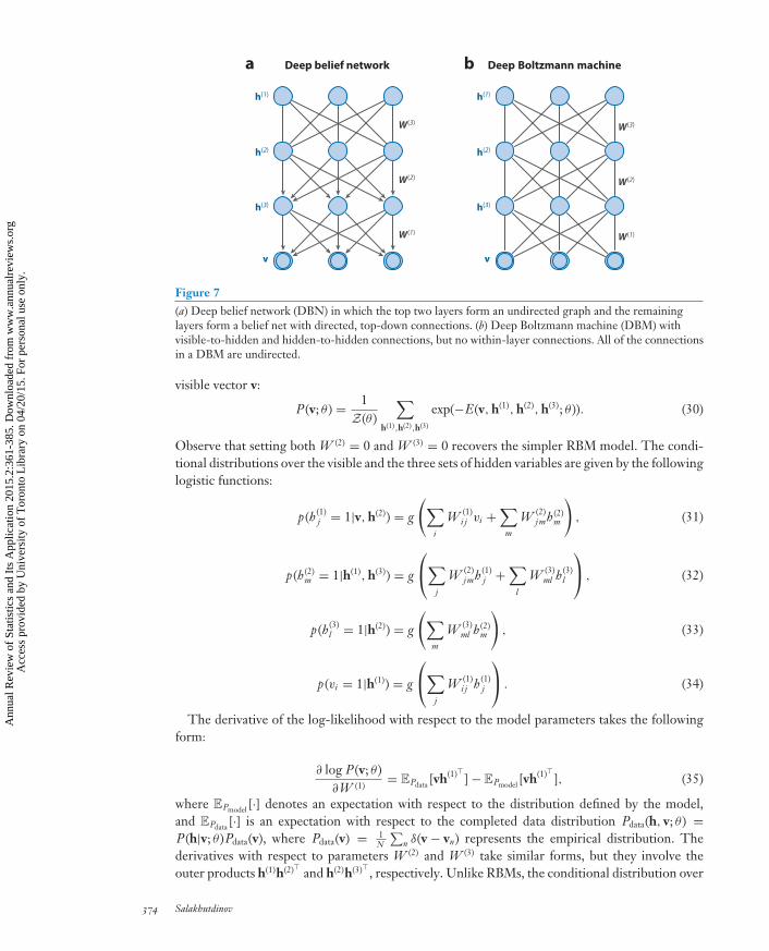
& Murray 2008). The estimates of the variational lower bound (see Equation 36) on the averagetest log-probability were −84.62 and −85.10 for the two- and three-layer DBMs, respectively.Observe that even though the two DBMs contain about 0.9 and 1.15 million parameters,respectively, they do not appear to suffer much from overfitting. The difference between theestimates of the training and test log-probabilities was approximately 1 nat. Figure 10 furthershows samples generated from the two models by randomly initializing all binary states andrunning the Gibbs sampler for 100,000 steps. All samples look like the real handwritten digits.

For a simple comparison, we also trained several mixture-of-Bernoullis models. We usedmodels with 10, 100, 500, 1000, and 2000 components. The corresponding average testlog-probabilities were −168.95, −142.63, −137.64, −133.21, and −135.78. Compared with aDBM, a mixture-of-Bernoullis model performs very poorly. The difference of about 50 nats pertest case is striking.

Training samples Two-layer DBM Three-layer DBM

Figure 10Random samples from the training set, and samples generated from two deep Boltzmann machines (DBMs)by running the Gibbs sampler for 100,000 steps. The images shown are the probabilities of the binary visiblevariables given the binary states of the hidden variables.

378 Salakhutdinov

Ann

ual R

evie

w o

f St

atis

tics

and

Its

App

licat

ion

2015

.2:3

61-3

85. D

ownl

oade

d fr

om w

ww

.ann

ualr

evie

ws.

org

Acc

ess

prov

ided

by

Uni

vers

ity o

f T

oron

to L

ibra

ry o

n 04

/20/

15. F

or p

erso

nal u

se o

nly.


Finally, after discriminative fine-tuning, the two-hidden-layer DBM achieves an error rateof 0.95% on the full MNIST test set.4 The three-layer DBM gives a slightly worse error rateof 1.01%. These DBM error rates are compared with error rates of 1.4%, achieved by supportvector machines (SVMs) (Decoste & Scholkopf 2002); 1.6%, achieved by a randomly initial-ized backpropagation algorithm; 1.2%, achieved by the DBN described in articles by Hinton &Salakhutdinov (2006) and Hinton et al. (2006); and 0.97%, obtained by using a combination ofdiscriminative and generative fine-tuning on the same DBN (Hinton 2007).

4.3.2. NORB data set. Results on the MNIST data set show that DBMs can significantly out-perform many other models on the well-studied but relatively simple task of handwritten digitrecognition. In this section we present results on the New York University Object RecognitionBenchmark (NORB) data set, which is a considerably more difficult data set than the MNISTdata set is. NORB (LeCun et al. 2004) contains images of 50 different three-dimensional (3D) toyobjects, with 10 objects in each of 5 generic classes (cars, trucks, planes, animals, and humans).Each object is photographed from different viewpoints and under various lighting conditions. Thetraining set contains 24,300 stereo image pairs of 25 objects, 5 per class, and the test set contains24,300 stereo pairs of the remaining different 25 objects. The goal is to classify each previouslyunseen object into its generic class.

We trained a two-hidden-layer DBM in which each layer contained 4,000 hidden variables,as shown in Figure 9b. Note that the entire model was trained in a completely unsupervisedway. After the subsequent discriminative fine-tuning, the “unrolled” DBM achieves a misclassi-fication error rate of 10.8% on the full test set. This error rate is compared with rates of 11.6%,achieved by SVMs (Bengio & LeCun 2007); 22.5%, achieved by logistic regression; and 18.4%,achieved by the k-nearest-neighbor approach (LeCun et al. 2004). To show that DBMs can benefitfrom additional unlabeled training data, we augmented the training data with additional unla-beled data by applying simple pixel translations, creating a total of 1,166,400 training instances.5

After learning a good generative model, the discriminative fine-tuning (using only the 24,300labeled training examples without any translation) reduces the misclassification error to 7.2%.Figure 11 shows samples generated from the model by running prolonged Gibbs sampling. Notethat the model was able to capture many regularities in this high-dimensional, richly structureddata, including variation in object classes, viewpoints, and lighting conditions.

Surprisingly, even though the DBM contains approximately 68 million parameters, it signifi-cantly outperforms many of the competing models. Clearly, unsupervised learning helps gener-alization because it ensures that most of the information in the model parameters comes frommodeling the input data. The very limited information in the labels is used only to slightly adjustthe layers of features already discovered by the DBM.

5. EXTENSIONS TO LEARNING FROM MULTIMODAL DATA

DBMs can be easily extended to modeling data that contain multiple modalities. The key ideais to learn a joint density model over the space of the multimodal inputs. For example, usinga large collection of user-tagged images, we can learn a joint distribution over images and text,P (vimg, vtxt; θ ) (Srivastava & Salakhutdinov 2014). By drawing samples from P (vtxt|vimg; θ ) and fromP (vimg, vtxt; θ ), we can fill in missing data, thereby doing image annotation [for P (vtxt|vimg; θ )] andimage retrieval [for P (vimg, vtxt; θ )].

4In the permutation-invariant version, the pixels of every image are subjected to the same random permutation, making ithard to use prior knowledge about images.5We thank Vinod Nair for sharing his code for blurring and translating NORB images.


Ann

ual R

evie

w o

f St

atis

tics

and

Its

App

licat

ion

2015

.2:3

61-3

85. D

ownl

oade

d fr

om w

ww

.ann

ualr

evie

ws.

org

Acc

ess

prov

ided

by

Uni

vers

ity o

f T

oron

to L

ibra

ry o

n 04

/20/

15. F

or p

erso

nal u

se o

nly.


Training samples Generated samples

Figure 11Random samples from the training set (left), and samples generated from a three-hidden-layer deepBoltzmann machine by running the Gibbs sampler for 10,000 steps (right).

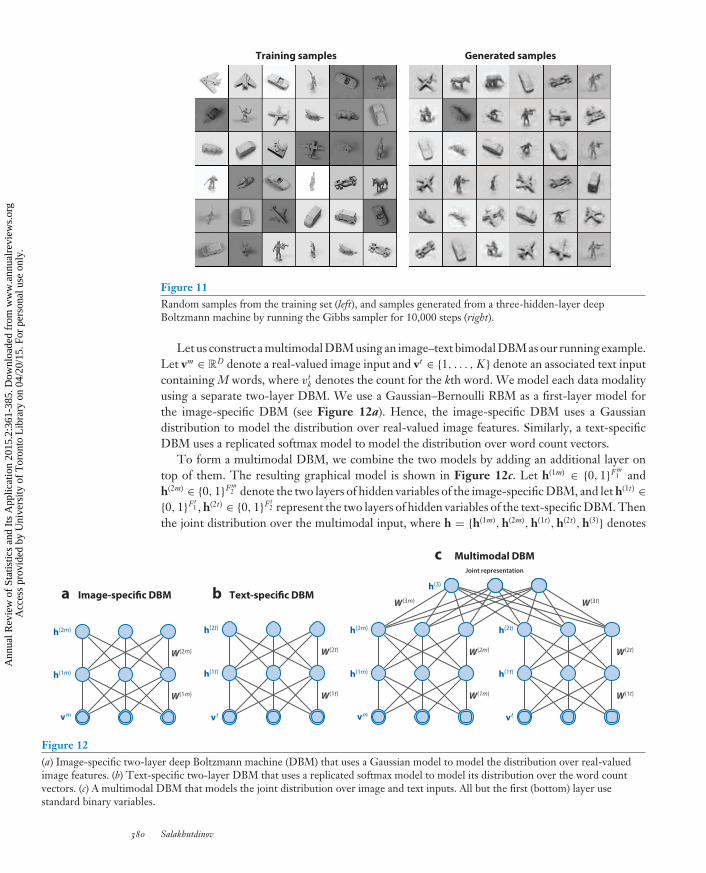
Let us construct a multimodal DBM using an image–text bimodal DBM as our running example.Let vm ∈ R

D denote a real-valued image input and vt ∈ {1, . . . , K } denote an associated text inputcontaining M words, where vt

k denotes the count for the kth word. We model each data modalityusing a separate two-layer DBM. We use a Gaussian–Bernoulli RBM as a first-layer model forthe image-specific DBM (see Figure 12a). Hence, the image-specific DBM uses a Gaussiandistribution to model the distribution over real-valued image features. Similarly, a text-specificDBM uses a replicated softmax model to model the distribution over word count vectors.

To form a multimodal DBM, we combine the two models by adding an additional layer ontop of them. The resulting graphical model is shown in Figure 12c. Let h(1m) ∈ {0, 1}Fm

1 andh(2m) ∈ {0, 1}Fm

2 denote the two layers of hidden variables of the image-specific DBM, and let h(1t) ∈{0, 1}Ft

1 , h(2t) ∈ {0, 1}Ft2 represent the two layers of hidden variables of the text-specific DBM. Then

the joint distribution over the multimodal input, where h = {h(1m), h(2m), h(1t), h(2t), h(3)} denotes

h(2m)

h(1m)

vm

W(2m)

W(1m)

h(2t)

h(1t)

vt

W(2t)

W(1t)

h(3)

h(2m)

h(1m)

vm

W(3m)

W(2m)

W(1m)

h(2t)

h(1t)

vt

W(3t)

W(2t)

W(1t)

Image-specific DBM Text-specific DBM

Multimodal DBMc

ba

Joint representation

Figure 12(a) Image-specific two-layer deep Boltzmann machine (DBM) that uses a Gaussian model to model the distribution over real-valuedimage features. (b) Text-specific two-layer DBM that uses a replicated softmax model to model its distribution over the word countvectors. (c) A multimodal DBM that models the joint distribution over image and text inputs. All but the first (bottom) layer usestandard binary variables.

380 Salakhutdinov

Ann

ual R

evie

w o

f St

atis

tics

and

Its

App

licat

ion

2015

.2:3

61-3

85. D

ownl

oade

d fr

om w

ww

.ann

ualr

evie

ws.

org

Acc

ess

prov

ided

by

Uni

vers

ity o

f T

oron

to L

ibra

ry o

n 04

/20/

15. F

or p

erso

nal u

se o

nly.


all hidden variables, is written as follows:

P (vm, vt ; θ ) =∑

h(2m),h(2t),h(3)

P (h(2m), h(2t), h(3))

⎛⎝∑

h(1m)

P (vm, h(1m)|h(2m))

⎞⎠

⎛⎝∑

h(1t)

P (vt, h(1t)|h(2t))

⎞⎠

= 1Z(θ, M )

∑h

exp

⎛⎝−

∑i

(vmi )2

2σ 2i

+∑

i j

vmi

σiW (1m)

i j h(1m)j +

∑j l

W (2m)j l h(1m)

j h(2m)l

︸︷︷︸Gaussian image pathway∑

kj

W (1t)kj vt

kh(1t)j +

∑j l

W (2t)j l h(1t)

j h(2t)l︸︷︷︸

Replicated softmax text pathway

+∑

l p

W (3t)h(2t)l h(3)

p +∑

l p

W (3m)h(2m)l h(3)

p +∑

p

b (3)p h(3)

p

⎞⎠

︸︷︷︸Joint third layer

.

(42)The normalizing constant depends on the number of words M in the corresponding documentbecause the low-level part of the text pathway contains as many softmax variables as there are wordsin the document. Similar to the replicated softmax model presented in Section 2.3, the multimodalDBM can be viewed as a family of different-sized DBMs that are created for documents of differentlengths that share parameters. Approximate learning and inference can proceed in the same wayas discussed in Section 4.1.

As an example, we now consider experimental results of using the MIR-Flickr data set (Huiskes& Lew 2008), which contains one million images retrieved from the social photography websiteFlickr, along with the user-assigned tags for these images. Bimodal data of this kind have becomecommon in many real-world applications in which we have some image and a few words describingit. There is a need to build representations that fuse this information into a joint space such thateach data point can be represented as a single vector. Such representation would be useful forclassification and retrieval problems.

Of 1 million images in the MIR-Flickr data set, 25,000 have been annotated using 38 classesincluding object categories such as “bird,” “tree,” and “people” and scene categories such as“indoor,” “sky,” and “night.” The remaining 975,000 images were unannotated. We used 10,000of the 25,000 annotated images for training, 5,000 for validation, and 10,000 for testing, followingthe experimental setup of Huiskes & Lew (2008).

In our multimodal DBM, the image pathway contained 3,857 linear visible variables6 and1,024 h(1) and 1,024 h(2) hidden variables. The text pathway consisted of a replicated softmax modelwith 2,000 visible variables and 1,024 hidden variables, followed by another layer of 1,024 hiddenvariables. The joint layer contained 2,048 hidden variables, and all hidden variables were binary.

Many real-world applications often have one or more modalities missing. The multimodalDBM can be used to generate such missing data modalities by clamping the observed modalities atthe inputs and sampling the hidden modalities by running a standard Gibbs sampler. For example,consider the generation of text conditioned on a given image7 vm. The observed modality vm

is clamped at the inputs, and all hidden variables are initialized randomly. Alternating Gibbssampling can be used to draw samples (or words) from P (vt |vm) by updating each hidden layergiven the states of the adjacent layers.8 This process is illustrated for a test image in Figure 13,

6Images were represented by 3,857-dimensional features, which were extracted by concatenating Pyramid Histogram ofWords (PHOW) features, Gist, and MPEG-7 descriptors (for details, see Srivastava & Salakhutdinov 2014).7Generation of image features conditioned on text can be done in a similar way.8Remember that the conditional distribution P (vt |h(1t)) defines a multinomial distribution over the text vocabulary (seeEquation 19). This distribution can then be used to sample words.


Ann

ual R

evie

w o

f St

atis

tics

and

Its

App

licat

ion

2015

.2:3

61-3

85. D

ownl

oade

d fr

om w

ww

.ann

ualr

evie

ws.

org

Acc

ess

prov

ided

by

Uni

vers

ity o

f T

oron

to L

ibra

ry o

n 04

/20/

15. F

or p

erso

nal u

se o

nly.


Step 50 Step 100 Step 150 Step 200 Step 250

travel beach sea water italytrip

vacationafrica

earthasiaasiamen2007india

tourism

ocean beach canada waterwaves island bc sea

sea vacation britishcolumbia boatsand travel reflection italianikon ocean alberta maresurf caribbean lake venizia

rocks tropical quebec acquacoast resort ontario oceanshore trip ice venice

Figure 13Text generated by the deep Boltzmann machine conditioned on an image by running a Gibbs sampler. Theten words with the highest probability are shown at the end of every 50 sampling steps.

which shows the text generated after every 50 Gibbs steps. Observe that the sampler generatesmeaningful text while showing some evidence of jumping across different modes. For example, itgenerates “tropical,” “caribbean,” and “resort” together, then moves on to “canada,” “bc,” “quebeclake,” “ice,” and then to “italia,” “venizia,” and “mare.” Each of these groups of words representplausible descriptions of the image. Moreover, each group is consistent within itself, suggestingthat that the model has been able to associate clusters of consistent descriptions with the sameimage. The model can also be used to generate images conditioned on text. Figure 14 showsexamples of two such runs.

The same DBM also achieves state-of-the-art classification results on the multimodal MIR-Flickr data set (Huiskes & Lew 2008), compared with linear discriminant analysis (LDA),RBF-kernel support vector machines (SVMs) (Huiskes & Lew 2008), and the multiple kernellearning approach of Guillaumin et al. (2010) (for details, see Srivastava & Salakhutdinov 2014).

6. CONCLUSIONS

This article has reviewed several deep generative models, including DBNs and DBMs. We showedthat learning deep generative models that contain many layers of latent variables and millionsof parameters can be carried out efficiently. Learned high-level feature representations can be

Input tags

purple,flowers

car,automobile

Step 50 Step 100 Step 150 Step 200 Step 250

Figure 14Images retrieved by running a Gibbs sampler conditioned on the input tags “purple,” “flowers” (top row) and“car,” “automobile” (bottom row). The images shown are those which are closest to the sampled imagefeatures. Samples were taken after every 50 steps.

382 Salakhutdinov

Ann

ual R

evie

w o

f St

atis

tics

and

Its

App

licat

ion

2015

.2:3

61-3

85. D

ownl

oade

d fr

om w

ww

.ann

ualr

evie

ws.

org

Acc

ess

prov

ided

by

Uni

vers

ity o

f T

oron

to L

ibra

ry o

n 04

/20/

15. F

or p

erso

nal u

se o

nly.


successfully applied in a wide spectrum of application domains, including visual object recognition,information retrieval, classification tasks, and regression tasks. Many of the ideas developed in thisarticle are based on the following three crucial principles behind learning deep generative models:First, multiple layers of representation can be greedily learned one layer at a time. Second, greedylearning can be carried out in a completely unsupervised way. Third, a separate fine-tuning stagecan be used to further improve either generative or discriminative performance of the final model.Furthermore, using stochastic gradient descent, scaling up learning to billions of data points wouldnot be particularly difficult.

We also developed a new learning algorithm for DBMs. Similar to DBNs, DBMs contain manylayers of latent variables. High-level representations are built from large amounts of unlabeledsensory input, and the limited labeled data can then be used to slightly adjust the model parametersfor a specific task at hand. We discussed a novel combination of variational and MCMC algorithmsfor training these Boltzmann machines. When applied to DBMs with several hidden layers andmillions of weights, this combination is a very effective way to learn good generative models. Wedemonstrated the performance of this algorithm using both the MNIST data set of handwrittendigits and the NORB data set of stereo images of 3D objects with highly variable viewpoints andlighting.

Finally, we discussed a DBM model for learning multimodal data representations. Largeamounts of unlabeled data can be effectively utilized by the model, in which pathways for eachdifferent modality are pretrained independently and later combined together for performing jointlearning. The model fuses multiple data modalities into a unified representation, capturing fea-tures that are useful for classification and retrieval. Indeed, this model was able to discover a diverseset of plausible descriptions given a test image and to achieve state-of-the-art classification resultson the bimodal MIR-Flickr data set.

DISCLOSURE STATEMENT

The author is not aware of any affiliations, memberships, funding, or financial holdings that mightbe perceived as affecting the objectivity of this review.

ACKNOWLEDGMENTS

This research was supported by CIFAR, Google, Samsung, and ONR Grant N00014-14-1-0232.

LITERATURE CITED

Bengio Y. 2009. Learning deep architectures for AI. Found. Trends Mach. Learn. 2:1–127Bengio Y, Lamblin P, Popovici D, Larochelle H. 2007. Greedy layer-wise training of deep networks. Adv.

Neural Inf. Process. Syst. 19:153–60Bengio Y, LeCun Y. 2007. Scaling learning algorithms towards AI. In Large-Scale Kernel Machines, ed. L

Bottou, O Chapelle, D DeCoste, J Weston, pp. 321–360. Cambridge, MA: MIT PressBlei DM, Ng AY, Jordan MI. 2003. Latent Dirichlet allocation. J. Mach. Learn. Res. 3:993–1022Blei DM. 2014. Build, compute, critique, repeat: data analysis with latent variable models. Annu. Rev. Stat.

Appl. 1:203–32Collobert R, Weston J. 2008. A unified architecture for natural language processing: deep neural networks

with multitask learning. Proc. 25th Int. Conf. Mach. Learn. Helsinki, Jul. 5–9, pp. 160–67. New York: ACMDahl GE, Jaitly N, Salakhutdinov R. 2014. Multi-task neural networks for QSAR predictions. arXiv:1406.1231

[stat.ML]Decoste D, Scholkopf B. 2002. Training invariant support vector machines. Mach. Learn. 46:161–90


Ann

ual R

evie

w o

f St

atis

tics

and

Its

App

licat

ion

2015

.2:3

61-3

85. D

ownl

oade

d fr

om w

ww

.ann

ualr

evie

ws.

org

Acc

ess

prov

ided

by

Uni

vers

ity o

f T

oron

to L

ibra

ry o

n 04

/20/

15. F

or p

erso

nal u

se o

nly.


Guillaumin M, Verbeek J, Schmid C. 2010. Multimodal semi-supervised learning for image classification. Proc.IEEE Conf. Comput. Vis. Pattern Recognit., San Francisco, Jun. 13–18, pp. 902–9. Piscataway, NJ: IEEE

Hinton GE. 2002. Training products of experts by minimizing contrastive divergence. Neural Comput.14(8):1711–800

Hinton GE. 2007. To recognize shapes, first learn to generate images. Prog. Brain Res. 165:535–47Hinton GE, Salakhutdinov RR. 2006. Reducing the dimensionality of data with neural networks. Science

313(5786):504–7Hinton GE, Sejnowski T. 1983. Optimal perceptual inference. Proc. IEEE Conf. Comput. Vis. Pattern Recognit.,

Washington, DC, pp. 448–53. Silver Spring, MD: IEEEHinton GE, Osindero S, Teh Y-W. 2006. A fast learning algorithm for deep belief nets. Neural Comput.

18(7):1527–54Hinton G, Deng L, Yu D, Dahl GE, Mohamed A, et al. 2012. Deep neural networks for acoustic modeling

in speech recognition: the shared views of four research groups. IEEE Signal Process. Mag. 29(6):82–97Hofmann T. 1999. Probabilistic latent semantic analysis. Proc. 15th Conf. Uncertainty in Artif. Intell., Stockholm,

Swe., Jul. 30–Aug. 1, pp. 289–96. San Francisco: Morgan KaufmannHuiskes MJ, Lew MS. 2008. The MIR Flickr retrieval evaluation. Proc. 16th Int. Conf. Multimed. Inf. Retr.,

Vancouver, Can., Oct. 30–31. New York: ACMKrizhevsky A, Sutskever I, Hinton GE. 2012. ImageNet classification with deep convolutional neural networks.

Adv. Neural Inf. Process. Syst. 25:1106–14Larochelle H, Bengio Y, Louradour J, Lamblin P. 2009. Exploring strategies for training deep neural networks.

J. Mach. Learn. Res. 10:1–40LeCun Y, Huang FJ, Bottou L. 2004. Learning methods for generic object recognition with invariance to

pose and lighting. Proc. IEEE Conf. Comput. Vis. Pattern Recognit., Washington, DC, Jun. 27–Jul. 2, vol. 2,pp. 97–104. Los Alamitos, CA: IEEE

Lee H, Grosse R, Ranganath R, Ng AY. 2009. Convolutional deep belief networks for scalable unsupervisedlearning of hierarchical representations. Proc. 26th Intl. Conf. Mach. Learn. Montreal, Jun. 14–18, pp. 609–16. New York: ACM

Lee TS, Mumford D, Romero R, Lamme V. 1998. The role of the primary visual cortex in higher level vision.Vision Res. 38:2429–54

Lenz I, Lee H, Saxena A. 2013. Deep learning for detecting robotic grasps. Proc. Robot. Sci. Syst. IX Berlin,Ger., Jun. 24–28. http://www.roboticsproceedings.org/rss09/p12.pdf

Memisevic R, Hinton GE. 2010. Learning to represent spatial transformations with factored higher-orderBoltzmann machines. Neural Comput. 22(6):1473–92

Mohamed A, Dahl GE, Hinton G. 2012. Acoustic modeling using deep belief networks. IEEE Trans. AudioSpeech Lang. Proc. 20:14–22

Nair V, Hinton GE. 2009. Implicit mixtures of restricted Boltzmann machines. Adv. Neural Inf. Process. Syst.21:1145–52

Neal RM. 2001. Annealed importance sampling. Stat. Comput. 11:125–39Ranzato MA, Huang F, Boureau Y, LeCun Y. 2007. Unsupervised learning of invariant feature hierarchies

with applications to object recognition. Proc. IEEE Conf. Comput. Vis. Pattern Recognit., Minneapolis, MN,June 18–23, pp. 1–8. Piscataway, NJ: IEEE. doi: 10.1109/CVPR.2007.383157

Ranzato M, Boureau Y-L, LeCun Y. 2008. Sparse feature learning for deep belief networks. Adv. NeuralInform. Proc. Syst. 20:1185–92

Robbins H, Monro S. 1951. A stochastic approximation method. Ann. Math. Stat. 22:400–7Rumelhart DE, Hinton GE, Williams RJ. 1986. Learning representations by back-propagating errors. Nature

323:533–36Salakhutdinov RR. 2008. Learning and evaluating Boltzmann machines. Tech. Rep. UTML TR 2008-002, Dep.

Comput. Sci., Univ. Toronto, TorontoSalakhutdinov RR, Hinton GE. 2007. Learning a nonlinear embedding by preserving class neighbourhood

structure. Proc. 11th Int. Conf. Artif. Intell. Stat., San Juan, PR, Mar. 21–24, pp. 412–19. Brookline, MA:Microtome

Salakhutdinov RR, Hinton GE. 2008. Using deep belief nets to learn covariance kernels for Gaussian processes.Adv. Neural Inf. Process. Syst. 20:1249–56

384 Salakhutdinov

Ann

ual R

evie

w o

f St

atis

tics

and

Its

App

licat

ion

2015

.2:3

61-3

85. D

ownl

oade

d fr

om w

ww

.ann

ualr

evie

ws.

org

Acc

ess

prov

ided

by

Uni

vers

ity o

f T

oron

to L

ibra

ry o

n 04

/20/

15. F

or p

erso

nal u

se o

nly.

http://www.roboticsproceedings.org/rss09/p12.pdf


Salakhutdinov RR, Hinton GE. 2009a. Deep Boltzmann machines. Proc. 12th Int. Conf. Artif. Intell. Stat.,Clearwater Beach, FL, Apr. 16–18, pp. 448–55. Brookline, MA: Microtome

Salakhutdinov RR, Hinton GE. 2009b. Replicated softmax: an undirected topic model. Adv. Neural Inf. Proc.Syst. 22:1607–14

Salakhutdinov RR, Hinton GE. 2009c. Semantic hashing. Int. J. Approx. Reason.50:969–78Salakhutdinov RR, Hinton GE. 2013. Modeling documents with Deep Boltzmann Machines. Proc. 29th Conf.

Uncertain. Artif. Intell., Bellevue, WA, Jul. 11–15, pp. 616–24. Corvallis, OR: AUAI PressSalakhutdinov RR, Murray I. 2008. On the quantitative analysis of deep belief networks. Proc. 25th Int. Conf.

Mach. Learn., Helsinki, Jul. 5–9, pp. 872–79. New York: ACMSerre T, Oliva A, Poggio TA. 2007. A feedforward architecture accounts for rapid categorization. PNAS

104:6424–29Smolensky P. 1986. Information processing in dynamical systems: foundations of harmony theory. In Parallel

Distributed Processing, ed. DE Rumelhart, JL McClelland, chapter 6, pp. 194–281. Cambridge, MA: MITPress

Socher R, Huang EH, Pennington J, Ng AY, Manning CD. 2011. Dynamic pooling and unfolding recursiveautoencoders for paraphrase detection. Adv. Neural Inf. Process. Syst. 24:801–9

Srivastava N, Salakhutdinov R. 2014. Multimodal learning with deep Boltzmann machines. J. Machine Learn.Res. 15:2949–80

Sutskever I, Martens J, Dahl G, Hinton G. 2013. On the importance of momentum and initialization in deeplearning. Proc. 30th Int. Conf. Mach. Learn., Atlanta, Jun. 16–21, pp. 1139–47

Taylor G, Hinton GE, Roweis ST. 2006. Modeling human motion using binary latent variables. Adv. NeuralInf. Process. Syst. 19:1345–52

Taylor GW, Fergus R, LeCun Y, Bregler C. 2010. Convolutional learning of spatio-temporal features. Proc.11th Eur. Conf. Comput. Vis., Crete, Greece, Sep. 5–11, pp. 140–153. Berlin: Springer

Tieleman T. 2008. Training restricted Boltzmann machines using approximations to the likelihood gradient.Proc. 25th Int. Conf. Mach. Learn., Helsinki, Jul. 5–9, pp. 1064–71. New York: ACM

Torralba A, Fergus R, Weiss Y. 2008. Small codes and large image databases for recognition. Proc. IEEEConf. Comput. Vis. Pattern Recognit. Anchorage, AK, Jun. 23–28, pp. 1–8. Silver Spring, MD: IEEE. doi:10.1109/CVPR.2008.4587633

Uria B, Murray I, Larochelle H. 2014. A deep and tractable density estimator. Proc. 31st Int. Conf. Mach.Learn., Beijing, Jun. 21–26, pp. 467–75. Brookline, MA: Microtome

Vincent P, Larochelle H, Bengio Y, Manzagol P. 2008. Extracting and composing robust features with de-noising autoencoders. Proc. 25th Int. Conf. Mach. Learn., Helsinki, Jul. 5–9, pp. 1096–103. New York:ACM

Wang T, Wu D, Coates A, Ng AY. 2012. End-to-end text recognition with convolutional neural networks.Proc. 21st Int. Conf. Pattern Recognit., Tsukuba, Jpn., Nov. 11–15, pp. 3304–8. Piscataway, NJ: IEEE

Welling M, Rosen-Zvi M, Hinton GE. 2005. Exponential family harmoniums with an application to infor-mation retrieval. Adv. Neural Inf. Process. Syst. 17:1481–88

Younes L. 1989. Parameter inference for imperfectly observed Gibbsian fields. Probab. Theory Rel. Fields82:625–45

Younes L. 1999. On the convergence of Markovian stochastic algorithms with rapidly decreasing ergodicityrates. Stoch. Stoch. Rep. 65:177–228

Yuille AL. 2004. The convergence of Contrastive Divergences. Adv. Neural Inf. Process. Syst. 17:1593–600


Ann

ual R

evie

w o

f St

atis

tics

and

Its

App

licat

ion

2015

.2:3

61-3

85. D

ownl

oade

d fr

om w

ww

.ann

ualr

evie

ws.

org

Acc

ess

prov

ided

by

Uni

vers

ity o

f T

oron

to L

ibra

ry o

n 04

/20/

15. F

or p

erso

nal u

se o

nly.

ST02-FrontMatter ARI 25 March 2015 8:0

Annual Review ofStatistics and ItsApplication

Volume 2, 2015ContentsReproducing Statistical Results

Victoria Stodden � � � � � � � � � � � � � � � � � � � � � � � � � � � � � � � � � � � � � � � � � � � � � � � � � � � � � � � � � � � � � � � � � � � � � � � � � � � � � � � � 1

How to See More in Observational Studies: Some NewQuasi-Experimental DevicesPaul R. Rosenbaum � � � � � � � � � � � � � � � � � � � � � � � � � � � � � � � � � � � � � � � � � � � � � � � � � � � � � � � � � � � � � � � � � � � � � � � � � � � �21

Incorporating Both Randomized and Observational Data into aSingle AnalysisEloise E. Kaizar � � � � � � � � � � � � � � � � � � � � � � � � � � � � � � � � � � � � � � � � � � � � � � � � � � � � � � � � � � � � � � � � � � � � � � � � � � � � � � �49

Microbiome, Metagenomics, and High-Dimensional CompositionalData AnalysisHongzhe Li � � � � � � � � � � � � � � � � � � � � � � � � � � � � � � � � � � � � � � � � � � � � � � � � � � � � � � � � � � � � � � � � � � � � � � � � � � � � � � � � � � � �73

Multiset Statistics for Gene Set AnalysisMichael A. Newton and Zhishi Wang � � � � � � � � � � � � � � � � � � � � � � � � � � � � � � � � � � � � � � � � � � � � � � � � � � � � � � �95

Probabilistic Record Linkage in Astronomy: DirectionalCross-Identification and BeyondTamas Budavari and Thomas J. Loredo � � � � � � � � � � � � � � � � � � � � � � � � � � � � � � � � � � � � � � � � � � � � � � � � � � � 113

A Framework for Statistical Inference in AstrophysicsChad M. Schafer � � � � � � � � � � � � � � � � � � � � � � � � � � � � � � � � � � � � � � � � � � � � � � � � � � � � � � � � � � � � � � � � � � � � � � � � � � � � 141

Modern Statistical Challenges in High-Resolution FluorescenceMicroscopyTimo Aspelmeier, Alexander Egner, and Axel Munk � � � � � � � � � � � � � � � � � � � � � � � � � � � � � � � � � � � � � 163

Statistics of ExtremesA.C. Davison and R. Huser � � � � � � � � � � � � � � � � � � � � � � � � � � � � � � � � � � � � � � � � � � � � � � � � � � � � � � � � � � � � � � � � � 203

Multivariate Order Statistics: Theory and ApplicationGrant B. Weller and William F. Eddy � � � � � � � � � � � � � � � � � � � � � � � � � � � � � � � � � � � � � � � � � � � � � � � � � � � � 237

Agent-Based Models and MicrosimulationDaniel Heard, Gelonia Dent, Tracy Schifeling, and David Banks � � � � � � � � � � � � � � � � � � � � � � � 259

Statistical Causality from a Decision-Theoretic PerspectiveA. Philip Dawid � � � � � � � � � � � � � � � � � � � � � � � � � � � � � � � � � � � � � � � � � � � � � � � � � � � � � � � � � � � � � � � � � � � � � � � � � � � � � 273

vii

Ann

ual R

evie

w o

f St

atis

tics

and

Its

App

licat

ion

2015

.2:3

61-3

85. D

ownl

oade

d fr

om w

ww

.ann

ualr

evie

ws.

org

Acc

ess

prov

ided

by

Uni

vers

ity o

f T

oron

to L

ibra

ry o

n 04

/20/

15. F

or p

erso

nal u

se o

nly.

ST02-FrontMatter ARI 25 March 2015 8:0

Using Longitudinal Complex Survey DataMary E. Thompson � � � � � � � � � � � � � � � � � � � � � � � � � � � � � � � � � � � � � � � � � � � � � � � � � � � � � � � � � � � � � � � � � � � � � � � � � � 305

Functional RegressionJeffrey S. Morris � � � � � � � � � � � � � � � � � � � � � � � � � � � � � � � � � � � � � � � � � � � � � � � � � � � � � � � � � � � � � � � � � � � � � � � � � � � � � 321

Learning Deep Generative ModelsRuslan Salakhutdinov � � � � � � � � � � � � � � � � � � � � � � � � � � � � � � � � � � � � � � � � � � � � � � � � � � � � � � � � � � � � � � � � � � � � � � � 361

viii Contents

Ann

ual R

evie

w o

f St

atis

tics

and

Its

App

licat

ion

2015

.2:3

61-3

85. D

ownl

oade

d fr

om w

ww

.ann

ualr

evie

ws.

org

Acc

ess

prov

ided

by

Uni

vers

ity o

f T

oron

to L

ibra

ry o

n 04

/20/

15. F

or p

erso

nal u

se o

nly.

Documents

Learning Deep Generative Models - Carnegie Mellon …rsalakhu/papers/annrev.pdf · Recently, Hinton et al. (2006) introduced a moderately fast, unsupervised learning algorithm for