Embed Size (px)
Citation preview
DAP Report
Learning Deep Generative Models
With Discrete Latent Variables
Hengyuan HuDepartment of Machine Learning
Carnegie Mellon [email protected]
28 Nov 2017
Abstract
There have been numerous recent advancements on learning deep generative models with latentvariables thanks to the reparameterization trick that allows to train deep directed models effectively.However, since reparameterization trick only works on continuous variables, deep generative modelswith discrete latent variables still remain hard to train and perform considerably worse than theircontinuous counterparts. In this paper, we attempt to shrink this gap by introducing a newarchitecture and its learning procedure. We develop a hybrid generative model with binary latentvariables that consists of an undirected graphical model and a deep neural network. We proposean efficient two-stage pretraining and training procedure that is crucial for learning these models.Experiments on binarized digits and images of natural scenes demonstrate that our model achievesclose to the state-of-the-art performance in terms of density estimation and is capable of generatingcoherent images of natural scenes.
DAP Committee members:
Ruslan Salakhutdinov 〈 [email protected] 〉 (Advisor)Aarti Singh 〈 [email protected] 〉Barnabas Poczos 〈 [email protected] 〉
1 of 19
DAP Report
1 Introduction
Building generative models that are capable of learning flexible distributions over high-dimensionalsensory input, such as images of natural scenes, is one of the fundamental problems in unsupervisedlearning. Historically, many multi-layer generative models, including sigmoid belief networks(SBNs) [1], deep belief networks (DBNs) [2], and deep Boltzmann machines (DBMs) [3], containmultiple layers of binary stochastic variables. However, since the debut of variational autoencoder(VAE) [4] and reparameterization trick, models with continuous variables have largely replacedprevious discrete versions. Many improvements [5; 6; 7; 8] along this direction have been pushingforward the state-of-the-art for years.
Comparing with continuous models, existing discrete models have two major disadvantages. First,models with continuous latent variables are easier to optimize due to the reparameterization trick.Second, every layer in models, including SBNs and DBNs, is stochastic. Such design pattern restrictsthe depth of these models because adding one layer can only provide small additional representationpower while the extra stochasticity increases the optimization difficulty and thus out-weights thebenefit.
In this paper we explore learning discrete latent variable models that perform equally well with itscontinuous counterparts. Specifically, we propose an architecture that resembles the DBN but usesdeep deterministic neural networks for inference and generative networks. From the VAE perspective,this can also be seen as deep VAE with one set of binary latent variables and learnable restrictedBoltzmann machine (RBM) prior [9]. We develop a two-stage pretraining, training procedure forlearning such models and show that they are necessary and effective. Finally, we demonstratethat our models can closely match the state-of-the-art continuous models on MNIST in terms oflog-likelihood and are capable of generating coherent images of natural scenes.
2 Background
Although discrete models are largely replaced by continuous models in practice, there has been asurge in the interest of the learning algorithms that accommodate discrete latent variable models,such as sigmoid belief networks (SBNs) [10; 11; 12]. In this section, we briefly review those methodsthat lay the foundation of our learning procedure.
To learn a generative model p(x) on a given dataset, we introduce latent variable z and decomposethe objective as log p(x) = log
∑z p(x, z). Posteriors samples from p(z|x) are required to efficiently
estimate the exponential sum∑
z p(x, z). However, when p(x, z) is parameterized by a deep neuralnetwork, exact posterior sampling is no longer possible. One way to overcome it is to simultaneouslytrain an inference network q(z|x) that approximates the true posterior p(z|x). With samples from q
2 of 19
DAP Report
distribution, we can train p by optimizing the variational lower bound:
log p(x) = log
[∑z
p(x|z)p(z)
q(z|x)q(z|x)
]≥ Ez∼q(z|x) log
p(x, z)
q(z|x)(1)
Meanwhile, q(z|x) has to be optimized towards p(z|x) in order to keep the variational bound tight.
In the Wake-Sleep algorithm [13; 2], the wake phase corresponds to maximizing the objective inEq. 1 with respect to the parameter of p(x, z) using samples from q(z|x) given a datapoint x. Inthe sleep phase, a pair of samples z,x is drawn from the generative distribution p(x, z) and thenq is trained to minimize the KL divergence KL(p(z|x) ‖ q(z|x)). This objective, however, is nottheoretically sound as we should instead be minimizing its reverse: KL(q(z|x) ‖ p(z|x)).
Reweighted Wake-Sleep (RWS) [11] brings two major improvements to the original Wake-Sleepalgorithm. The first one is to reformulate the log-likelihood objective as an importance-weightedaverage and derive a tighter lower bound:
log p(x) = logEzi∼q(z|x)
[1
K
K∑i=1
p(x, zi)
q(zi|x)
]≥ Ezi∼q(z|x)
[log
1
K
K∑i=1
p(x, zi)
q(zi|x)
]= LK . (2)
In the wake phase of RWS, parameters in p are learned by optimizing the new lower bound definedin Eq. 2 [5]. The second improvement is to add a wake phase for learning q. The wake phase for qcan be viewed as minimizing the KL divergence KL(p(z|x) ‖ q(z|x)) for a given datapoint xdata
instead of xsample as in the sleep phase. The authors empirically show that the new wake phaseworks better than the sleep phase in the original Wake-Sleep and works even better when combinedwith the sleep phase.
Although RWS tightens the bound and works well in practice, it still does not optimize a well-definedobjective for inference network q. [12] propose a new method named VIMCO, which solves thisproblem. In VIMCO, both p and q are optimized jointly against the lower bound in Eq. 2. However,the gradient w.r.t parameters in q will have high variance if we compute them naively. VIMCOalgorithm utilizes the multiple samples to compose a baseline for each sample using the rest ofsamples (we refer readers to the original paper for more technical details). The author shows thatVIMCO performs equally well as RWS when training SBNs on MNIST.
3 Model
Let us consider a latent variable model p(x) =∑
z p(x|z)p(z) with the distribution p(z) defined overthe latent space. In addition, an inference network q(z|x) is used to approximate the intractableposterior distribution p(z|x). This fundamental formulation is shared by many deep generativemodels with latent variables, including deep belief networks (DBNs), and variational autoencoders
3 of 19
DAP Report
(VAEs). Different realizations result in different architectures and corresponding learning algorithms.In our model, the prior distribution pϕ(z) is multivariate Bernoulli modeled by a restricted Boltzmannmachine (RBM) with a parameter vector ϕ. The approximate posterior distribution qφ(z|x) ismultivariate Bernoulli with its mean modeled by a deep neural network φ. The generative distributionpθ(x|z) is modeled by a deep neural network θ as well. Note that both networks are deterministic.
This model has several advantages. First, compared with VAEs, RBMs can handle both discrete andcontinuous latent variables. It also allows for a much richer family of latent distributions comparedto simple factorized distributions as in vanilla VAEs. Although for VAEs, the posterior distributionis regularized towards a factorized Gaussian prior by minimizing KL divergence, in practice the KLdivergence is never zero, especially when modeling complex datasets. Such discrepancy between theprior and learned posterior can often damage the generative quality. The RBM approach, however,instead of pulling the posterior to some pre-defined prior, learns to mimic the posterior. Duringgeneration process, prior samples drawn by running the Markov chain defined by the RBM canoften lead to images with higher visual quality than those drawn from vanilla VAEs.
Second, compared with SBNs and DBNs, only communication between inference and generativenetworks uses stochastic binary states. In this case, the inference and generative networks becomefully differentiable so that multiple layers can be jointly optimized by back-propagation. Thisis radically different from SBNs and DBNs where each inference layer is trained to approximatethe posterior distribution of a specific generative layer. Our framework can greatly increase themodel capacity by allowing more complicated transformation between high dimensional input spaceand latent space. In addition, networks can exploit modern network design techniques, includingconvolution, pooling, dropout [14], or even ResNet [15] and DenseNet [16], in a very easy andstraightforward way. Therefore, similar to VAEs, models under this framework can be scaled tohandle more complex datasets compared to traditional SBNs and DBNs.
3.1 Pretraining with Autoencoder
Training a hybrid model is never a trivial task. Notably in our case, the encoder and decodernetworks can be very deep and gradient cannot be propagated through stochastic states. In addition,RBMs are often more sensitive to training compared to feed-forward neural networks. Therefore, asin DBNs and DBMs, a clever pretraining algorithm that can help find a good weight initializationcan be very beneficial.
To learn a good image prior, we jointly train parameters of the inference network φ and generativenetwork θ as an autoencoder. To obtain a binary latent space, we use additive i.i.d uniform noise [17]together with a modified hardtanh function to realize “soft-binarization”. This method can be
4 of 19

DAP Report
described as the following function:
B(z) = f(z + U(−0.5, 0.5)), where f(x) =
0, x ≤ 0
x, 0 ≤ x ≤ 1
1, x ≥ 1
(3)
and z = E(x) is the output of the encoder. This soft-binarization function will encourage theencoder to encode x into ([−∞,−1] ∪ [1,+∞])|z| to maximize the information that follows throughthis bottleneck while allowing gradient descent methods to find such solution efficiently. To avoidoverfitting, dropout can be applied after B function. The adoption of dropout in z space can alsoprevent the co-adaptation between latent codes, which makes it easier for RBMs to model.
In practice, we find that this pretraining procedure produces well binarized latent space on whichRBMs can be successfully trained. Therefore, we can then pretrain the RBMs on z using contrastivedivergence [9] or persistent contrastive divergence [18]. After pretraining, we remove B and appenda sigmoid function σ to the end of the encoder to convert it to the inference network, i.e.φ = σ ◦ E .The decoder is then used to initialize the generator θ.
3.2 Training
Since our model shares the fundamental formulation with many of the existing variational basedmodels, we can modify the state-of-the-art learning algorithms to train it. The specific algorithmswe are interested in are the reweighted wake-sleep (RWS) [11] and VIMCO [12] which give the bestresults on SBN models and can handle discrete latent variables.
As reviewed in the background section, both RWS and VIMCO are importance sampling basedmethods, that need to compute weights wi = p(x, zi)/q(x|zi) for multiple samples zi given input x.These weights are then normalized as wi = wi/(
∑j wj) to decide the contribution of each sample to
the gradient estimator. In our model, the joint probability p(x, z) is intractable due to the partitionZ function introduced by RBM. However, it can be substituted by its unnormalized counterpart:
p∗(x, z) = Zp(x, z) = e−F(z)p(x|z), (4)
as the coefficient Z will be canceled during the weight normalization step. The F(z) is the freeenergy assigned to z by RBM, which can be computed analytically.
The RBM is also trained using multiple samples as part of the generative module. In both RWSand VIMCO, the gradient for RBM with parameter ϕ is:
∂
∂ϕLK '
K∑i=1
wi∂
∂ϕlog pϕ(zi) = −
K∑i=1
wi∂F(zi)
∂ϕ+ Ez−∼M
[∂F(z−)
∂ϕ
]. (5)
5 of 19
DAP Report
The second term in Eq. 5 is the intractable model dependent term which needs to be estimatedusing samples from the RBM. The samples are obtained by running a persistent Markov chain as inpersistent contrastive divergence [18].
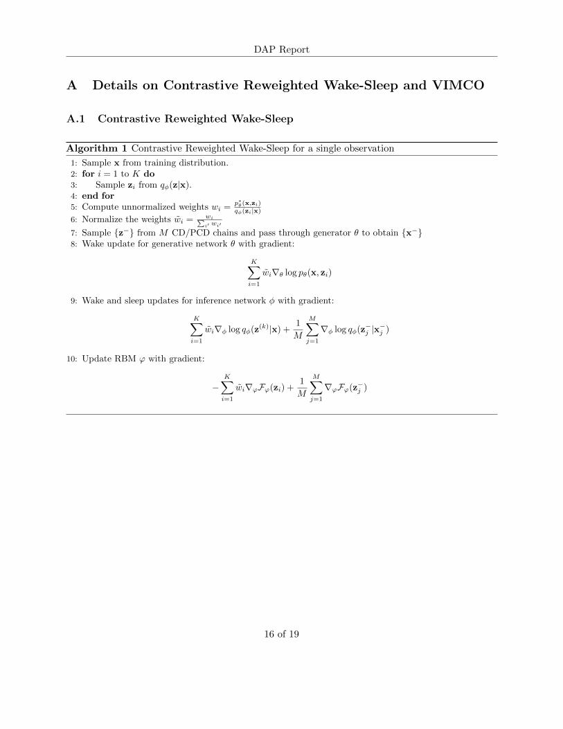
There is one more modification for the sleep phase in RWS. The generative process now starts froma Markov chain defined by RBM instead of a direct draw from unconditional Bernoulli prior. Thiscan be seen as the contrastive version of RWS. For completeness, we put the detail of ContrastiveRWS and VIMCO in Appendix A.
3.3 Evaluation
Quantitative evaluation of deep generative models is very crucial to measure and compare differentprobabilistic models. Fortunately, we can refer to a rich set of existing techniques for quantitativeevaluations. One way to evaluate our model is to decompose the lower bound LK in Eq. 1 as follows:
LK = Ezi∼q(z|x)
[log
1
K
K∑i=1
p∗(x, zi)
q(zi|x)
]− logZ (6)
and estimate partition function Z with Annealed Importance Sampling (AIS) [19]. This methodis very efficient since we only need to estimate Z once no matter how large the K is. However,since AIS gives an unbiased estimate of Z, it on average tends to underestimate logZ sincelogZ = logE(Z) ≥ E(log Z) [20].
Another method that yields conservative estimates is Reverse AIS Estimator (RAISE) [20], whichreturns an unbiased estimate of p(z). However, RAISE can be quite time consuming since it needs torun an independent chain for every z. Therefore, we suggest to use AIS as main tool for evaluationduring training and model comparison, since empirically AIS provides fairly accurate estimates,but also run RAISE as a safety check before reporting final results to avoid unrealistically highestimates of LK .
4 Related Work
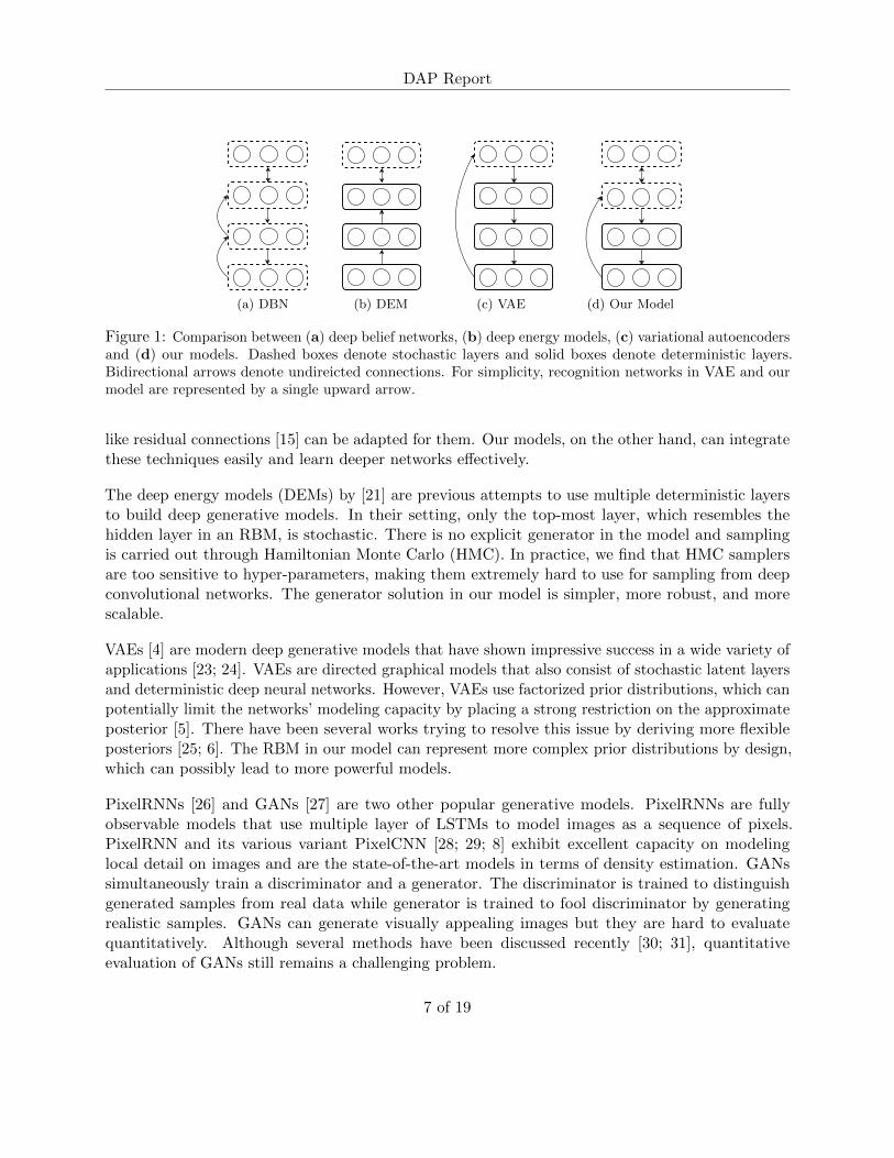
In Figure 1, we show the visualization of our model together with three closely related existinglatent variable models, DBNs [2], DEMs [21] and VAEs [4].
The major difference between DBNs and our models is that every layer in the inference and generativenetworks in DBNs is stochastic. Such design drastically increases the difficulty in training andrestrict the model from using modern deep convolutional architectures. Although convolution,combined with a sophisticated probabilistic pooling technique, has been applied to DBNs [22], theresulted convolutional DBNs is still difficult to train. It is also unclear how more recent techniques
6 of 19
DAP Report
(a) DBN (b) DEM (c) VAE (d) Our Model
Figure 1: Comparison between (a) deep belief networks, (b) deep energy models, (c) variational autoencodersand (d) our models. Dashed boxes denote stochastic layers and solid boxes denote deterministic layers.Bidirectional arrows denote undireicted connections. For simplicity, recognition networks in VAE and ourmodel are represented by a single upward arrow.
like residual connections [15] can be adapted for them. Our models, on the other hand, can integratethese techniques easily and learn deeper networks effectively.
The deep energy models (DEMs) by [21] are previous attempts to use multiple deterministic layersto build deep generative models. In their setting, only the top-most layer, which resembles thehidden layer in an RBM, is stochastic. There is no explicit generator in the model and samplingis carried out through Hamiltonian Monte Carlo (HMC). In practice, we find that HMC samplersare too sensitive to hyper-parameters, making them extremely hard to use for sampling from deepconvolutional networks. The generator solution in our model is simpler, more robust, and morescalable.
VAEs [4] are modern deep generative models that have shown impressive success in a wide variety ofapplications [23; 24]. VAEs are directed graphical models that also consist of stochastic latent layersand deterministic deep neural networks. However, VAEs use factorized prior distributions, which canpotentially limit the networks’ modeling capacity by placing a strong restriction on the approximateposterior [5]. There have been several works trying to resolve this issue by deriving more flexibleposteriors [25; 6]. The RBM in our model can represent more complex prior distributions by design,which can possibly lead to more powerful models.
PixelRNNs [26] and GANs [27] are two other popular generative models. PixelRNNs are fullyobservable models that use multiple layer of LSTMs to model images as a sequence of pixels.PixelRNN and its various variant PixelCNN [28; 29; 8] exhibit excellent capacity on modelinglocal detail on images and are the state-of-the-art models in terms of density estimation. GANssimultaneously train a discriminator and a generator. The discriminator is trained to distinguishgenerated samples from real data while generator is trained to fool discriminator by generatingrealistic samples. GANs can generate visually appealing images but they are hard to evaluatequantitatively. Although several methods have been discussed recently [30; 31], quantitativeevaluation of GANs still remains a challenging problem.
7 of 19
DAP Report
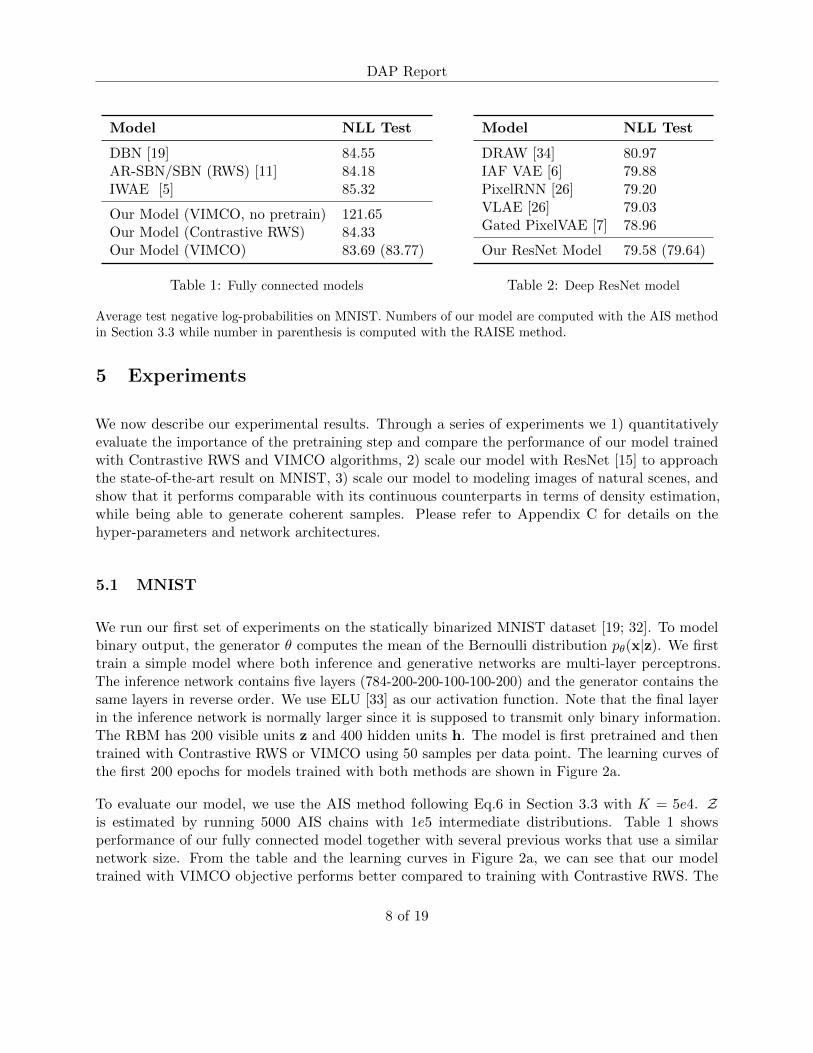
Model NLL Test
DBN [19] 84.55AR-SBN/SBN (RWS) [11] 84.18IWAE [5] 85.32
Our Model (VIMCO, no pretrain) 121.65Our Model (Contrastive RWS) 84.33Our Model (VIMCO) 83.69 (83.77)
Table 1: Fully connected models
Model NLL Test
DRAW [34] 80.97IAF VAE [6] 79.88PixelRNN [26] 79.20VLAE [26] 79.03Gated PixelVAE [7] 78.96
Our ResNet Model 79.58 (79.64)
Table 2: Deep ResNet model
Average test negative log-probabilities on MNIST. Numbers of our model are computed with the AIS methodin Section 3.3 while number in parenthesis is computed with the RAISE method.
5 Experiments
We now describe our experimental results. Through a series of experiments we 1) quantitativelyevaluate the importance of the pretraining step and compare the performance of our model trainedwith Contrastive RWS and VIMCO algorithms, 2) scale our model with ResNet [15] to approachthe state-of-the-art result on MNIST, 3) scale our model to modeling images of natural scenes, andshow that it performs comparable with its continuous counterparts in terms of density estimation,while being able to generate coherent samples. Please refer to Appendix C for details on thehyper-parameters and network architectures.
5.1 MNIST
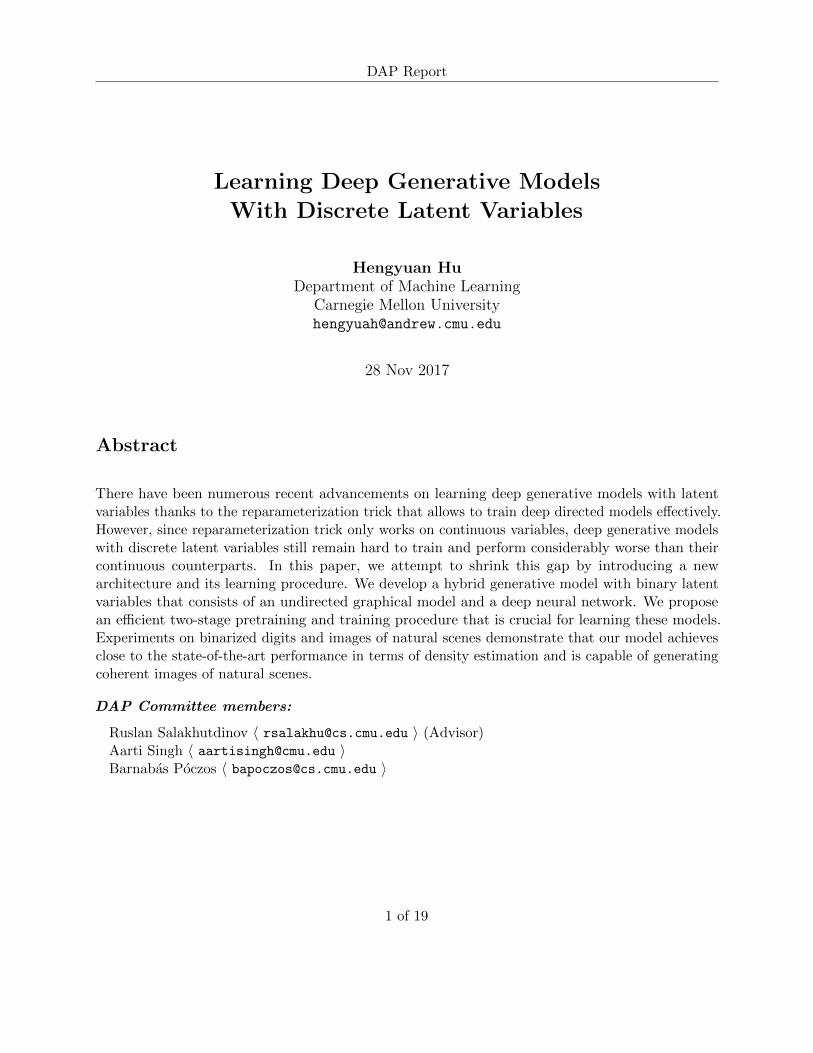
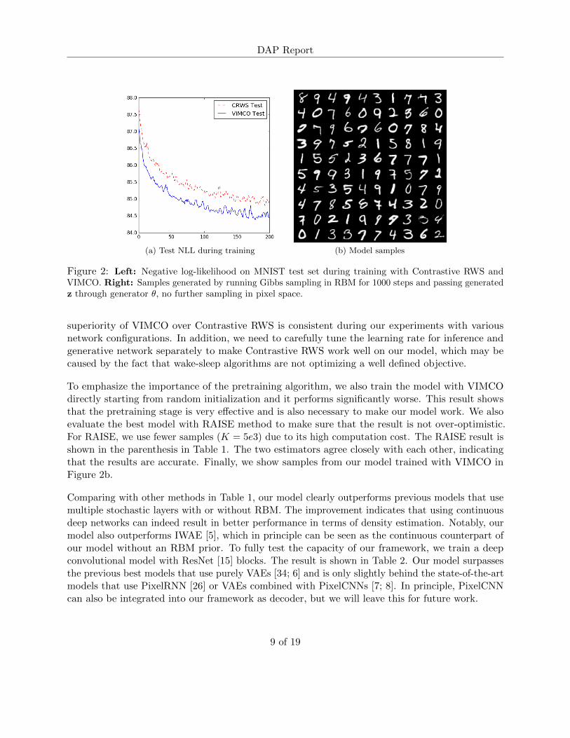
We run our first set of experiments on the statically binarized MNIST dataset [19; 32]. To modelbinary output, the generator θ computes the mean of the Bernoulli distribution pθ(x|z). We firsttrain a simple model where both inference and generative networks are multi-layer perceptrons.The inference network contains five layers (784-200-200-100-100-200) and the generator contains thesame layers in reverse order. We use ELU [33] as our activation function. Note that the final layerin the inference network is normally larger since it is supposed to transmit only binary information.The RBM has 200 visible units z and 400 hidden units h. The model is first pretrained and thentrained with Contrastive RWS or VIMCO using 50 samples per data point. The learning curves ofthe first 200 epochs for models trained with both methods are shown in Figure 2a.
To evaluate our model, we use the AIS method following Eq.6 in Section 3.3 with K = 5e4. Zis estimated by running 5000 AIS chains with 1e5 intermediate distributions. Table 1 showsperformance of our fully connected model together with several previous works that use a similarnetwork size. From the table and the learning curves in Figure 2a, we can see that our modeltrained with VIMCO objective performs better compared to training with Contrastive RWS. The
8 of 19
DAP Report
(a) Test NLL during training (b) Model samples
Figure 2: Left: Negative log-likelihood on MNIST test set during training with Contrastive RWS andVIMCO. Right: Samples generated by running Gibbs sampling in RBM for 1000 steps and passing generatedz through generator θ, no further sampling in pixel space.
superiority of VIMCO over Contrastive RWS is consistent during our experiments with variousnetwork configurations. In addition, we need to carefully tune the learning rate for inference andgenerative network separately to make Contrastive RWS work well on our model, which may becaused by the fact that wake-sleep algorithms are not optimizing a well defined objective.
To emphasize the importance of the pretraining algorithm, we also train the model with VIMCOdirectly starting from random initialization and it performs significantly worse. This result showsthat the pretraining stage is very effective and is also necessary to make our model work. We alsoevaluate the best model with RAISE method to make sure that the result is not over-optimistic.For RAISE, we use fewer samples (K = 5e3) due to its high computation cost. The RAISE result isshown in the parenthesis in Table 1. The two estimators agree closely with each other, indicatingthat the results are accurate. Finally, we show samples from our model trained with VIMCO inFigure 2b.
Comparing with other methods in Table 1, our model clearly outperforms previous models that usemultiple stochastic layers with or without RBM. The improvement indicates that using continuousdeep networks can indeed result in better performance in terms of density estimation. Notably, ourmodel also outperforms IWAE [5], which in principle can be seen as the continuous counterpart ofour model without an RBM prior. To fully test the capacity of our framework, we train a deepconvolutional model with ResNet [15] blocks. The result is shown in Table 2. Our model surpassesthe previous best models that use purely VAEs [34; 6] and is only slightly behind the state-of-the-artmodels that use PixelRNN [26] or VAEs combined with PixelCNNs [7; 8]. In principle, PixelCNNcan also be integrated into our framework as decoder, but we will leave this for future work.
9 of 19
DAP Report
Model NLL Train NLL Test
ResNet VAE with IAF [6] 3.11DenseNet VLAE [7] 2.95PixelCNN++ [29] 2.92
IWAE 4.45 4.54Our Model (1024-2048) 4.73 4.84Our Model (2048-4096) 4.49 4.56
Table 3: Average test negative log-probabilities on CIFAR10 in bits/dim. Numbers of our model arecomputed with the AIS method.
5.2 CIFAR10
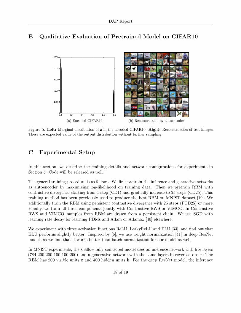
CIFAR10 has been a challenging benchmark for generative modeling. To model real value pixeldata, we set the generative distribution pθ(x|z) to be discretized logistic mixture following [29].In the pretraining stage, the objective is to minimize the negative log-likelihood. The marginaldistribution of the encoded z space and the reconstruction of test images are shown in Figure 5 inAppendix B. We note that the pretrained autoencoder preserves enough information while convertinghigh dimensional real value data to binary. This transformation makes it possible apply simplemodels like RBM to challenging tasks such as modeling CIFAR10 images. We train two modelsunder our framework. Both of them use ResNets [15] for inference and generative networks. Thelatent space for the first model has 1024 dimensions and is modeled by RBM with 2048 hiddenunits. The latent space for the second model has 2048 dimensions and RBM has 4096 hidden units.Similar to what we have discovered during the MNIST experiments, we find that VIMCO is moreeffective and robust to hyperparameters than Contrastive RWS. Therefore, the model is trainedusing VIMCO with 10 samples per data point.
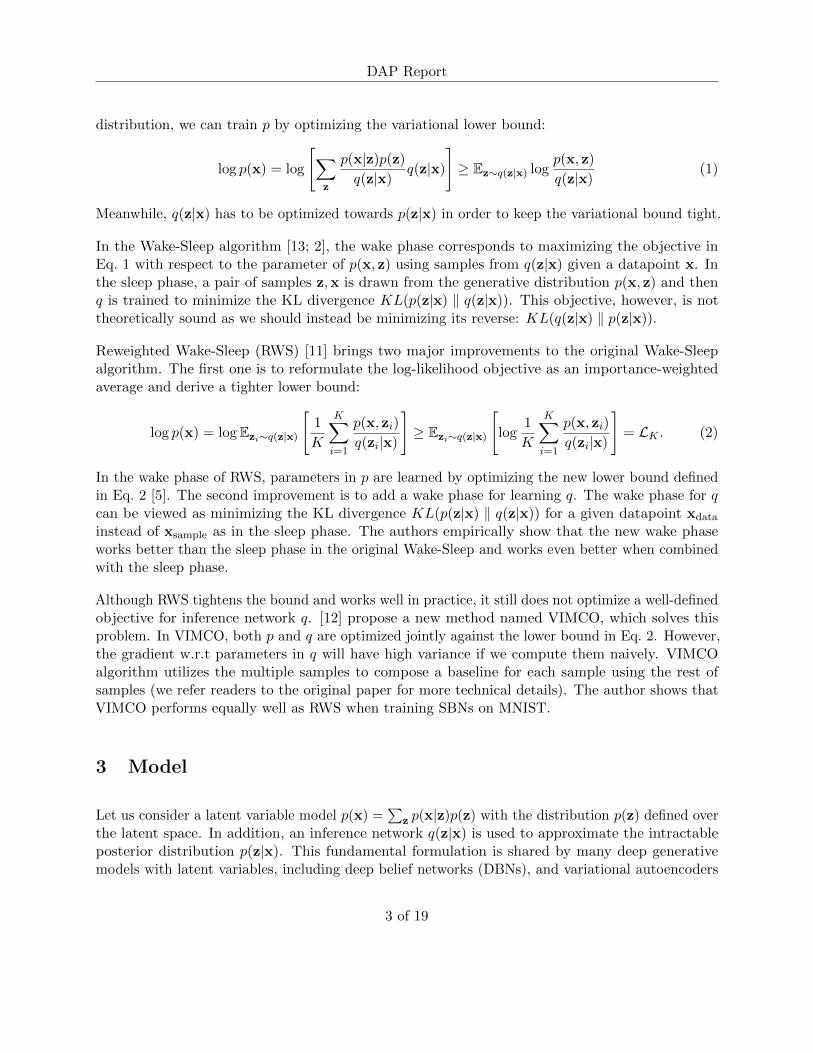
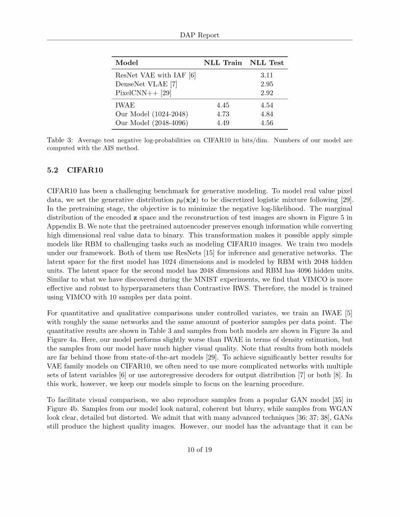
For quantitative and qualitative comparisons under controlled variates, we train an IWAE [5]with roughly the same networks and the same amount of posterior samples per data point. Thequantitative results are shown in Table 3 and samples from both models are shown in Figure 3a andFigure 4a. Here, our model performs slightly worse than IWAE in terms of density estimation, butthe samples from our model have much higher visual quality. Note that results from both modelsare far behind those from state-of-the-art models [29]. To achieve significantly better results forVAE family models on CIFAR10, we often need to use more complicated networks with multiplesets of latent variables [6] or use autoregressive decoders for output distribution [7] or both [8]. Inthis work, however, we keep our models simple to focus on the learning procedure.
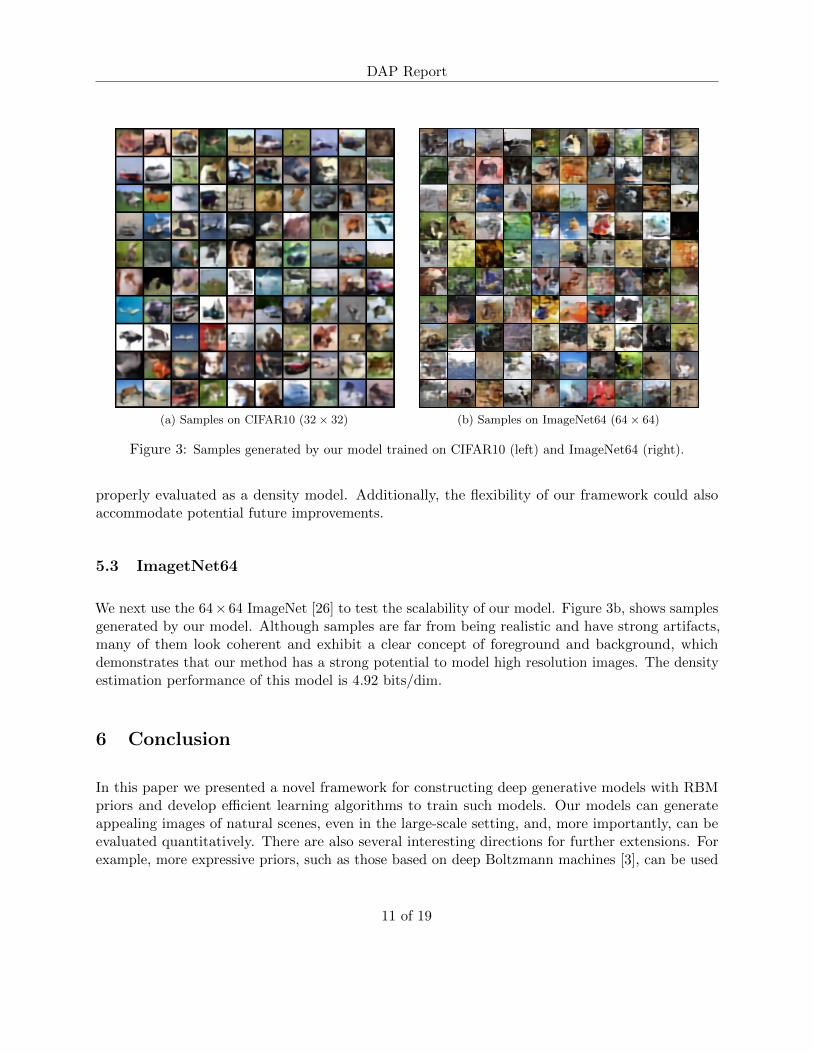
To facilitate visual comparison, we also reproduce samples from a popular GAN model [35] inFigure 4b. Samples from our model look natural, coherent but blurry, while samples from WGANlook clear, detailed but distorted. We admit that with many advanced techniques [36; 37; 38], GANsstill produce the highest quality images. However, our model has the advantage that it can be
10 of 19
DAP Report
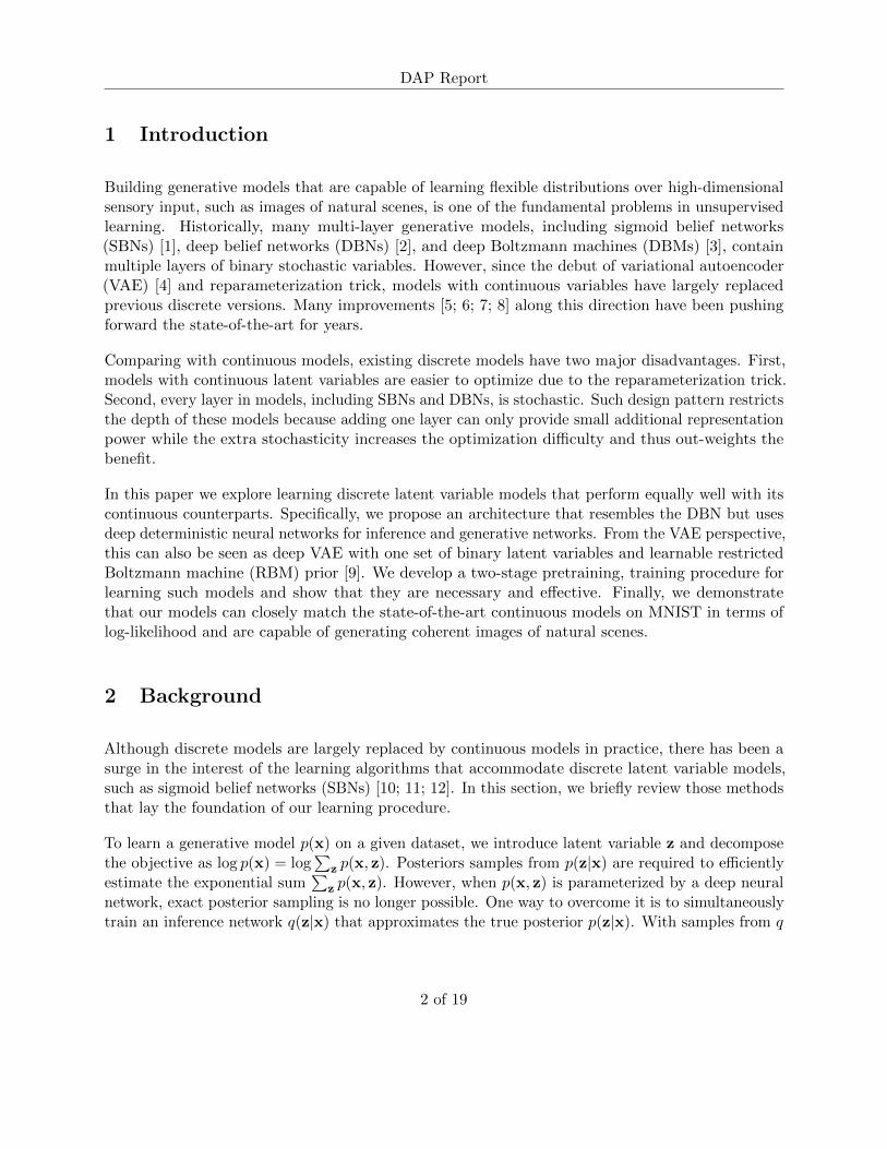
(a) Samples on CIFAR10 (32× 32) (b) Samples on ImageNet64 (64× 64)
Figure 3: Samples generated by our model trained on CIFAR10 (left) and ImageNet64 (right).
properly evaluated as a density model. Additionally, the flexibility of our framework could alsoaccommodate potential future improvements.
5.3 ImagetNet64
We next use the 64× 64 ImageNet [26] to test the scalability of our model. Figure 3b, shows samplesgenerated by our model. Although samples are far from being realistic and have strong artifacts,many of them look coherent and exhibit a clear concept of foreground and background, whichdemonstrates that our method has a strong potential to model high resolution images. The densityestimation performance of this model is 4.92 bits/dim.
6 Conclusion
In this paper we presented a novel framework for constructing deep generative models with RBMpriors and develop efficient learning algorithms to train such models. Our models can generateappealing images of natural scenes, even in the large-scale setting, and, more importantly, can beevaluated quantitatively. There are also several interesting directions for further extensions. Forexample, more expressive priors, such as those based on deep Boltzmann machines [3], can be used
11 of 19
DAP Report
(a) Samples on CIFAR10 from IWAE (b) Samples from WGAN
Figure 4: Samples generated by IWAE (left) and WGAN (right) trained on CIFAR10
in place of RBMs, while autoregressive [39] or recurrent networks [26] can be used for inference andgenerative networks.
References
[1] R. M. Neal, “Connectionist learning of belief networks,” Artif. Intell., vol. 56, no. 1, pp. 71–113, Jul.1992. [Online]. Available: http://dx.doi.org/10.1016/0004-3702(92)90065-6
[2] G. E. Hinton, S. Osindero, and Y.-W. Teh, “A fast learning algorithm for deep beliefnets,” Neural Comput., vol. 18, no. 7, pp. 1527–1554, Jul. 2006. [Online]. Available:http://dx.doi.org/10.1162/neco.2006.18.7.1527
[3] R. Salakhutdinov and G. E. Hinton, “Deep boltzmann machines,” in Proceedings of theTwelfth International Conference on Artificial Intelligence and Statistics, AISTATS 2009,Clearwater Beach, Florida, USA, April 16-18, 2009, 2009, pp. 448–455. [Online]. Available:http://www.jmlr.org/proceedings/papers/v5/salakhutdinov09a.html
[4] D. P. Kingma and M. Welling, “Auto-Encoding Variational Bayes,” ArXiv e-prints, Dec. 2013.
[5] Y. Burda, R. B. Grosse, and R. Salakhutdinov, “Importance weighted autoencoders,” CoRR, vol.abs/1509.00519, 2015. [Online]. Available: http://arxiv.org/abs/1509.00519
[6] D. P. Kingma, T. Salimans, and M. Welling, “Improving variational inference with inverse autoregressiveflow,” CoRR, vol. abs/1606.04934, 2016. [Online]. Available: http://arxiv.org/abs/1606.04934
12 of 19
DAP Report
[7] X. Chen, D. P. Kingma, T. Salimans, Y. Duan, P. Dhariwal, J. Schulman, I. Sutskever, andP. Abbeel, “Variational lossy autoencoder,” CoRR, vol. abs/1611.02731, 2016. [Online]. Available:http://arxiv.org/abs/1611.02731
[8] I. Gulrajani, K. Kumar, F. Ahmed, A. A. Taiga, F. Visin, D. Vazquez, and A. C. Courville, “Pixelvae:A latent variable model for natural images,” CoRR, vol. abs/1611.05013, 2016. [Online]. Available:http://arxiv.org/abs/1611.05013
[9] G. E. Hinton, “Training products of experts by minimizing contrastive divergence,” NeuralComput., vol. 14, no. 8, pp. 1771–1800, Aug. 2002. [Online]. Available: http://dx.doi.org/10.1162/089976602760128018
[10] A. Mnih and K. Gregor, “Neural variational inference and learning in belief networks,” CoRR, vol.abs/1402.0030, 2014. [Online]. Available: http://arxiv.org/abs/1402.0030
[11] J. Bornschein and Y. Bengio, “Reweighted wake-sleep,” CoRR, vol. abs/1406.2751, 2014. [Online].Available: http://arxiv.org/abs/1406.2751
[12] A. Mnih and D. J. Rezende, “Variational inference for monte carlo objectives,” CoRR, vol.abs/1602.06725, 2016. [Online]. Available: http://arxiv.org/abs/1602.06725
[13] G. E. Hinton, P. Dayan, B. J. Frey, and R. M. Neal, “The wake-sleep algorithm for unsupervised neuralnetworks,” Science, vol. 268, pp. 1158–1161, 1995.
[14] N. Srivastava, G. Hinton, A. Krizhevsky, I. Sutskever, and R. Salakhutdinov, “Dropout: A simpleway to prevent neural networks from overfitting,” Journal of Machine Learning Research, vol. 15, pp.1929–1958, 2014. [Online]. Available: http://jmlr.org/papers/v15/srivastava14a.html
[15] K. He, X. Zhang, S. Ren, and J. Sun, “Deep residual learning for image recognition,” CoRR, vol.abs/1512.03385, 2015. [Online]. Available: http://arxiv.org/abs/1512.03385
[16] G. Huang, Z. Liu, and K. Q. Weinberger, “Densely connected convolutional networks,” CoRR, vol.abs/1608.06993, 2016. [Online]. Available: http://arxiv.org/abs/1608.06993
[17] J. Balle, V. Laparra, and E. P. Simoncelli, “End-to-end optimized image compression,” CoRR, vol.abs/1611.01704, 2016. [Online]. Available: http://arxiv.org/abs/1611.01704
[18] T. Tieleman, “Training restricted boltzmann machines using approximations to the likelihood gradient,”in Proceedings of the 25th International Conference on Machine Learning, ser. ICML ’08. New York,NY, USA: ACM, 2008, pp. 1064–1071. [Online]. Available: http://doi.acm.org/10.1145/1390156.1390290
[19] R. Salakhutdinov and I. Murray, “On the quantitative analysis of deep belief networks,” in Proceedingsof the 25th International Conference on Machine Learning, ser. ICML ’08. New York, NY, USA: ACM,2008, pp. 872–879. [Online]. Available: http://doi.acm.org/10.1145/1390156.1390266
[20] Y. Burda, R. B. Grosse, and R. Salakhutdinov, “Accurate and conservative estimates of MRFlog-likelihood using reverse annealing,” CoRR, vol. abs/1412.8566, 2014. [Online]. Available:http://arxiv.org/abs/1412.8566
[21] J. Ngiam, Z. Chen, P. W. Koh, and A. Y. Ng, “Learning deep energy models.” inICML, L. Getoor and T. Scheffer, Eds. Omnipress, 2011, pp. 1105–1112. [Online]. Available:http://dblp.uni-trier.de/db/conf/icml/icml2011.html#NgiamCKN11
13 of 19
DAP Report
[22] H. Lee, R. Grosse, R. Ranganath, and A. Y. Ng, “Convolutional deep belief networks for scalableunsupervised learning of hierarchical representations,” in Proceedings of the 26th Annual InternationalConference on Machine Learning, ser. ICML ’09. New York, NY, USA: ACM, 2009, pp. 609–616.[Online]. Available: http://doi.acm.org/10.1145/1553374.1553453
[23] Z. Yang, Z. Hu, R. Salakhutdinov, and T. Berg-Kirkpatrick, “Improved variational autoencodersfor text modeling using dilated convolutions,” CoRR, vol. abs/1702.08139, 2017. [Online]. Available:http://arxiv.org/abs/1702.08139
[24] Y. Pu, Z. Gan, R. Henao, X. Yuan, C. Li, A. Stevens, and L. Carin, “Variational Autoencoder for DeepLearning of Images, Labels and Captions,” ArXiv e-prints, Sep. 2016.
[25] D. Jimenez Rezende and S. Mohamed, “Variational Inference with Normalizing Flows,” ArXiv e-prints,May 2015.
[26] A. van den Oord, N. Kalchbrenner, and K. Kavukcuoglu, “Pixel recurrent neural networks,” CoRR, vol.abs/1601.06759, 2016. [Online]. Available: http://arxiv.org/abs/1601.06759
[27] I. J. Goodfellow, J. Pouget-Abadie, M. Mirza, B. Xu, D. Warde-Farley, S. Ozair, A. Courville, andY. Bengio, “Generative Adversarial Networks,” ArXiv e-prints, Jun. 2014.
[28] A. van den Oord, N. Kalchbrenner, O. Vinyals, L. Espeholt, A. Graves, and K. Kavukcuoglu,“Conditional image generation with pixelcnn decoders,” CoRR, vol. abs/1606.05328, 2016. [Online].Available: http://arxiv.org/abs/1606.05328
[29] T. Salimans, A. Karpathy, X. Chen, and D. P. Kingma, “Pixelcnn++: Improving the pixelcnn withdiscretized logistic mixture likelihood and other modifications,” CoRR, vol. abs/1701.05517, 2017.[Online]. Available: http://arxiv.org/abs/1701.05517
[30] L. Theis, A. van den Oord, and M. Bethge, “A note on the evaluation of generative models,” ArXive-prints, Nov. 2015.
[31] Y. Wu, Y. Burda, R. Salakhutdinov, and R. B. Grosse, “On the quantitative analysisof decoder-based generative models,” CoRR, vol. abs/1611.04273, 2016. [Online]. Available:http://arxiv.org/abs/1611.04273
[32] H. Larochelle and I. Murray, “The neural autoregressive distribution estimator,” in The Proceedings ofthe 14th International Conference on Artificial Intelligence and Statistics, ser. JMLR: W&CP, vol. 15,2011, pp. 29–37.
[33] D. Clevert, T. Unterthiner, and S. Hochreiter, “Fast and accurate deep network learningby exponential linear units (elus),” CoRR, vol. abs/1511.07289, 2015. [Online]. Available:http://arxiv.org/abs/1511.07289
[34] K. Gregor, I. Danihelka, A. Graves, and D. Wierstra, “DRAW: A recurrent neural network for imagegeneration,” CoRR, vol. abs/1502.04623, 2015. [Online]. Available: http://arxiv.org/abs/1502.04623
[35] M. Arjovsky, S. Chintala, and L. Bottou, “Wasserstein GAN,” ArXiv e-prints, Jan. 2017.
[36] T. Salimans, I. J. Goodfellow, W. Zaremba, V. Cheung, A. Radford, and X. Chen,“Improved techniques for training gans,” CoRR, vol. abs/1606.03498, 2016. [Online]. Available:http://arxiv.org/abs/1606.03498
14 of 19
DAP Report
[37] S. Arora, R. Ge, Y. Liang, T. Ma, and Y. Zhang, “Generalization and equilibrium in generative adversarialnets (gans),” CoRR, vol. abs/1703.00573, 2017. [Online]. Available: http://arxiv.org/abs/1703.00573
[38] Z. Dai, A. Almahairi, P. Bachman, E. H. Hovy, and A. C. Courville, “Calibrating energy-based generative adversarial networks,” CoRR, vol. abs/1702.01691, 2017. [Online]. Available:http://arxiv.org/abs/1702.01691
[39] K. Gregor, A. Mnih, and D. Wierstra, “Deep autoregressive networks,” CoRR, vol. abs/1310.8499, 2013.[Online]. Available: http://arxiv.org/abs/1310.8499
[40] D. P. Kingma and J. Ba, “Adam: A method for stochastic optimization,” CoRR, vol. abs/1412.6980,2014. [Online]. Available: http://arxiv.org/abs/1412.6980
[41] T. Salimans and D. P. Kingma, “Weight normalization: A simple reparameterization toaccelerate training of deep neural networks,” CoRR, vol. abs/1602.07868, 2016. [Online]. Available:http://arxiv.org/abs/1602.07868
[42] K. He, X. Zhang, S. Ren, and J. Sun, “Identity mappings in deep residual networks,” CoRR, vol.abs/1603.05027, 2016. [Online]. Available: http://arxiv.org/abs/1603.05027
[43] A. Odena, V. Dumoulin, and C. Olah, “Deconvolution and checkerboard artifacts,” Distill, 2016.[Online]. Available: http://distill.pub/2016/deconv-checkerboard
15 of 19
DAP Report
A Details on Contrastive Reweighted Wake-Sleep and VIMCO
A.1 Contrastive Reweighted Wake-Sleep
Algorithm 1 Contrastive Reweighted Wake-Sleep for a single observation
1: Sample x from training distribution.2: for i = 1 to K do3: Sample zi from qφ(z|x).4: end for5: Compute unnormalized weights wi =
p∗θ(x,zi)qφ(zi|x)
6: Normalize the weights wi = wi∑i′ wi′
7: Sample {z−} from M CD/PCD chains and pass through generator θ to obtain {x−}8: Wake update for generative network θ with gradient:
K∑i=1
wi∇θ log pθ(x, zi)
9: Wake and sleep updates for inference network φ with gradient:
K∑i=1
wi∇φ log qφ(z(k)|x) +1
M
M∑j=1
∇φ log qφ(z−j |x−j )
10: Update RBM ϕ with gradient:
−K∑i=1
wi∇ϕFϕ(zi) +1
M
M∑j=1
∇ϕFϕ(z−j )
16 of 19
DAP Report
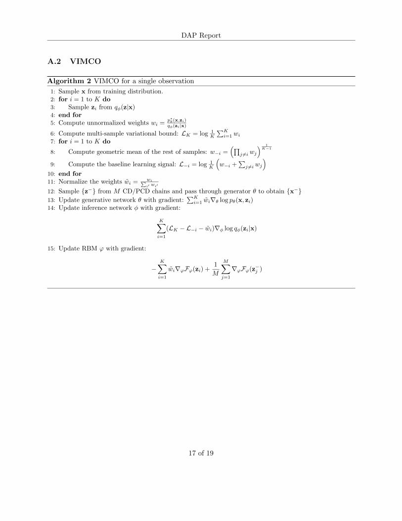
A.2 VIMCO
Algorithm 2 VIMCO for a single observation
1: Sample x from training distribution.2: for i = 1 to K do3: Sample zi from qφ(z|x)4: end for5: Compute unnormalized weights wi =
p∗θ(x,zi)qφ(zi|x)
6: Compute multi-sample variational bound: LK = log 1K
∑Ki=1 wi
7: for i = 1 to K do
8: Compute geometric mean of the rest of samples: w−i =(∏
j 6=i wj
) 1K−1
9: Compute the baseline learning signal: L−i = log 1K
(w−i +
∑j 6=i wj
)10: end for11: Normalize the weights wi = wi∑
i′ wi′
12: Sample {z−} from M CD/PCD chains and pass through generator θ to obtain {x−}13: Update generative network θ with gradient:
∑Ki=1 wi∇θ log pθ(x, zi)
14: Update inference network φ with gradient:
K∑i=1
(LK − L−i − wi)∇φ log qφ(zi|x)
15: Update RBM ϕ with gradient:
−K∑i=1
wi∇ϕFϕ(zi) +1
M
M∑j=1
∇ϕFϕ(z−j )
17 of 19
DAP Report
B Qualitative Evaluation of Pretrained Model on CIFAR10
(a) Encoded CIFAR10 (b) Reconstruction by autoencoder
Figure 5: Left: Marginal distribution of z in the encoded CIFAR10. Right: Reconstruction of test images.These are expected value of the output distribution without further sampling.
C Experimental Setup
In this section, we describe the training details and network configurations for experiments inSection 5. Code will be released as well.
The general training procedure is as follows. We first pretrain the inference and generative networksas autoencoder by maximizing log-likelihood on training data. Then we pretrain RBM withcontrastive divergence starting from 1 step (CD1) and gradually increase to 25 steps (CD25). Thistraining method has been previously used to produce the best RBM on MNIST dataset [19]. Weadditionally train the RBM using persistent contrastive divergence with 25 steps (PCD25) or more.Finally, we train all three components jointly with Contrastive RWS or VIMCO. In ContrastiveRWS and VIMCO, samples from RBM are drawn from a persistent chain. We use SGD withlearning rate decay for learning RBMs and Adam or Adamax [40] elsewhere.
We experiment with three activation functions ReLU, LeakyReLU and ELU [33], and find out thatELU performs slightly better. Inspired by [6], we use weight normalization [41] in deep ResNetmodels as we find that it works better than batch normalization for our model as well.
In MNIST experiments, the shallow fully connected model uses an inference network with five layers(784-200-200-100-100-200) and a generative network with the same layers in reversed order. TheRBM has 200 visible units z and 400 hidden units h. For the deep ResNet model, the inference
18 of 19
DAP Report
network uses three basic pre-activation [42] residual blocks with 25, 50, 50 feature maps. Each blockuses kernel size 3 and is repeated twice with stride 2 and 1 respectively. After residual blocks, thereis a fully connected layer with 200 neurons. The RBM has 200 visible units and 400 hidden units.The generative network uses the same blocks but with stride one. We upsample the feature mapwith nearest neighbour interpolation by a factor of 2 before feeding it into each block and shortcutto avoid checkerboard artifact [43].
In CIFAR10 and ImageNet64 experiments, the output distribution pθ is a discretized mixture of 10logistic distributions [29]. The network for CIFAR10 uses 4 residual blocks with 64, 128, 192, 256feature maps. Each block is repeated twice as in MNIST. There is no fully connected layer in thismodel and final feature map (256× 2× 2) is flattened to a 1024 dimensional vector. The RBM has1024 visible units and 2048 hidden units. The network for ImageNet64 uses 5 residual blocks with64, 128, 128, 256, 256 feature maps. Each block uses stride 2 and is only repeated once. The RBMis the same as the one in CIFAR10.
19 of 19