Learning Dynamic Routing for Semantic Segmentation

Yanwei Li1,2, Lin Song3, Yukang Chen1,2, Zeming Li4, Xiangyu Zhang4,

Xingang Wang1, Jian Sun4

1Institute of Automation, Chinese Academy of Sciences2University of Chinese Academy of Sciences

3Xi’an Jiaotong University 4Megvii Technology

Abstract

Recently, numerous handcrafted and searched networks

have been applied for semantic segmentation. However,

previous works intend to handle inputs with various scales

in pre-defined static architectures, such as FCN, U-Net, and

DeepLab series. This paper studies a conceptually new

method to alleviate the scale variance in semantic represen-

tation, named dynamic routing. The proposed framework

generates data-dependent routes, adapting to the scale dis-

tribution of each image. To this end, a differentiable gating

function, called soft conditional gate, is proposed to select

scale transform paths on the fly. In addition, the computa-

tional cost can be further reduced in an end-to-end manner

by giving budget constraints to the gating function. We fur-

ther relax the network level routing space to support multi-

path propagations and skip-connections in each forward,

bringing substantial network capacity. To demonstrate the

superiority of the dynamic property, we compare with sev-

eral static architectures, which can be modeled as special

cases in the routing space. Extensive experiments are con-

ducted on Cityscapes and PASCAL VOC 2012 to illustrate

the effectiveness of the dynamic framework. Code is avail-

able at https://github.com/yanwei-li/DynamicRouting.1

1. Introduction

Semantic segmentation, which aims at assigning each

pixel with semantic categories, is one of the most funda-

mental yet challenging tasks in the computer vision field.

One of the problems in semantic segmentation comes from

the huge scale variance among inputs, e.g., the tiny object

instances and the picture-filled background stuff. More-

over, the large distribution variance brings difficulties to

feature representation as well as relationship modeling. Tra-

ditional methods try to solve this problem by well-designed

network architectures. For instance, multi-resolution fu-

1Work was done in Megvii Research. Email: liyanwei2017@ia.ac.cn

Input OutputOutput

(a) Network architecture of large-scale input

Input OutputOutput

(b) Network architecture of small-scale input

Input OutputOutput

(c) Network architecture of mixed-scale input

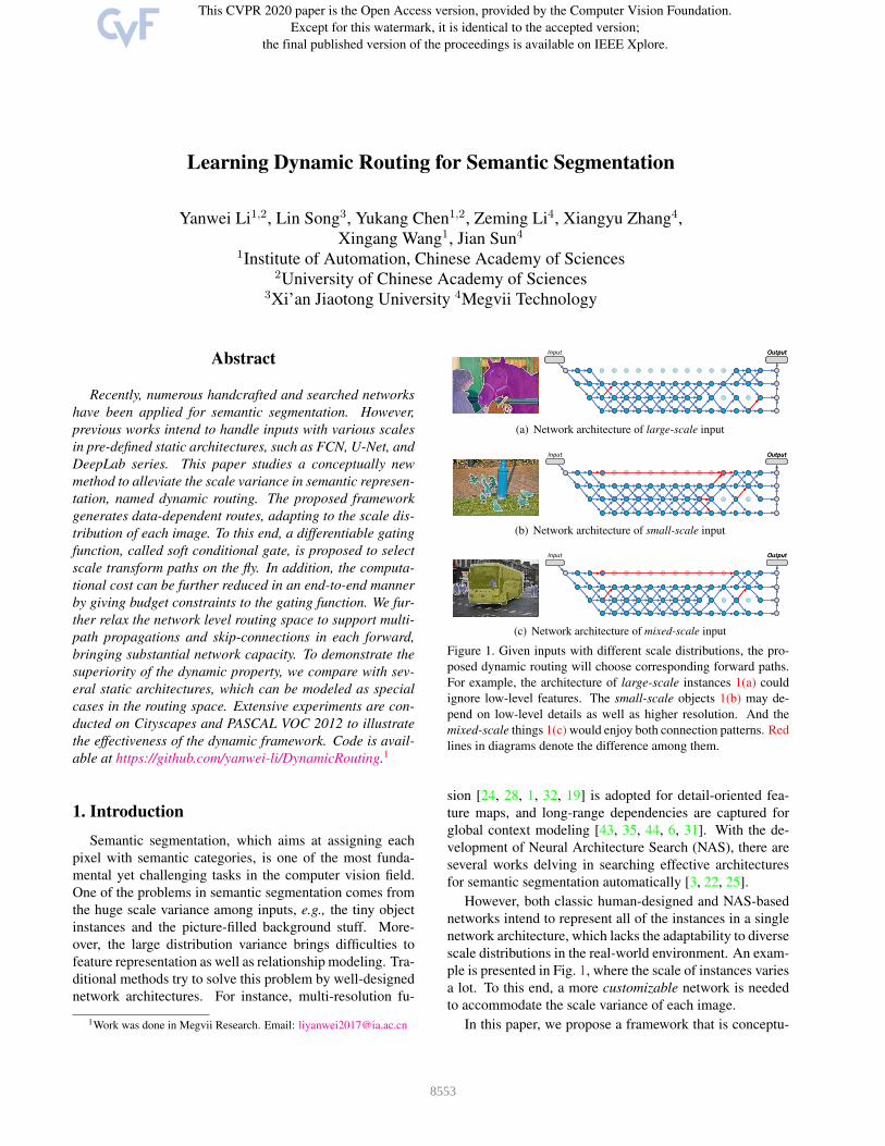
Figure 1. Given inputs with different scale distributions, the pro-

posed dynamic routing will choose corresponding forward paths.

For example, the architecture of large-scale instances 1(a) could

ignore low-level features. The small-scale objects 1(b) may de-

pend on low-level details as well as higher resolution. And the

mixed-scale things 1(c) would enjoy both connection patterns. Red

lines in diagrams denote the difference among them.

sion [24, 28, 1, 32, 19] is adopted for detail-oriented fea-

ture maps, and long-range dependencies are captured for

global context modeling [43, 35, 44, 6, 31]. With the de-

velopment of Neural Architecture Search (NAS), there are

several works delving in searching effective architectures

for semantic segmentation automatically [3, 22, 25].

However, both classic human-designed and NAS-based

networks intend to represent all of the instances in a single

network architecture, which lacks the adaptability to diverse

scale distributions in the real-world environment. An exam-

ple is presented in Fig. 1, where the scale of instances varies

a lot. To this end, a more customizable network is needed

to accommodate the scale variance of each image.

In this paper, we propose a framework that is conceptu-

8553

ally novel for semantic segmentation, called dynamic rout-

ing. In particular, the dynamic routing generates data-

dependent forward paths during inference, which means the

specific network architecture varies with inputs. With this

method, instances (or backgrounds) with different scales

could be allocated to corresponding resolution stages for

customized feature transformation. As illustrated in Fig. 1,

the input images with diverse scale distributions will choose

different routes for feature transformation. There are some

researches on dynamic networks for efficient object recog-

nition via dropping blocks [38, 17, 33, 36] or pruning chan-

nels [39, 20]. Different from them, this work focuses on

semantic representation and intends to alleviate scale vari-

ance as well as improve network efficiency.

The routing space in traditional dynamic approaches

for image classification [17, 33, 36] are usually limited

to a resolution declining pipeline, which would not suf-

fice for semantic segmentation. We draw inspiration from

the search space of Auto-DeepLab [22] and develop a

new routing space for better capacity, which contains sev-

eral independent cells. Specifically, different from Auto-

DeepLab, multi-path propagations and skip-connections,

which are proved to be quiet essential in semantic segmen-

tation [28, 6], are enabled in each forward during inference.

Therefore, several classic network architectures can be in-

cluded as special cases for comparisons (Fig. 3). In terms of

the dynamic routing, a data-dependent routing gate, called

soft conditional gate, is designed to select each path accord-

ing to the input image. With the proposed routing gate, each

basic cell, as well as the resolution transformation path, can

be taken into consideration individually. Moreover, the pro-

posed routing gate can be formulated into a differentiable

module for end-to-end optimization. Consequently, given

limited computational budgets (e.g., FLOPs), cells with lit-

tle contribution will be dropped on the fly.

The overall approach, named dynamic routing, can be

easily instantiated for semantic segmentation. To elaborate

on its superiority over the fixed architectures in both per-

formance and efficiency, we give extensive ablation stud-

ies and detailed analyses in Sec. 4.3. Experimental results

are further reported on two well-known datasets, namely

Cityscapes [9] and PASCAL VOC 2012 [11]. With the

simple scale transformation modules, the proposed dynamic

routing achieves comparable results with the state-of-the-art

methods but consumes much fewer resources.

2. Related Works

Traditional semantic segmentation researches mainly fo-

cused on designing subtle network architectures by human

experiences [24, 28, 1, 43, 6]. With the development of

NAS, there are several methods attempting to search for a

static network automatically [3, 22, 25]. Unlike previous

works, the dynamic routing is proposed to select the most

suitable scale transform according to the input, which has

seldom been explored. Herein, we first retrospect hand-

designed architectures for semantic segmentation. Then we

give an introduction to NAS-based approaches. Finally, pre-

vious developments of dynamic networks are reviewed.

2.1. Handcrafted Architectures

Handcrafted architectures have been well studied in re-

cent years. There are several researches delving in net-

work design for semantic segmentation, e.g., FCN [24], U-

Net [28], Conv-Deconv [26], SegNet [1]. Based on the well-

designed FCN [24] and U-shape architecture [28], numer-

ous works have been proposed to model global context by

capturing larger receptive field [43, 4, 5, 6, 41] or estab-

lishing pixel-wise relationships [44, 18, 12, 31]. Due to the

high resource consumption of dense prediction, some light-

weighted architectures have been proposed for the sake of

efficiency, including ICNet [42] and BiSeNet [40]. Overall,

handcrafted architectures aim at utilizing multi-scale fea-

tures from different stages in a static network, rather than

adapting to input dynamically.

2.2. NAS­based Approaches

Recently, Neural Architecture Search (NAS) has been

widely used for automatic network architecture design [45,

27, 23, 2, 13, 7]. When it comes to the specific domain,

there are several approaches trying to search for effective

architectures that are more suitable for semantic segmenta-

tion. Specifically, Chen et.al. [3] searches for multi-scale

module to replace ASPP [5] block. Furthermore, Nekrasov

et.al. [25] studies the routing type of auxiliary cells in

the decoder using the NAS-based method. More recently,

Auto-DeepLab [22] is proposed to search for a single route

from the dense-connected search space. Different from the

NAS-based approaches, which search for a single architec-

ture and then retrain it, the proposed dynamic routing gen-

erates forward paths on the fly without searching.

2.3. Dynamic Networks

Dynamic networks, adjusting the network architecture to

the corresponding input, have been recently studied in the

computer vision domain. Traditional methods mainly focus

on image classification by dropping blocks [38, 17, 33, 36]

or pruning channels [39, 20] for efficient inference. For ex-

ample, an early-existing strategy is adopted in MSDNet [17]

for resource-efficient object recognition, which classifies

easier inputs and gives output in earlier stages. And Skip-

Net [36] attempts to skip convolutional blocks using an RL-

based gating network. However, dynamic routing has sel-

dom been explored for scale transformation, especially in

semantic segmentation. To utilize the dynamic property, an

end-to-end dynamic routing framework is proposed in this

paper to alleviate the scale variance among inputs.

8554

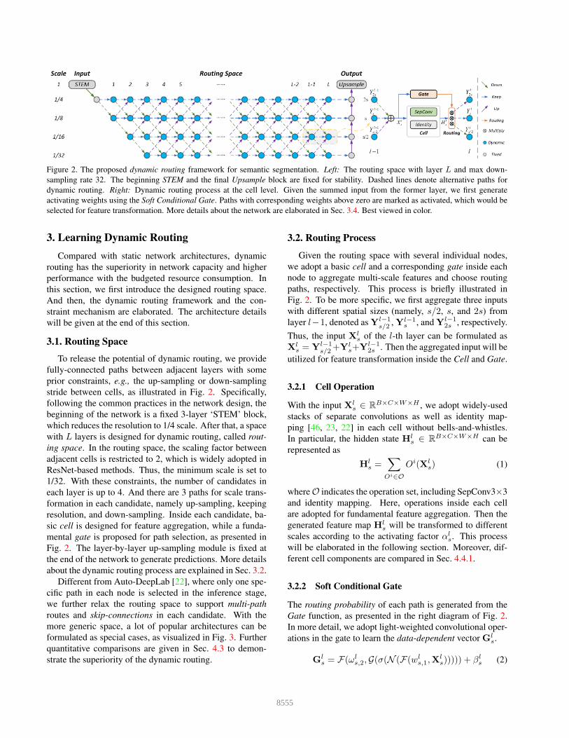
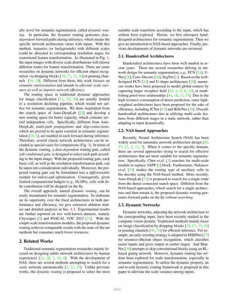
Figure 2. The proposed dynamic routing framework for semantic segmentation. Left: The routing space with layer L and max down-

sampling rate 32. The beginning STEM and the final Upsample block are fixed for stability. Dashed lines denote alternative paths for

dynamic routing. Right: Dynamic routing process at the cell level. Given the summed input from the former layer, we first generate

activating weights using the Soft Conditional Gate. Paths with corresponding weights above zero are marked as activated, which would be

selected for feature transformation. More details about the network are elaborated in Sec. 3.4. Best viewed in color.

3. Learning Dynamic Routing

Compared with static network architectures, dynamic

routing has the superiority in network capacity and higher

performance with the budgeted resource consumption. In

this section, we first introduce the designed routing space.

And then, the dynamic routing framework and the con-

straint mechanism are elaborated. The architecture details

will be given at the end of this section.

3.1. Routing Space

To release the potential of dynamic routing, we provide

fully-connected paths between adjacent layers with some

prior constraints, e.g., the up-sampling or down-sampling

stride between cells, as illustrated in Fig. 2. Specifically,

following the common practices in the network design, the

beginning of the network is a fixed 3-layer ‘STEM’ block,

which reduces the resolution to 1/4 scale. After that, a space

with L layers is designed for dynamic routing, called rout-

ing space. In the routing space, the scaling factor between

adjacent cells is restricted to 2, which is widely adopted in

ResNet-based methods. Thus, the minimum scale is set to

1/32. With these constraints, the number of candidates in

each layer is up to 4. And there are 3 paths for scale trans-

formation in each candidate, namely up-sampling, keeping

resolution, and down-sampling. Inside each candidate, ba-

sic cell is designed for feature aggregation, while a funda-

mental gate is proposed for path selection, as presented in

Fig. 2. The layer-by-layer up-sampling module is fixed at

the end of the network to generate predictions. More details

about the dynamic routing process are explained in Sec. 3.2.

Different from Auto-DeepLab [22], where only one spe-

cific path in each node is selected in the inference stage,

we further relax the routing space to support multi-path

routes and skip-connections in each candidate. With the

more generic space, a lot of popular architectures can be

formulated as special cases, as visualized in Fig. 3. Further

quantitative comparisons are given in Sec. 4.3 to demon-

strate the superiority of the dynamic routing.

3.2. Routing Process

Given the routing space with several individual nodes,

we adopt a basic cell and a corresponding gate inside each

node to aggregate multi-scale features and choose routing

paths, respectively. This process is briefly illustrated in

Fig. 2. To be more specific, we first aggregate three inputs

with different spatial sizes (namely, s/2, s, and 2s) from

layer l−1, denoted as Yl−1

s/2 , Yl−1s , and Y

l−1

2s , respectively.

Thus, the input Xls of the l-th layer can be formulated as

Xls = Y

l−1

s/2+Yls+Y

l−1

2s . Then the aggregated input will be

utilized for feature transformation inside the Cell and Gate.

3.2.1 Cell Operation

With the input Xls ∈ R

B×C×W×H , we adopt widely-used

stacks of separate convolutions as well as identity map-

ping [46, 23, 22] in each cell without bells-and-whistles.

In particular, the hidden state Hls ∈ R

B×C×W×H can be

represented as

Hls =

∑

Oi∈O

Oi(Xls) (1)

where O indicates the operation set, including SepConv3×3

and identity mapping. Here, operations inside each cell

are adopted for fundamental feature aggregation. Then the

generated feature map Hls will be transformed to different

scales according to the activating factor αls. This process

will be elaborated in the following section. Moreover, dif-

ferent cell components are compared in Sec. 4.4.1.

3.2.2 Soft Conditional Gate

The routing probability of each path is generated from the

Gate function, as presented in the right diagram of Fig. 2.

In more detail, we adopt light-weighted convolutional oper-

ations in the gate to learn the data-dependent vector Gls.

Gls = F(ωl

s,2,G(σ(N (F(wls,1,X

ls))))) + βl

s (2)

8555

STEM

OutputInput

Upsample

Routing Space

1 2 3 4 5 …... L-2 L-1 L

le

4

8

6

2

STEM

OutputInput

Upsample

Routing Space

1 2 3 4 5 …... L-2 L-1 L

le

4

8

6

2

…...…...

…...…...

…...…...

(a) Network architecture modeled from FCN-32s [24]

…...…...

STEM

OutputInput

Upsample

Routing Space

1 2 3 4 5 …... L-2 L-1 L

le

4

8

6

2

STEM

OutputInput

Upsample

Routing Space

1 2 3 4 5 …... L-2 L-1 L

le

4

8

6

2

…...…...

…...…...

(b) Network architecture modeled from U-Net [28]

…...…...

…...…...

STEM

OutputInput

Upsample

Routing Space

1 2 3 4 5 …... L-2 L-1 L

4

8

6

2

ASPP

le

STEM

OutputInput

Upsample

Routing Space

1 2 3 4 5 …... L-2 L-1 L

4

8

6

2

ASPP

le

…...…...

(c) Network architecture modeled from DeepLabV3 [5]

…...…...

…...…...

…...…...

…...…...

…...…...

…...…...

…...…...

STEM

OutputInput

Upsample

Routing Space

1 2 3 4 5 …... L-2 L-1 L

4

8

6

2

le

STEM

OutputInput

Upsample

Routing Space

1 2 3 4 5 …... L-2 L-1 L

4

8

6

2

le

(d) Network architecture modeled from HRNetV2 [32]

…...…...

…...…...

…...…...

STEM

OutputInput

Upsample

Routing Space

1 2 3 4 5 …... L-2 L-1 L

4

8

6

2

ASPP

le

STEM

OutputInput

Upsample

Routing Space

1 2 3 4 5 …... L-2 L-1 L

4

8

6

2

ASPP

le

(e) Network architecture modeled from Auto-DeepLab [22]

Figure 3. Sampled architectures from previous works. With

the designed routing space, several classic architectures can be

formulated in similar forms, e.g., FCN-32s 3(a), U-Net 3(b),

DeepLabV3 3(c), HRNetV2 3(d), and Auto-DeepLab 3(e).

where F(·, ·) denotes a convolutional function, σ indicates

ReLU activation, N and G represent batch normalization

and global average pooling respectively. Both ω and β are

convolutional parameters. Different from traditional RL-

based methods [36, 38, 34], which adopt policy gradient

to update the agent for discrete path selection, we propose

the soft conditional gate for differentiable routing. To this

end, with the feature vector Gls ∈ R

B×3×1×1, an activation

function δ is designed as

δ(·) = max(0,Tanh(·)) (3)

Therefore, the activating factor αls ∈ R

B×3×1×1 can be

calculated by δ(Gls), where αl

s belongs to [0, 1). When

αls→j = 0, the routing path from scale s to j will be

marked as closed. And all of the paths with αls→j > 0

will be reserved, enabling multi-path propagation. To be

more specific, the b-th input in batch B would generate cor-

responding αlb,s→j ∈ R

1×1×1×1, which means the routing

paths varies with inputs, or so called data-dependent. In

this way, each path can be taken into consideration individ-

ually, rather than only choose the relative important one for

propagation [23, 37, 22]. Furthermore, different activation

functions are investigated in Sec 4.4.2.

With the proposed activation function δ, the transform

from scale s to j ∈ {s/2, s, 2s} in the training process can

be formulated as

Ylj = αl

s→jTs→j(Hls) (4)

where Ts→j denotes the scale transformation (including up-

sampling, keeping resolution, and down-sampling) from

scale s to j. Therefore, with the activating factor αls, the pa-

rameters in Gls will be optimized during back-propagation

as long as one path is preserved (namely,∑

j αls→j > 0).

In the inference stage, if all of the paths are marked as

closed, the operations in Cell will be dropped to save com-

putational footprints. Recall from Eq. 1, this process is sum-

marized as

Hls =

{

Xls

∑

j αls→j = 0

∑

Oi∈O Oi(Xls)

∑

j αls→j > 0

(5)

Ylj =

0∑

jαls→j = 0, j 6= s

Hls

∑

j αls→j = 0, j = s

αls→jTs→j(H

ls)

∑

j αls→j > 0

(6)

3.3. Budget Constraint

Considering limited computational resources in the real-

world scene, we take the budget constraint into considera-

tion for efficient dynamic routing. Let us denote C as the

computational cost associated to the predefined operation,

e.g., FLOPs. Recall from Eq. 1, 2, and 4, we formulate the

expected cost inside the node in s-th scale and l-th layer as

C(Nodels) = C(Cellls) + C(Gatels) + C(Transls)

= max(αls)∑

Oi∈O C(Oi) + C(Gatels)+

∑

j αls→jC(Ts→j)

(7)

where Cellls, Gatels, and Transls indicates the functional op-

eration inside Cell, Gate, and Scale Transform, respectively.

Going one step further, the expected cost of the whole rout-

ing space could be calculated by

C(Space) =∑

l≤L

∑

s≤1/4

C(Nodels) (8)

Then we formulate the expected resource cost C(Space)into loss function LC for the end-to-end optimization:

LC = (C(Space)/C− µ)2

(9)

8556

where C represents the real resource cost of the whole rout-

ing space, and µ ∈ [0, 1] indicates the designed attenuation

factor. With different µ, the selected routes in each propa-

gation would be adaptively restricted to corresponding bud-

gets. The network performance under different budget con-

straints will be discussed in Sec. 4.4.3.

Overall, the network weights, as well as the soft condi-

tional gates, can be optimized with a joint loss function Lin a unified framework.

L = λ1LN + λ2LC (10)

where LN and LC denotes loss function of the whole net-

work and resource cost, respectively. λ1 and λ2 are utilized

to balance the optimization process of network prediction

and resource cost expectation, respectively.

3.4. Architecture Details

From a macro perspective, we set the depth of routing

space to 16 or 33 which is identical with that in widely-used

ResNet-50 and ResNet-101 [16], namely the total layer

L = 16 or 33 in Fig. 2. This setting brings convenience

to compare with the ResNet-based networks, which could

be formulated using the proposed routing space directly.

When it comes to micro nodes in the network, we adopt

three SepConv3×3 in the ‘STEM’ block, where the number

of filters is 64 for all of the convolutions. A stride 2 Conv1×1 is used for all of the s → s/2 paths, both to reduce feature

resolution and double the number of filters. And Conv1× 1followed by bilinear up-sampling is adopted for all of the

s → 2s connections, both to increase spatial resolution as

well as halve the number of filters.

Moreover, a naive decoder is designed to fuse features

for final predictions, which is represented as gray nodes at

the end of the network in Fig. 2. Specifically, a Conv1 × 1combined with bilinear up-sampling is used to fuse features

from different scales in the decoder. And the prediction in

the scale 1/4 is up-sampled by 4 to generate the final re-

sult. The weights in convolutions are initialized with nor-

mal distribution [15] while the bias βls in Eq. 2 is initialized

to a constant value 1.5 experimentally. When given a budget

constraint, we down-sample the input Xls in Eq. 2 by 4 times

to reduce resource consumption of the gating function. Oth-

erwise, the resolution of input Xls is kept unchanged.

4. Experiments

In this section, we first introduce the datasets and imple-

mentation details of the proposed dynamic routing. Then

we conduct abundant ablation studies on the Cityscapes

dataset [9]. And detailed analyses will be given to reveal the

effect of each component. Finally, comparisons with several

benchmarks on the Cityscapes [9] and PASCAL VOC 2012

dataset [11] will be reported to illustrate the effectiveness

and the efficiency of the proposed method.

4.1. Datasets

Cityscapes: The Cityscapes [9] is a widely used dataset for

urban scene understanding, which contains 19 classes for

evaluation. The dataset involves 5000 fine annotations with

size 1024×2048, which can be divided into 2975, 500, and

1525 images for training, validation, and testing, respec-

tively. It has another 20k coarse annotations for training,

which are not used in our experiments.

PASCAL VOC: We carry out experiments on the PASCAL

VOC 2012 dataset [11] that includes 20 object categories

and one background class. The original dataset contains

1464, 1449, and 1456 images for training, validation, and

testing, respectively. Here, we use the augmented data pro-

vided by [14], resulting in 10582 images for training.

4.2. Implementation Details

Herein, optimization details are reported for convenient

implementation. For better performance, the factor λ1 in

Eq. 10 is set to 1.0. And λ2 is set according to different bud-

get constraints in Sec. 4.4.3. The network optimization is

conducted using SGD with weight decay 1e−4 and momen-

tum 0.9. Similar to [5, 40, 31], we adopt the ‘poly’ schedule

where the initial rate is multiplied by (1− iteritermax

)power in

each iteration with power 0.9. In training stage, we ran-

domly flip and scale each image by 0.5 to 2.0×. Different

initial rates are applied according to the experimental set-

ting. Specifically, we set initial rate to 0.05 and 0.02 when

training from scratch and using ImageNet [10] pre-training,

respectively. For Cityscapes [9], we construct each mini-

batch for training from 8 random 768 × 768 image crops.

For PASCAL VOC 2012 [11], 16 random 512× 512 image

crops are adopted for optimization in each iteration.

4.3. Dynamic Routing

To demonstrate the superiority of the dynamic routing,

we compare the dynamic networks with several existing

architectures and static routes sampled from the routing

space. In particular, traditional human-designed networks

as well as searched architectures, including FCN-32s [24],

U-Net [28], DeepLabV3 [5], HRNetV2 [32], and Auto-

DeepLab [22], are modeled in the routing space with similar

connection patterns, as visualized in Fig. 3. For fair com-

parisons, we align the computational overhead with these

methods by giving different budget constraints to the loss

function in Eq. 9. Consequently, three types of dynamic

networks can be generated (please refer to Sec. 4.4.3 for de-

tails), denoted as Dynamic-A, B, and C in Tab. 1. Compared

with the handcrafted and searched architectures, the pro-

posed dynamic routing achieves much better performance

under similar costs. For instance, given the budget con-

straint around 45G, 55G, and 65G, the Dynamic-A, B, and

C attain 5.8%, 2.2%, and 2.1% absolute gain over the mod-

eled DeepLabV3, U-Net, and HRNetV2, respectively.

8557

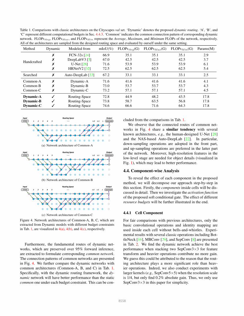
Table 1. Comparisons with classic architectures on the Cityscapes val set. ‘Dynamic’ denotes the proposed dynamic routing. ‘A’, ‘B’, and

‘C’ represent different computational budgets in Sec. 4.4.3. ‘Common’ indicates the common connection pattern of corresponding dynamic

network. FLOPsAvg , FLOPsMax, and FLOPsMin represent the Average, Maximum, and Minimum FLOPs of the network, respectively.

All of the architectures are sampled from the designed routing space and evaluated by ourself under the same setting.

Method Dynamic Modeled from mIoU(%) FLOPsAvg(G) FLOPsMax(G) FLOPsMin(G) Params(M)

Handcrafted

✗ FCN-32s [24] 66.9 35.1 35.1 35.1 2.9

✗ DeepLabV3 [5] 67.0 42.5 42.5 42.5 3.7

✗ U-Net [28] 71.6 53.9 53.9 53.9 6.1

✗ HRNetV2 [32] 72.5 62.5 62.5 62.5 5.4

Searched ✗ Auto-DeepLab [22] 67.2 33.1 33.1 33.1 2.5

Common-A ✗ Dynamic-A 71.6 41.6 41.6 41.6 4.1

Common-B ✗ Dynamic-B 73.0 53.7 53.7 53.7 4.3

Common-C ✗ Dynamic-C 73.2 57.1 57.1 57.1 4.5

Dynamic-A ✓ Routing-Space 72.8 44.9 48.2 43.5 17.8

Dynamic-B ✓ Routing-Space 73.8 58.7 63.5 56.8 17.8

Dynamic-C ✓ Routing-Space 74.6 66.6 71.6 64.3 17.8

…...…...

…...…...

…...…...

…...…...

…...…...

STEM

OutputInput

Upsample

Routing Space

1 2 3 4 5 …... L-2 L-1 L

4

8

6

2

le

STEM

OutputInput

Upsample

Routing Space

1 2 3 4 5 …... L-2 L-1 L

4

8

6

2

le

…...…...

(a) Network architecture of Common-A

…...…...

…...…...

…...…...

…...…...

STEM

OutputInput

Upsample

Routing Space

1 2 3 4 5 …... L-2 L-1 L

4

8

6

2

le

STEM

OutputInput

Upsample

Routing Space

1 2 3 4 5 …... L-2 L-1 L

4

8

6

2

le

(b) Network architecture of Common-B

…...…...

…...…...

…...…...

…...…...

…...…...

…...…...

STEM

OutputInput

Upsample

Routing Space

1 2 3 4 5 …... L-2 L-1 L

6

2

le

STEM

OutputInput

Upsample

Routing Space

1 2 3 4 5 …... L-2 L-1 L

6

2

le

(c) Network architecture of Common-C

Figure 4. Network architectures of Common-A, B, C, which are

extracted from Dynamic models with different budget constraints

in Tab. 1, are visualized in 4(a), 4(b), and 4(c), respectively.

Furthermore, the fundamental routes of dynamic net-

works, which are preserved over 95% forward inference,

are extracted to formulate corresponding common network.

The connection patterns of common networks are presented

in Fig. 4. We further compare the dynamic networks with

common architectures (Common-A, B, and C) in Tab. 1.

Specifically, with the dynamic routing framework, the dy-

namic network will have better performance than the static

common one under each budget constraint. This can be con-

cluded from the comparisons in Tab. 1.

We observe that the connected routes of common net-

works in Fig. 4 share a similar tendency with several

known architectures, e.g., the human-designed U-Net [28]

and the NAS-based Auto-DeepLab [22]. In particular,

down-sampling operations are adopted in the front part,

and up-sampling operations are preferred in the latter part

of the network. Moreover, high-resolution features in the

low-level stage are needed for object details (visualized in

Fig. 1), which may lead to better performance.

4.4. Component­wise Analysis

To reveal the effect of each component in the proposed

method, we will decompose our approach step-by-step in

this section. Firstly, the components inside cells will be dis-

cussed in detail. Then we investigate the activation function

of the proposed soft conditional gate. The effect of different

resource budgets will be further illustrated in the end.

4.4.1 Cell Component

For fair comparisons with previous architectures, only the

basic convolutional operations and identity mapping are

used inside each cell without bells-and-whistles. Experi-

mental results with several classic operations including Bot-

tleNeck [16], MBConv [29], and SepConv [8] are presented

in Tab. 2. We find the dynamic network achieve the best

performance when stacking two SepConv3×3 for feature

transform and heavier operations contribute no more gain.

We guess this could be attributed to the reason that the rout-

ing architecture plays a more significant role than heav-

ier operations. Indeed, we also conduct experiments with

larger kernels (e.g., SepConv5×5) when the resolution scale

is 1/4, but only find 0.2% absolute gain. Thus, we only use

SepConv3×3 in this paper for simplicity.

8558

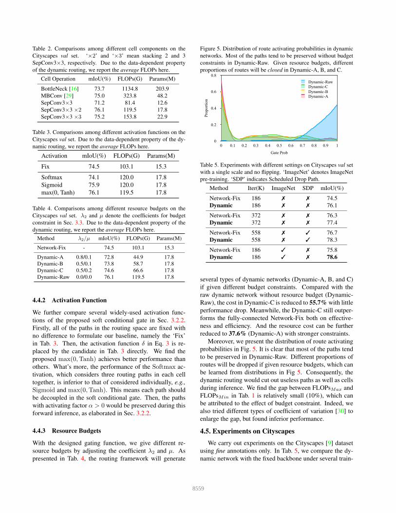
Table 2. Comparisons among different cell components on the

Cityscapes val set. ‘×2’ and ‘×3’ mean stacking 2 and 3

SepConv3×3, respectively. Due to the data-dependent property

of the dynamic routing, we report the average FLOPs here.

Cell Operation mIoU(%) FLOPs(G) Params(M)

BottleNeck [16] 73.7 1134.8 203.9

MBConv [29] 75.0 323.8 48.2

SepConv3×3 71.2 81.4 12.6

SepConv3×3 ×2 76.1 119.5 17.8

SepConv3×3 ×3 75.2 153.8 22.9

Table 3. Comparisons among different activation functions on the

Cityscapes val set. Due to the data-dependent property of the dy-

namic routing, we report the average FLOPs here.

Activation mIoU(%) FLOPs(G) Params(M)

Fix 74.5 103.1 15.3

Softmax 74.1 120.0 17.8

Sigmoid 75.9 120.0 17.8

max(0, Tanh) 76.1 119.5 17.8

Table 4. Comparisons among different resource budgets on the

Cityscapes val set. λ2 and µ denote the coefficients for budget

constraint in Sec. 3.3. Due to the data-dependent property of the

dynamic routing, we report the average FLOPs here.

Method λ2/µ mIoU(%) FLOPs(G) Params(M)

Network-Fix - 74.5 103.1 15.3

Dynamic-A 0.8/0.1 72.8 44.9 17.8

Dynamic-B 0.5/0.1 73.8 58.7 17.8

Dynamic-C 0.5/0.2 74.6 66.6 17.8

Dynamic-Raw 0.0/0.0 76.1 119.5 17.8

4.4.2 Activation Function

We further compare several widely-used activation func-

tions of the proposed soft conditional gate in Sec. 3.2.2.

Firstly, all of the paths in the routing space are fixed with

no difference to formulate our baseline, namely the ‘Fix’

in Tab. 3. Then, the activation function δ in Eq. 3 is re-

placed by the candidate in Tab. 3 directly. We find the

proposed max(0,Tanh) achieves better performance than

others. What’s more, the performance of the Softmax ac-

tivation, which considers three routing paths in each cell

together, is inferior to that of considered individually, e.g.,

Sigmoid and max(0,Tanh). This means each path should

be decoupled in the soft conditional gate. Then, the paths

with activating factor α > 0 would be preserved during this

forward inference, as elaborated in Sec. 3.2.2.

4.4.3 Resource Budgets

With the designed gating function, we give different re-

source budgets by adjusting the coefficient λ2 and µ. As

presented in Tab. 4, the routing framework will generate

Figure 5. Distribution of route activating probabilities in dynamic

networks. Most of the paths tend to be preserved without budget

constraints in Dynamic-Raw. Given resource budgets, different

proportions of routes will be closed in Dynamic-A, B, and C.

Pro

port

ion

0

0.2

0.4

0.6

0.8

Gate Prob

0 0.1 0.2 0.3 0.4 0.5 0.6 0.7 0.8 0.9 1

Dynamic-RawDynamic-C

Dynamic-BDynamic-A

Table 5. Experiments with different settings on Cityscapes val set

with a single scale and no flipping. ‘ImageNet’ denotes ImageNet

pre-training. ‘SDP’ indicates Scheduled Drop Path.

Method Iter(K) ImageNet SDP mIoU(%)

Network-Fix 186 ✗ ✗ 74.5

Dynamic 186 ✗ ✗ 76.1

Network-Fix 372 ✗ ✗ 76.3

Dynamic 372 ✗ ✗ 77.4

Network-Fix 558 ✗ ✓ 76.7

Dynamic 558 ✗ ✓ 78.3

Network-Fix 186 ✓ ✗ 75.8

Dynamic 186 ✓ ✗ 78.6

several types of dynamic networks (Dynamic-A, B, and C)

if given different budget constraints. Compared with the

raw dynamic network without resource budget (Dynamic-

Raw), the cost in Dynamic-C is reduced to 55.7% with little

performance drop. Meanwhile, the Dynamic-C still outper-

forms the fully-connected Network-Fix both on effective-

ness and efficiency. And the resource cost can be further

reduced to 37.6% (Dynamic-A) with stronger constraints.

Moreover, we present the distribution of route activating

probabilities in Fig. 5. It is clear that most of the paths tend

to be preserved in Dynamic-Raw. Different proportions of

routes will be dropped if given resource budgets, which can

be learned from distributions in Fig 5. Consequently, the

dynamic routing would cut out useless paths as well as cells

during inference. We find the gap between FLOPsMax and

FLOPsMin in Tab. 1 is relatively small (10%), which can

be attributed to the effect of budget constraint. Indeed, we

also tried different types of coefficient of variation [30] to

enlarge the gap, but found inferior performance.

4.5. Experiments on Cityscapes

We carry out experiments on the Cityscapes [9] dataset

using fine annotations only. In Tab. 5, we compare the dy-

namic network with the fixed backbone under several train-

8559

Table 6. Comparisons with previous works on the Cityscapes. mIoUtest and mIoUval denote performance on test set and val set respec-

tively. Multi-scale and flipping strategy are used in test set but dropped in val set. We report FLOPs with input size 1024× 2048.

Method Backbone mIoUtest(%) mIoUval(%) FLOPs(G)

BiSenet [40] ResNet-18 77.7 74.8 98.3†

DeepLabV3 [5] ResNet-101-ASPP - 78.5 1778.7

Semantic FPN [19] ResNet-101-FPN - 77.7 500.0

DeepLabV3+ [6] Xception-71-ASPP - 79.6 1551.1

PSPNet [43] ResNet-101-PSP 78.4 79.7 2017.6

Auto-DeepLab* [22] Searched-F20-ASPP 79.9 79.7 333.3

Auto-DeepLab* [22] Searched-F48-ASPP 80.4 80.3 695.0

Dynamic* Layer16 79.1 78.3 111.7

Dynamic Layer16 79.7 78.6 119.4

Dynamic Layer33 80.0 79.2 242.3

Dynamic Layer33-PSP 80.7 79.7 270.0

† estimated from corresponding settings* training from scratch

Table 7. Comparisons with previous works on the PASCAL VOC 2012. mIoUtest and mIoUval denote performance on test set and val set

respectively. Multi-scale and flipping strategy are used in test set but dropped in val set. We report FLOPs with input size 512× 512.

Method Backbone mIoUtest(%) mIoUval(%) FLOPs(G)

DeepLabV3 [5] MobileNet-ASPP - 75.3 14.3

DeepLabV3 [5] MobileNetV2-ASPP - 75.7 5.8

Auto-DeepLab [22] Searched-F20-ASPP 82.5 78.3 41.7†

Dynamic Layer16 82.8 78.6 14.9

Dynamic Layer33 84.0 79.0 30.8

† estimated from corresponding settings

ing settings on the val set. The proposed method achieves

consistent improvement in different situations. With the

Scheduled Drop Path [46, 22] and ImageNet [10] pre-

training, the performance of the dynamic network (L = 16)

can be further improved. Comparisons with several previ-

ous works are given in Tab. 6. With the similar resource

cost, the proposed dynamic network attains 78.6% mIoU

on the val set, which achieves a 3.8% absolute gain over

the well-designed BiSenet [40]. With the simple scale trans-

form modules without bells-and-whistles, the dynamic net-

work (L = 33) achieves comparable performance with the

state-of-the-art but consumes much fewer cost. Moreover,

in conjunction with the context capturing module (e.g., PSP

block), the proposed method has further improvements and

achieves 80.7% mIoU on the Cityscapes test set.

4.6. Experiments on PASCAL VOC

We further compare with similar methods (pre-trained

on the COCO [21] dataset), which focus on the architec-

ture design with comparable computational overhead, on

the PASCAL VOC 2012 [11] dataset. In particular, the

proposed approach surpasses Auto-DeepLab [22], which

would cost 3 GPU days for architecture searching, in both

accuracy and efficiency, as shown in Tab. 7. Compared with

the MobileNet-based DeepLabV3 [5], the dynamic network

still attains better performance with a similar resource cost.

5. Conclusion

In this work, we present the dynamic routing for seman-

tic segmentation. The key difference from prior works lies

in that we generate data-dependent forward paths according

to the scale distribution of each image. To this end, the soft

conditional gate is proposed to select scale transformation

routes in an end-to-end manner, which will learn to drop

useless operations for efficiency if given resource budgets.

Extensive ablation studies have been conducted to demon-

strate the superiority of the dynamic network over several

static architectures, which can be modeled in the designed

routing space. Experiments on Cityscapes and PASCAL

VOC 2012 prove the effectiveness of the proposed method,

which achieves comparable performance with state-of-the-

arts but consumes much fewer computational resources.

Acknowledgement

This work was supported by National Key Research and

Development Program of China 2018YFD0400902 and Na-

tional Natural Science Foundation of China 61573349.

8560

References

[1] Vijay Badrinarayanan, Alex Kendall, and Roberto Cipolla.

Segnet: A deep convolutional encoder-decoder architecture

for image segmentation. TPAMI, 2017. 1, 2

[2] Han Cai, Ligeng Zhu, and Song Han. Proxylessnas: Direct

neural architecture search on target task and hardware. In

ICLR, 2019. 2

[3] Liang-Chieh Chen, Maxwell Collins, Yukun Zhu, George

Papandreou, Barret Zoph, Florian Schroff, Hartwig Adam,

and Jon Shlens. Searching for efficient multi-scale architec-

tures for dense image prediction. In NeurIPS, 2018. 1, 2

[4] Liang-Chieh Chen, George Papandreou, Iasonas Kokkinos,

Kevin Murphy, and Alan L Yuille. Deeplab: Semantic image

segmentation with deep convolutional nets, atrous convolu-

tion, and fully connected crfs. TPAMI, 2017. 2

[5] Liang-Chieh Chen, George Papandreou, Florian Schroff, and

Hartwig Adam. Rethinking atrous convolution for semantic

image segmentation. arXiv:1706.05587, 2017. 2, 4, 5, 6, 8

[6] Liang-Chieh Chen, Yukun Zhu, George Papandreou, Florian

Schroff, and Hartwig Adam. Encoder-decoder with atrous

separable convolution for semantic image segmentation. In

ECCV, 2018. 1, 2, 8

[7] Xin Chen, Lingxi Xie, Jun Wu, and Qi Tian. Progressive dif-

ferentiable architecture search: Bridging the depth gap be-

tween search and evaluation. In ICCV, 2019. 2

[8] Francois Chollet. Xception: Deep learning with depthwise

separable convolutions. In CVPR, 2017. 6

[9] Marius Cordts, Mohamed Omran, Sebastian Ramos, Timo

Rehfeld, Markus Enzweiler, Rodrigo Benenson, Uwe

Franke, Stefan Roth, and Bernt Schiele. The cityscapes

dataset for semantic urban scene understanding. In CVPR,

2016. 2, 5, 7

[10] Jia Deng, Wei Dong, Richard Socher, Li-Jia Li, Kai Li,

and Li Fei-Fei. Imagenet: A large-scale hierarchical image

database. In CVPR, 2009. 5, 8

[11] Mark Everingham, Luc Van Gool, Christopher KI Williams,

John Winn, and Andrew Zisserman. The pascal visual object

classes (voc) challenge. IJCV, 2010. 2, 5, 8

[12] Jun Fu, Jing Liu, Haijie Tian, Yong Li, Yongjun Bao, Zhiwei

Fang, and Hanqing Lu. Dual attention network for scene

segmentation. In CVPR, 2019. 2

[13] Zichao Guo, Xiangyu Zhang, Haoyuan Mu, Wen Heng,

Zechun Liu, Yichen Wei, and Jian Sun. Single path

one-shot neural architecture search with uniform sampling.

arXiv:1904.00420, 2019. 2

[14] Bharath Hariharan, Pablo Arbelaez, Lubomir Bourdev,

Subhransu Maji, and Jitendra Malik. Semantic contours from

inverse detectors. In ICCV, 2011. 5

[15] Kaiming He, Xiangyu Zhang, Shaoqing Ren, and Jian Sun.

Delving deep into rectifiers: Surpassing human-level perfor-

mance on imagenet classification. In ICCV, 2015. 5

[16] Kaiming He, Xiangyu Zhang, Shaoqing Ren, and Jian Sun.

Deep residual learning for image recognition. In CVPR,

2016. 5, 6, 7

[17] Gao Huang, Danlu Chen, Tianhong Li, Felix Wu, Laurens

van der Maaten, and Kilian Q Weinberger. Multi-scale dense

networks for resource efficient image classification. In ICLR,

2018. 2

[18] Zilong Huang, Xinggang Wang, Lichao Huang, Chang

Huang, Yunchao Wei, and Wenyu Liu. Ccnet: Criss-cross

attention for semantic segmentation. In ICCV, 2019. 2

[19] Alexander Kirillov, Ross Girshick, Kaiming He, and Piotr

Dollar. Panoptic feature pyramid networks. In CVPR, 2019.

1, 8

[20] Ji Lin, Yongming Rao, Jiwen Lu, and Jie Zhou. Runtime

neural pruning. In NeurIPS, 2017. 2

[21] Tsung-Yi Lin, Michael Maire, Serge Belongie, James Hays,

Pietro Perona, Deva Ramanan, Piotr Dollar, and C Lawrence

Zitnick. Microsoft coco: Common objects in context. In

ECCV, 2014. 8

[22] Chenxi Liu, Liang-Chieh Chen, Florian Schroff, Hartwig

Adam, Wei Hua, Alan L Yuille, and Li Fei-Fei. Auto-

deeplab: Hierarchical neural architecture search for semantic

image segmentation. In CVPR, 2019. 1, 2, 3, 4, 5, 6, 8

[23] Hanxiao Liu, Karen Simonyan, and Yiming Yang. Darts:

Differentiable architecture search. In ICLR, 2019. 2, 3, 4

[24] Jonathan Long, Evan Shelhamer, and Trevor Darrell. Fully

convolutional networks for semantic segmentation. In

CVPR, 2015. 1, 2, 4, 5, 6

[25] Vladimir Nekrasov, Hao Chen, Chunhua Shen, and Ian Reid.

Fast neural architecture search of compact semantic segmen-

tation models via auxiliary cells. In CVPR, 2019. 1, 2

[26] Hyeonwoo Noh, Seunghoon Hong, and Bohyung Han.

Learning deconvolution network for semantic segmentation.

In ICCV, 2015. 2

[27] Hieu Pham, Melody Y Guan, Barret Zoph, Quoc V Le, and

Jeff Dean. Efficient neural architecture search via parameter

sharing. In ICML, 2018. 2

[28] Olaf Ronneberger, Philipp Fischer, and Thomas Brox. U-net:

Convolutional networks for biomedical image segmentation.

In MICCAI, 2015. 1, 2, 4, 5, 6

[29] Mark Sandler, Andrew Howard, Menglong Zhu, Andrey Zh-

moginov, and Liang-Chieh Chen. Mobilenetv2: Inverted

residuals and linear bottlenecks. In CVPR, 2018. 6, 7

[30] Noam Shazeer, Azalia Mirhoseini, Krzysztof Maziarz, Andy

Davis, Quoc Le, Geoffrey Hinton, and Jeff Dean. Outra-

geously large neural networks: The sparsely-gated mixture-

of-experts layer. In ICLR, 2017. 7

[31] Lin Song, Yanwei Li, Zeming Li, Gang Yu, Hongbin Sun,

Jian Sun, and Nanning Zheng. Learnable tree filter for

structure-preserving feature transform. In NeurIPS, 2019.

1, 2, 5

[32] Ke Sun, Yang Zhao, Borui Jiang, Tianheng Cheng, Bin Xiao,

Dong Liu, Yadong Mu, Xinggang Wang, Wenyu Liu, and

Jingdong Wang. High-resolution representations for labeling

pixels and regions. arXiv:1904.04514, 2019. 1, 4, 5, 6

[33] Ravi Teja Mullapudi, William R Mark, Noam Shazeer, and

Kayvon Fatahalian. Hydranets: Specialized dynamic archi-

tectures for efficient inference. In CVPR, 2018. 2

[34] Tom Veniat and Ludovic Denoyer. Learning time/memory-

efficient deep architectures with budgeted super networks. In

CVPR, 2018. 4

8561

[35] Xiaolong Wang, Ross Girshick, Abhinav Gupta, and Kaim-

ing He. Non-local neural networks. In CVPR, 2018. 1

[36] Xin Wang, Fisher Yu, Zi-Yi Dou, Trevor Darrell, and

Joseph E Gonzalez. Skipnet: Learning dynamic routing in

convolutional networks. In ECCV, 2018. 2, 4

[37] Bichen Wu, Xiaoliang Dai, Peizhao Zhang, Yanghan Wang,

Fei Sun, Yiming Wu, Yuandong Tian, Peter Vajda, Yangqing

Jia, and Kurt Keutzer. Fbnet: Hardware-aware efficient con-

vnet design via differentiable neural architecture search. In

CVPR, 2019. 4

[38] Zuxuan Wu, Tushar Nagarajan, Abhishek Kumar, Steven

Rennie, Larry S Davis, Kristen Grauman, and Rogerio Feris.

Blockdrop: Dynamic inference paths in residual networks.

In CVPR, 2018. 2, 4

[39] Zhonghui You, Kun Yan, Jinmian Ye, Meng Ma, and Ping

Wang. Gate decorator: Global filter pruning method for ac-

celerating deep convolutional neural networks. In NeurIPS,

2019. 2

[40] Changqian Yu, Jingbo Wang, Chao Peng, Changxin Gao,

Gang Yu, and Nong Sang. Bisenet: Bilateral segmenta-

tion network for real-time semantic segmentation. In ECCV,

2018. 2, 5, 8

[41] Changqian Yu, Jingbo Wang, Chao Peng, Changxin Gao,

Gang Yu, and Nong Sang. Learning a discriminative feature

network for semantic segmentation. In CVPR, 2018. 2

[42] Hengshuang Zhao, Xiaojuan Qi, Xiaoyong Shen, Jianping

Shi, and Jiaya Jia. Icnet for real-time semantic segmentation

on high-resolution images. In ECCV, 2018. 2

[43] Hengshuang Zhao, Jianping Shi, Xiaojuan Qi, Xiaogang

Wang, and Jiaya Jia. Pyramid scene parsing network. In

CVPR, 2017. 1, 2, 8

[44] Hengshuang Zhao, Yi Zhang, Shu Liu, Jianping Shi, Chen

Change Loy, Dahua Lin, and Jiaya Jia. Psanet: Point-wise

spatial attention network for scene parsing. In ECCV, 2018.

1, 2

[45] Barret Zoph and Quoc V Le. Neural architecture search with

reinforcement learning. In ICLR, 2017. 2

[46] Barret Zoph, Vijay Vasudevan, Jonathon Shlens, and Quoc V

Le. Learning transferable architectures for scalable image

recognition. In CVPR, 2018. 3, 8

8562