Embed Size (px)
Citation preview
Learning GAMS forPower Generation Operation and Control
Luigi Vanfretti
Rensselaer Polytechnic Institute
April 4, 2006.
Luigi Vanfretti, RPI – p.1/30
Outlook of this talk
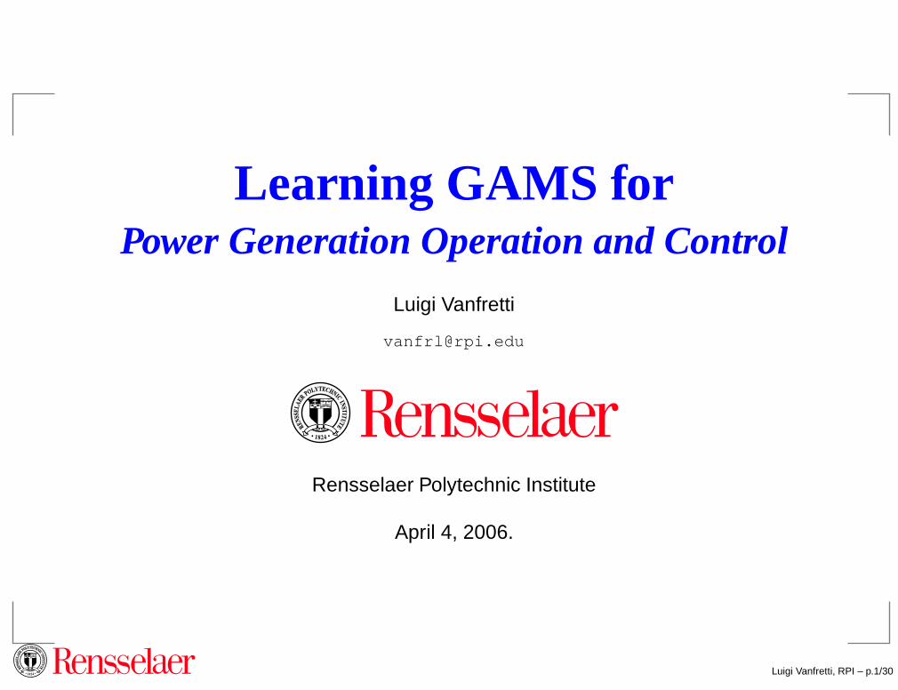
What are we going to talk about?
About GAMSWhat is GAMS?Using GAMS for POG&CDownloading GAMSSome Features of GAMSParts of a GAMS Model (Program)
Some problems of POG&C that can be solved withGAMS
Economic DispatchUnit Commitment
Luigi Vanfretti, RPI – p.2/30
What is GAMS?
GAMS (Generalized Algebra Modelling System) is acomputer enviorment that can easily be used to modeland solve optimization problems. GAMS is speciallydesign for linear, nonlinear and mixed integeroptimization.
An interesting fact is that GAMS was developed "out of the
frustaging experiences of an economic modeling group at the World Bank...
The programmers in the group wrote FORTRAN programs to prepare each
model fro solution; the work was dull but demanding, and errors were easy to
make and hard to find" [4]. .
Even though it is required some effor to become familiarwith GAMS, we will se that this is a very small cost to payto have a comprehensive and very powerfull tool to solvepower systems optimization problems.
Luigi Vanfretti, RPI – p.3/30
Using GAMS for POG&C
In EPOW-6840 Power Generation Operation andControl, all the topics covered involve the solution of anoptimization problem.
There are many available tools that can solve powersystem optimization problems, but most of them are notsuitable for learning the basic concepts since themodelling details are transparent to the user.
Thus, GAMS presents an adequate tool to solve theoptimization problems that we deal in PGO&C.
The power systems problems that we analyze here are:Economic Dispatch (lossless and with losses) and theUnit Commitment (with different constraints), bothpresented in [1], .
For those interested, there are many other examplespresented in [1], [4], [2], [3] and [8]. Luigi Vanfretti, RPI – p.4/30

Downloading GAMS
A free demo of the current distribution, as well as pastdistributions, is available at http://www.gams.com/
Without a license, the GAMS distribution has thefollowing limitations:
Model limits:Up to 200 constraintsUp to 300 variablesUp to 2000 nonzero elements (1000 nonlinear).
Up to 30 discrete variables.
Solver (Global) limits:Up to 10 constranints.
Up to 10 variables.
Note that this limitations are not a problem foreducational purposes since we are not solving largescale networks.
Luigi Vanfretti, RPI – p.5/30
GAMS Features
The most important features of GAMS are:
Capability to solve from small scale to large scaleproblems with small code by means of the use of indexto write blocks of similar constraints from only oneconstraint.
The model is independent from the solution method, andit can be solved by different solutions methos by onlychanging the solver.
The translation from the mathematical model to GAMS isalmost transparent since GAMS has been built toresemble mathematical programming models.
GAMS also uses common english words, thus is easy tounderstand it’s statements.
Luigi Vanfretti, RPI – p.6/30

Parts of a GAMS Model
The parts of a GAMS Model or Program are defined in thetable below:
COMMAND PURPOSE
SET Used to indicate the name of the indices
SCALAR Used to declare scalars
PARAMETER Used to declare vectors
TABLE Declare and assign the values of an array
VARIABLE Declare variables, assign type and bounds
EQUATION Function to be optimized and it’s constraints
MODEL Give a name to the model, and list the related constraints
SOLVE Indicate what solver to use
DISPLAY Indicate what you would like to display as output
Table 1: Main Commands of GAMS
We will now define each of this parts with the use of a eco-nomic dispatch example presented in [1].
Luigi Vanfretti, RPI – p.7/30
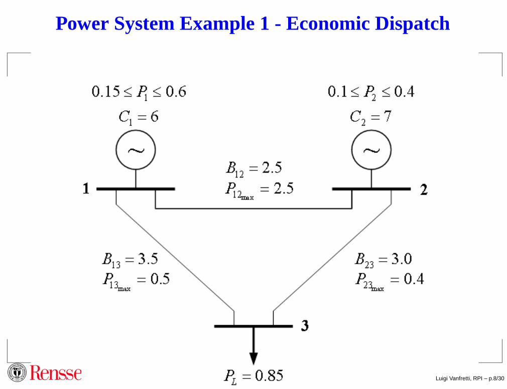
Power System Example 1 - Economic Dispatch
Luigi Vanfretti, RPI – p.8/30
Sets
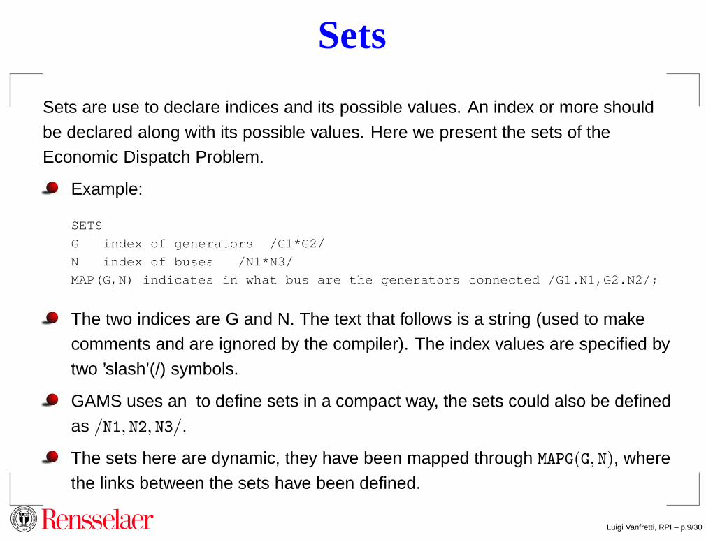
Sets are use to declare indices and its possible values. An index or more should
be declared along with its possible values. Here we present the sets of theEconomic Dispatch Problem.
Example:
SETS
G index of generators /G1*G2/
N index of buses /N1*N3/
MAP(G,N) indicates in what bus are the generators connected /G1.N1,G2.N2/;
The two indices are G and N. The text that follows is a string (used to makecomments and are ignored by the compiler). The index values are specified by
two ’slash’(/) symbols.
GAMS uses an to define sets in a compact way, the sets could also be defined
as /N1, N2, N3/.
The sets here are dynamic, they have been mapped through MAPG(G, N), where
the links between the sets have been defined.
Luigi Vanfretti, RPI – p.9/30
Scalars
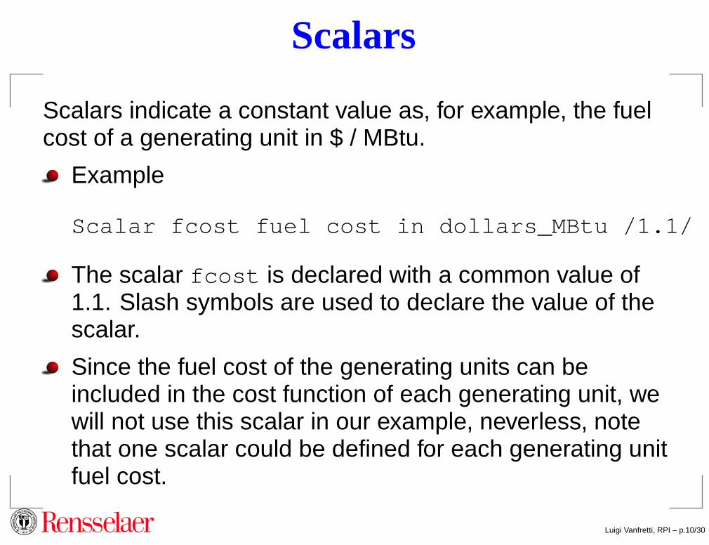
Scalars indicate a constant value as, for example, the fuelcost of a generating unit in $ / MBtu.
Example
Scalar fcost fuel cost in dollars_MBtu /1.1/
The scalar fcost is declared with a common value of1.1. Slash symbols are used to declare the value of thescalar.
Since the fuel cost of the generating units can beincluded in the cost function of each generating unit, wewill not use this scalar in our example, neverless, notethat one scalar could be defined for each generating unitfuel cost.
Luigi Vanfretti, RPI – p.10/30
Parameters
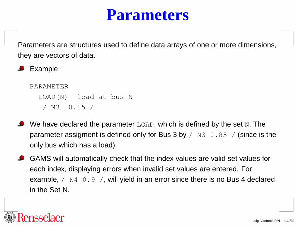
Parameters are structures used to define data arrays of one or more dimensions,
they are vectors of data.
Example
PARAMETER
LOAD(N) load at bus N
/ N3 0.85 /
We have declared the parameter LOAD, which is defined by the set N. Theparameter assigment is defined only for Bus 3 by / N3 0.85 / (since is the
only bus which has a load).
GAMS will automatically check that the index values are valid set values for
each index, displaying errors when invalid set values are entered. Forexample, / N4 0.9 / , will yield in an error since there is no Bus 4 declared
in the Set N.
Luigi Vanfretti, RPI – p.11/30
Tables - I
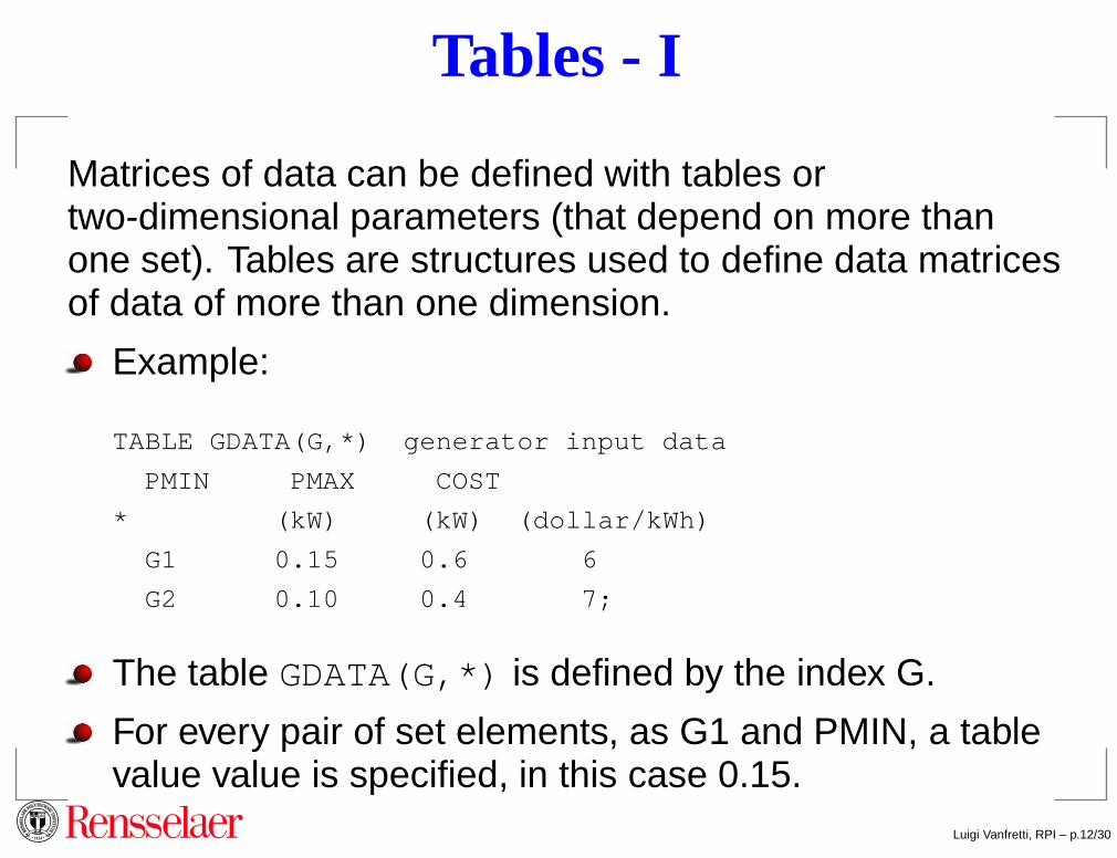
Matrices of data can be defined with tables ortwo-dimensional parameters (that depend on more thanone set). Tables are structures used to define data matricesof data of more than one dimension.
Example:
TABLE GDATA(G,*) generator input data
PMIN PMAX COST
* (kW) (kW) (dollar/kWh)
G1 0.15 0.6 6
G2 0.10 0.4 7;
The table GDATA(G,*) is defined by the index G.
For every pair of set elements, as G1 and PMIN, a tablevalue value is specified, in this case 0.15.
Luigi Vanfretti, RPI – p.12/30
Tables - II
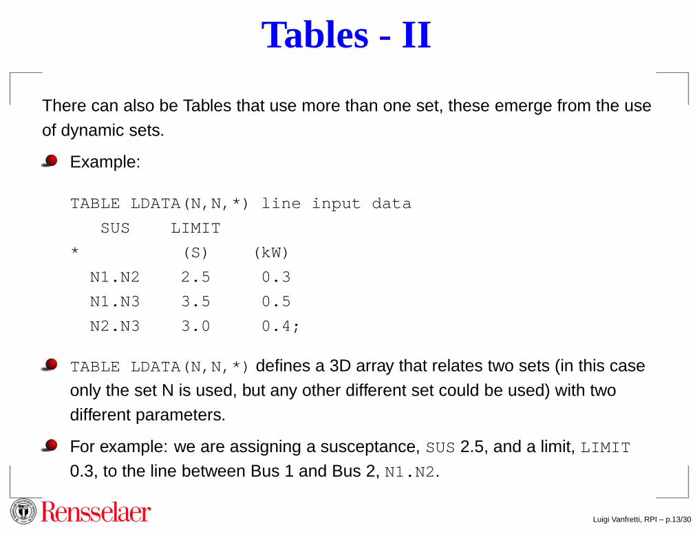
There can also be Tables that use more than one set, these emerge from the use
of dynamic sets.
Example:
TABLE LDATA(N,N,*) line input data
SUS LIMIT
* (S) (kW)
N1.N2 2.5 0.3
N1.N3 3.5 0.5
N2.N3 3.0 0.4;
TABLE LDATA(N,N,*) defines a 3D array that relates two sets (in this case
only the set N is used, but any other different set could be used) with twodifferent parameters.
For example: we are assigning a susceptance, SUS2.5, and a limit, LIMIT
0.3, to the line between Bus 1 and Bus 2, N1.N2 .
Luigi Vanfretti, RPI – p.13/30
Variables - I
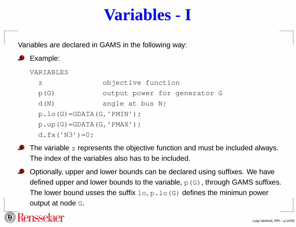
Variables are declared in GAMS in the following way:
Example:
VARIABLES
z objective function
p(G) output power for generator G
d(N) angle at bus N;
p.lo(G)=GDATA(G,’PMIN’);
p.up(G)=GDATA(G,’PMAX’);
d.fx(’N3’)=0;
The variable z represents the objective function and must be included always.
The index of the variables also has to be included.
Optionally, upper and lower bounds can be declared using suffixes. We havedefined upper and lower bounds to the variable, p(G) , through GAMS suffixes.
The lower bound usses the suffix lo , p.lo(G) defines the minimun poweroutput at node G.
Luigi Vanfretti, RPI – p.14/30
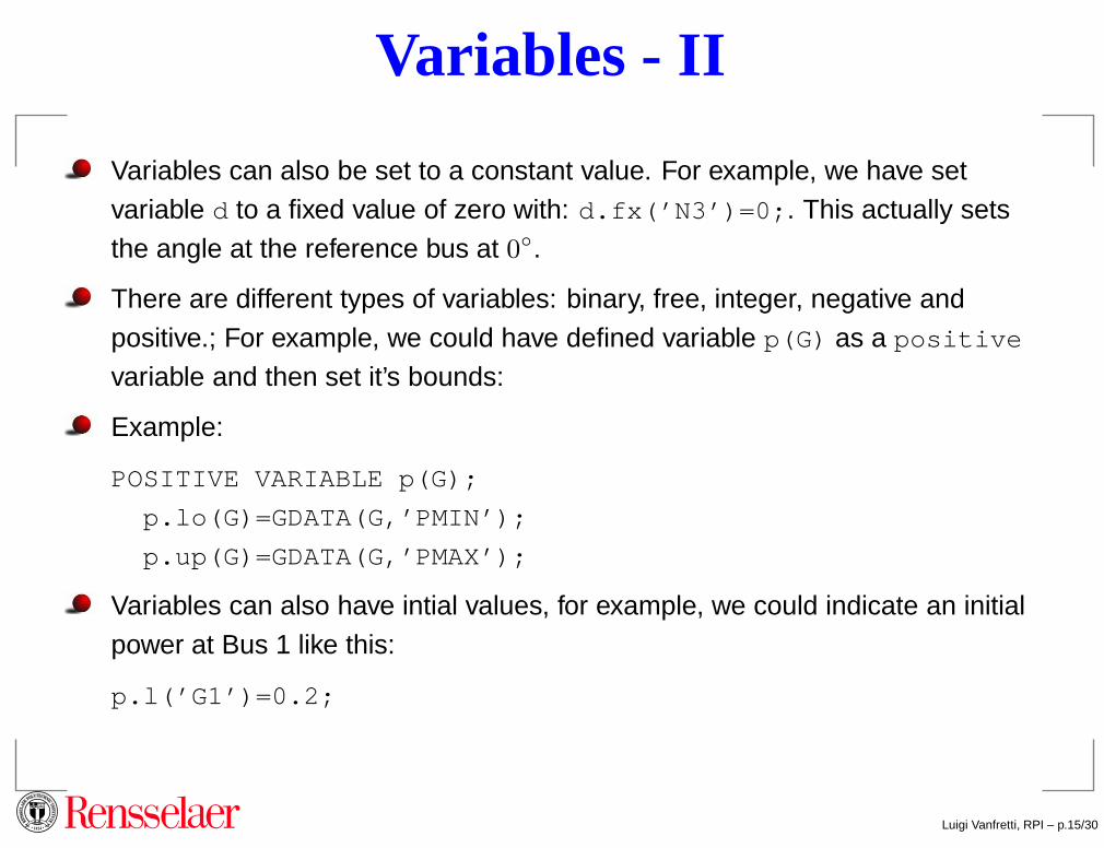
Variables - II
Variables can also be set to a constant value. For example, we have setvariable d to a fixed value of zero with: d.fx(’N3’)=0; . This actually sets
the angle at the reference bus at 0◦.
There are different types of variables: binary, free, integer, negative and
positive.; For example, we could have defined variable p(G) as a positive
variable and then set it’s bounds:
Example:
POSITIVE VARIABLE p(G);
p.lo(G)=GDATA(G,’PMIN’);
p.up(G)=GDATA(G,’PMAX’);
Variables can also have intial values, for example, we could indicate an initial
power at Bus 1 like this:
p.l(’G1’)=0.2;
Luigi Vanfretti, RPI – p.15/30
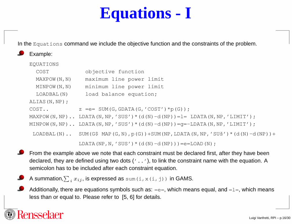
Equations - I
In the Equations command we include the objective function and the constraints of the problem.
Example:
EQUATIONS
COST objective function
MAXPOW(N,N) maximum line power limit
MINPOW(N,N) minimum line power limit
LOADBAL(N) load balance equation;
ALIAS(N,NP);
COST.. z =e= SUM(G,GDATA(G,’COST’)*p(G));
MAXPOW(N,NP).. LDATA(N,NP,’SUS’)*(d(N)-d(NP))=l= LDAT A(N,NP,’LIMIT’);
MINPOW(N,NP).. LDATA(N,NP,’SUS’)*(d(N)-d(NP))=g=-LDA TA(N,NP,’LIMIT’);
LOADBAL(N).. SUM(G$ MAP(G,N),p(G))+SUM(NP,LDATA(N,NP, ’SUš’)*(d(N)-d(NP))+
LDATA(NP,N,’SUS’)*(d(N)-d(NP)))=e=LOAD(N);
From the example above we note that each constraint must be declared first, after they have beendeclared, they are defined using two dots (’..’ ), to link the constraint name with the equation. Asemicolon has to be included after each constraint equation.
A summation,∑
ixij , is expressed as sum(i,x(i,j)) in GAMS.
Additionally, there are equations symbols such as: =e=, which means equal, and =l= , which meansless than or equal to. Please refer to [5, 6] for details.
Luigi Vanfretti, RPI – p.16/30
Equations - II
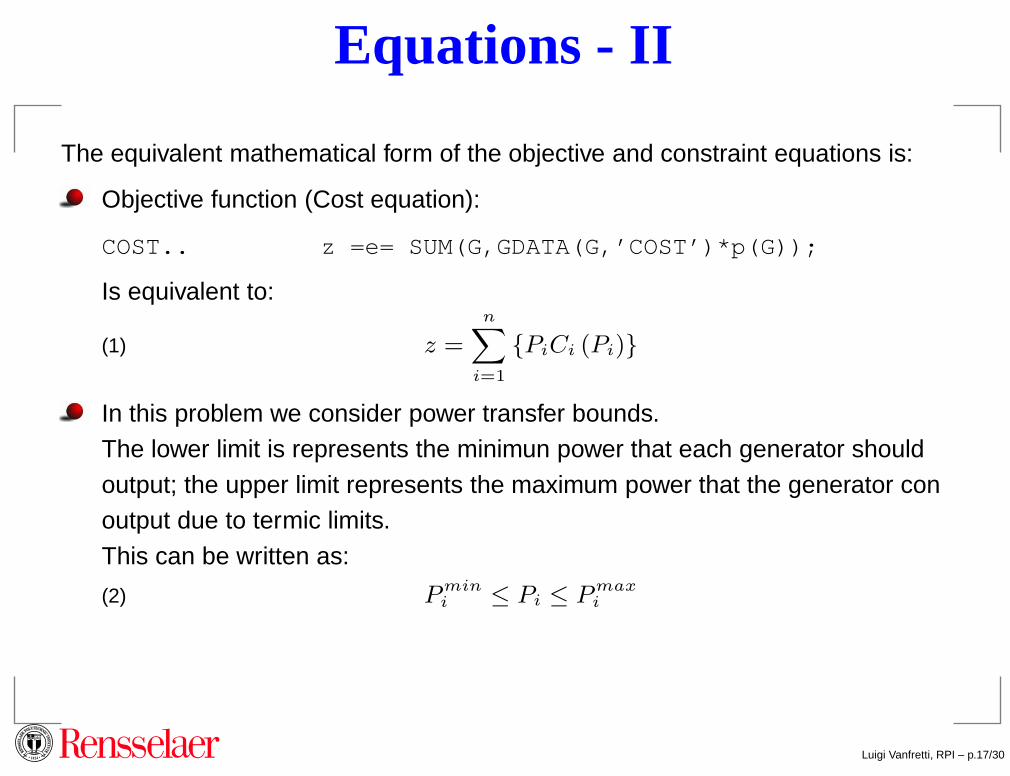
The equivalent mathematical form of the objective and constraint equations is:
Objective function (Cost equation):
COST.. z =e= SUM(G,GDATA(G,’COST’)*p(G));
Is equivalent to:
z =
n∑
i=1
{PiCi (Pi)}(1)
In this problem we consider power transfer bounds.The lower limit is represents the minimun power that each generator should
output; the upper limit represents the maximum power that the generator conoutput due to termic limits.
This can be written as:
P min
i ≤ Pi ≤ P max
i(2)
Luigi Vanfretti, RPI – p.17/30

Equations - III
The power transmitted in a transmission line is limited by thermal and stability considerations (angle).The power transmitted from Bus i to Bus j through the line i − j is:
Bij (δi − δj)(3)
Considering equations (??) and (??) we have the equation:
Pmin
i ≤ Bij (δi − δj) ≤ Pmax
i(4)
Equation (??) translates in the GAMS constraint equations:
MAXPOW(N,NP).. LDATA(N,NP,’SUS’)*(d(N)-d(NP))=l= LDAT A(N,NP,’LIMIT’);
MINPOW(N,NP).. LDATA(N,NP,’SUS’)*(d(N)-d(NP))=g=-LDA TA(N,NP,’LIMIT’);
The Power Balance equation is given by:
Pi = Di −∑
Bij (δi − δj)(5)
Which translates to: LOADBAL(N).. SUM(G$
MAP(G,N),p(G))+SUM(NP,LDATA(N,NP,’SUS’)*(d(N)-d(NP) )+
LDATA(NP,N,’SUS’)*(d(N)-d(NP)))=e=LOAD(N);
The term∑
Bij (δi − δj) implicitly considers losses (but as a constrain, they are not optimized).
Luigi Vanfretti, RPI – p.18/30
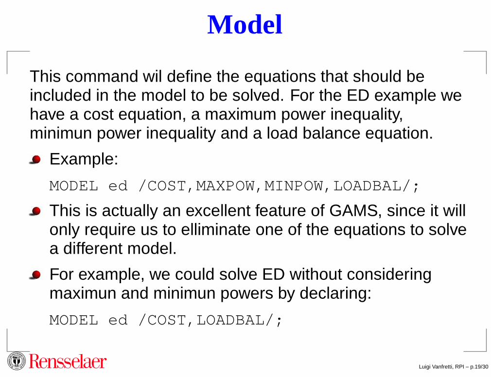
Model
This command wil define the equations that should beincluded in the model to be solved. For the ED example wehave a cost equation, a maximum power inequality,minimun power inequality and a load balance equation.
Example:
MODEL ed /COST,MAXPOW,MINPOW,LOADBAL/;
This is actually an excellent feature of GAMS, since it willonly require us to elliminate one of the equations to solvea different model.
For example, we could solve ED without consideringmaximun and minimun powers by declaring:
MODEL ed /COST,LOADBAL/;
Luigi Vanfretti, RPI – p.19/30
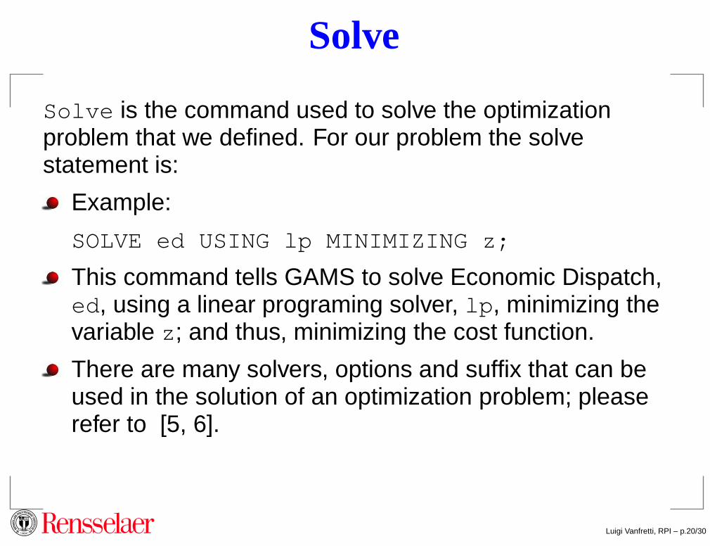
Solve
Solve is the command used to solve the optimizationproblem that we defined. For our problem the solvestatement is:
Example:
SOLVE ed USING lp MINIMIZING z;
This command tells GAMS to solve Economic Dispatch,ed , using a linear programing solver, lp , minimizing thevariable z ; and thus, minimizing the cost function.
There are many solvers, options and suffix that can beused in the solution of an optimization problem; pleaserefer to [5, 6].
Luigi Vanfretti, RPI – p.20/30
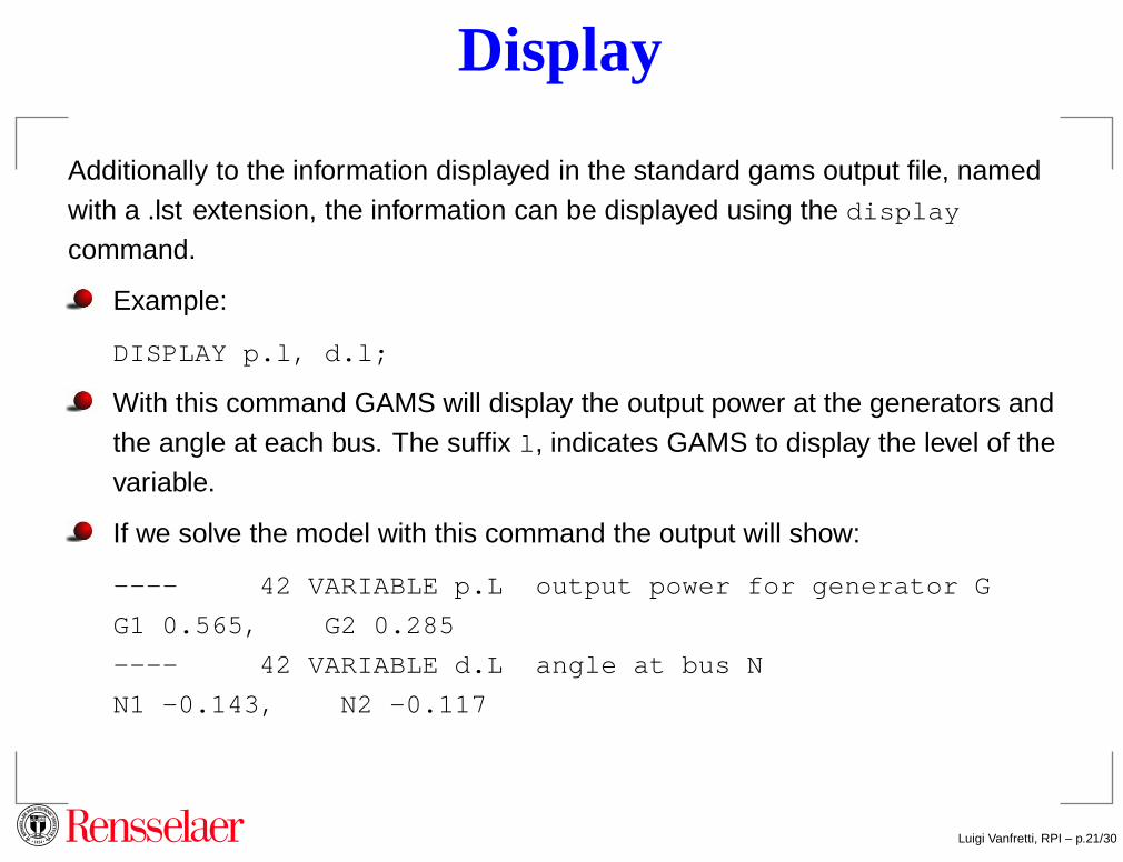
Display
Additionally to the information displayed in the standard gams output file, named
with a .lst extension, the information can be displayed using the display
command.
Example:
DISPLAY p.l, d.l;
With this command GAMS will display the output power at the generators and
the angle at each bus. The suffix l , indicates GAMS to display the level of thevariable.
If we solve the model with this command the output will show:
---- 42 VARIABLE p.L output power for generator G
G1 0.565, G2 0.285
---- 42 VARIABLE d.L angle at bus N
N1 -0.143, N2 -0.117
Luigi Vanfretti, RPI – p.21/30
Power System Example 2 - Unit Commitment
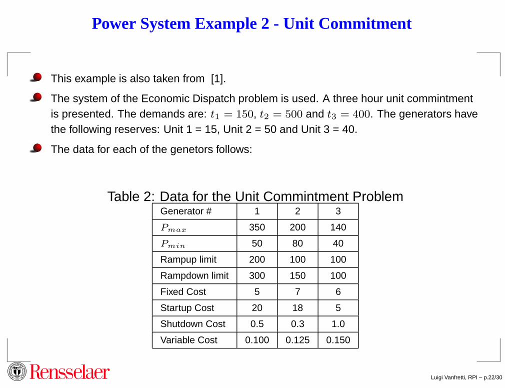
This example is also taken from [1].
The system of the Economic Dispatch problem is used. A three hour unit commintmentis presented. The demands are: t1 = 150, t2 = 500 and t3 = 400. The generators havethe following reserves: Unit 1 = 15, Unit 2 = 50 and Unit 3 = 40.
The data for each of the genetors follows:
Table 2: Data for the Unit Commintment ProblemGenerator # 1 2 3
Pmax 350 200 140
Pmin 50 80 40
Rampup limit 200 100 100
Rampdown limit 300 150 100
Fixed Cost 5 7 6
Startup Cost 20 18 5
Shutdown Cost 0.5 0.3 1.0
Variable Cost 0.100 0.125 0.150
Luigi Vanfretti, RPI – p.22/30

Power System Example 2 - Unit Commitment
SETS:
SETS
K index of periods of time /1*4/
J index of generators /1*3/
TABLES:
TABLE GDATA(J,*) generator input data
PMIN PMAX T S A B C E
* Ramp Ramp Fixed Variable Start Shutdown
* Down Up Cost Cost UP Cost
* Limit Limit Cost
* (kW) (kW) (kW/h) (kW/h) (E) (E) (E) (E/kWh)
1 50 350 300 200 5 20 0.5 0.100
2 80 200 150 100 7 18 0.3 0.125
3 40 140 100 100 6 5 1.0 0.150;
TABLE PDATA(K,*) data per period
D R
* Load Reserve
* (kW) (kW)
2 150 15
3 500 50
4 400 40;Luigi Vanfretti, RPI – p.23/30
Power System Example 2 - Unit Commitment
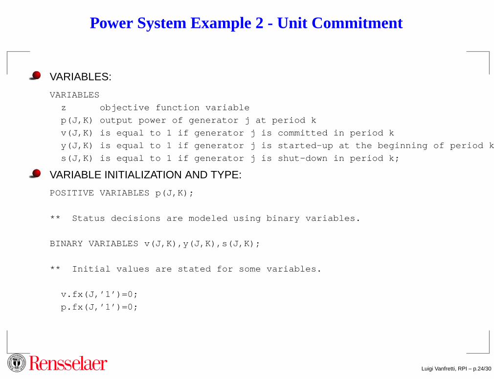
VARIABLES:
VARIABLES
z objective function variable
p(J,K) output power of generator j at period k
v(J,K) is equal to 1 if generator j is committed in period k
y(J,K) is equal to 1 if generator j is started-up at the beginn ing of period k
s(J,K) is equal to 1 if generator j is shut-down in period k;
VARIABLE INITIALIZATION AND TYPE:
POSITIVE VARIABLES p(J,K);
** Status decisions are modeled using binary variables.
BINARY VARIABLES v(J,K),y(J,K),s(J,K);
** Initial values are stated for some variables.
v.fx(J,’1’)=0;
p.fx(J,’1’)=0;
Luigi Vanfretti, RPI – p.24/30
Power System Example 2 - Unit Commitment
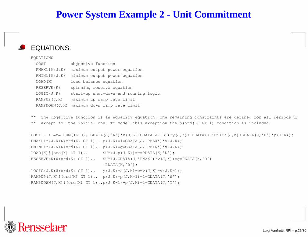
EQUATIONS:EQUATIONS
COST objective function
PMAXLIM(J,K) maximum output power equation
PMINLIM(J,K) minimum output power equation
LOAD(K) load balance equation
RESERVE(K) spinning reserve equation
LOGIC(J,K) start-up shut-down and running logic
RAMPUP(J,K) maximum up ramp rate limit
RAMPDOWN(J,K) maximum down ramp rate limit;
** The objective function is an equality equation. The remai ning constraints are defined for all periods K,
** except for the initial one. To model this exception the $(o rd(K) GT 1) condition is included.
COST.. z =e= SUM((K,J), GDATA(J,’A’)*v(J,K)+GDATA(J,’B’ )*y(J,K)+ GDATA(J,’C’)*s(J,K)+GDATA(J,’D’)*p(J,K));
PMAXLIM(J,K)$(ord(K) GT 1).. p(J,K)=l=GDATA(J,’PMAX’)* v(J,K);
PMINLIM(J,K)$(ord(K) GT 1).. p(J,K)=g=GDATA(J,’PMIN’)* v(J,K);
LOAD(K)$(ord(K) GT 1).. SUM(J,p(J,K))=e=PDATA(K,’D’);
RESERVE(K)$(ord(K) GT 1).. SUM(J,GDATA(J,’PMAX’)*v(J,K ))=g=PDATA(K,’D’)
+PDATA(K,’R’);
LOGIC(J,K)$(ord(K) GT 1).. y(J,K)-s(J,K)=e=v(J,K)-v(J, K-1);
RAMPUP(J,K)$(ord(K) GT 1).. p(J,K)-p(J,K-1)=l=GDATA(J, ’S’);
RAMPDOWN(J,K)$(ord(K) GT 1)..p(J,K-1)-p(J,K)=l=GDATA( J,’T’);
Luigi Vanfretti, RPI – p.25/30
Power System Example 2 - Unit Commitment
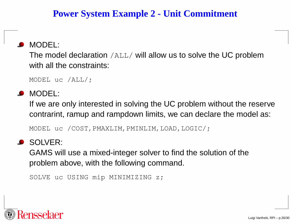
MODEL:The model declaration /ALL/ will allow us to solve the UC problemwith all the constraints:
MODEL uc /ALL/;
MODEL:If we are only interested in solving the UC problem without the reservecontrarint, ramup and rampdown limits, we can declare the model as:
MODEL uc /COST,PMAXLIM,PMINLIM,LOAD,LOGIC/;
SOLVER:GAMS will use a mixed-integer solver to find the solution of theproblem above, with the following command.
SOLVE uc USING mip MINIMIZING z;
Luigi Vanfretti, RPI – p.26/30
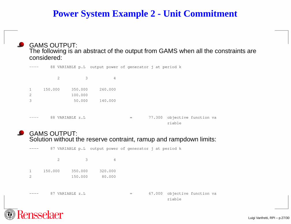
Power System Example 2 - Unit Commitment
GAMS OUTPUT:The following is an abstract of the output from GAMS when all the constraints areconsidered:---- 88 VARIABLE p.L output power of generator j at period k
2 3 4
1 150.000 350.000 260.000
2 100.000
3 50.000 140.000
---- 88 VARIABLE z.L = 77.300 objective function va
riable
GAMS OUTPUT:Solution without the reserve contraint, ramup and rampdown limits:---- 87 VARIABLE p.L output power of generator j at period k
2 3 4
1 150.000 350.000 320.000
2 150.000 80.000
---- 87 VARIABLE z.L = 67.000 objective function va
riable
Luigi Vanfretti, RPI – p.27/30
Thank you for your attention!
The files used in this presentation are online at:http://www.rpi.edu/~vanfrl/pogc.html
Luigi Vanfretti, RPI – p.28/30
References[1] E. Castillo, A. J. Conejo, P. Pedregal, R. García and N. Alguacil,
Building and Solving Mathematical Programming Models inEngineering and Science, John Wiley & Sons, 2002. Spanishversion available free at:http://departamentos.unican.es/macc/personal/
profesores/castillo/Libro.htm
[2] J. Restrepo, Power Applied GAMS Tutorial, Power EngineeringResearch Laboratory, McGill University.
[3] J. Restrepo, Introduction to GAMS, Power Engineering ResearchLaboratory, McGill University.
[4] D. Chattopadhyay, "Application of General Algebraic ModelingSystem to Power System Optimization," IEEE Transactions onPower Systems, vol. 14, no. 1, February 1999, pp. 15 - 22.
Luigi Vanfretti, RPI – p.29/30
References[5] R. E. Rosenthal. GAMS - A User’s Guide, GAMS Development
Corporation, Washington, DC, USA, 2006.http://www.gams.com/docs/gams/GAMSUsersGuide.pdf
[6] R. E. Rosenthal, A GAMS Tutorial, Naval Postgraduate School.Monterey, California, USA.http://www.gams.com/docs/gams/Tutorial.pdf
[7] A. Wood and B. F. Wollenberg, Power Generation, Operation andControl, John Wiley & Sons, Inc. New York, 1996.
[8] A. Wood, dispatch.gms : Economic Load Dispatch IncludingTransmission Losses.http://www.gams.com/modlib/libhtml/dispatch.htm
A. Wood, hydro.gms : Hydrothermal Scheduling Problem.http://www.gams.com/modlib/libhtml/hydro.htm
A. Wood, fuel.gms : Fuel Scheduling and Unit Commitment Problem.http://www.gams.com/modlib/libhtml/fuel.htm
Luigi Vanfretti, RPI – p.30/30