1

Learning Hybrid Sparsity Prior for ImageRestoration: Where Deep Learning Meets Sparse

CodingFangfang Wu, Weisheng Dong, Member, IEEE, Guangming Shi, Senior member, IEEE, and Xin Li, Senior

Member, IEEE

Abstract—State-of-the-art approaches toward image restora-tion can be classified into model-based and learning-based. Theformer - best represented by sparse coding techniques - striveto exploit intrinsic prior knowledge about the unknown high-resolution images; while the latter - popularized by recently de-veloped deep learning techniques - leverage external image priorfrom some training dataset. It is natural to explore their middleground and pursue a hybrid image prior capable of achievingthe best in both worlds. In this paper, we propose a systematicapproach of achieving this goal called Structured Analysis SparseCoding (SASC). Specifically, a structured sparse prior is learnedfrom extrinsic training data via a deep convolutional neural net-work (in a similar way to previous learning-based approaches);meantime another structured sparse prior is internally estimatedfrom the input observation image (similar to previous model-based approaches). Two structured sparse priors will then becombined to produce a hybrid prior incorporating the knowledgefrom both domains. To manage the computational complexity,we have developed a novel framework of implementing hybridstructured sparse coding processes by deep convolutional neuralnetworks. Experimental results show that the proposed hybridimage restoration method performs comparably with and oftenbetter than the current state-of-the-art techniques.

Index Terms—deep convolutional neural networks, structuredanalysis sparse coding, hybrid prior learning, image restoration.

I. INTRODUCTION

Image restoration refers to a class of ill-posed inverse prob-lems recovering unknown images from their degraded observa-tions (e.g., noisy, blurred or down-sampled). It is well knownimage prior (a.k.a. regularization) plays an important role inthe development of solution algorithms to ill-posed imagerestoration problems. Depending on the availability of trainingdata, one can obtain image prior by either model-based orlearning-based approaches. In model-based approaches, imageprior is obtained by mathematical construction of a penaltyfunctional (e.g., total-variation or sparse coding) and its param-eters have to be intrinsically estimated from the observation

The work was supported by the Natural Science Foundation of Chinaunder Grants (No. 61622210, 61471281, 61632019, 61472301, and 61390512,61372131).

Fangfang Wu is with School of Electronic Engineering, Xidian University,Xian 710071, China (e-mail: ffwu1116@163.com).

W. Dong is with School of Artificial Intelligence, Xidian University, Xian710071, China (e-mail: wsdong@mail.xidian.edu.cn).

G. Shi is with School of Electronic Engineering, Xidian University, Xian710071, China (e-mail: gmshi@xidian.edu.cn)

X. Li is with the Lane Dep. of CSEE, West Virginia University, Morgan-town, WV 26506-6109 USA.

data; in learning-based approaches, image prior is leveragedexternally from training data - e.g., a deep convolutional neuralnetwork is trained to learn the mapping from the space ofdegraded images to that of restored ones. We will brieflyreview the key advances within each paradigm in the pastdecade, which serves as the motivation for developing a hybrid(internal+external) prior in this work.

In model-based approaches, sparse coding and its variationsare likely to be the most studied in the literature [1]–[15].The basic idea behind sparse coding is that natural imagesadmit sparse representations in a transformed space. Earlyworks in sparse coding have focused on the characterizationof localized structures or transient events in natural images;to obtain basis functions with good localization properties inboth spatial and frequency domains, one can either constructthem through mathematical design (e.g., wavelet [16]) orlearn them from training data (e.g., dictionary learning [17]).Later on the importance of exploiting nonlocal similarityin natural images (e.g., self-repeating patterns in texturedregions) was recognized in a flurry of so-called simultaneoussparse coding works including BM3D [18] and LSSC [19]as well as nonlocal sparsity based image restoration [5]–[7].Most recently, nonlocal sparsity has been connected with thepowerful Gaussian scalar mixture (GSM) model [20] leadingto the state-of-the-art performance in image restoration [21].

In learning-based approaches, deep neural network (DNN)techniques have attracted increasingly more attention andshown significant improvements in various low-level visionapplications including superresolution (SR) and restoration[10], [12]–[14], [22], [23]. In [24], stacked collaborative auto-encoders are used to gradually recover a high-resolution (HR)image layer by layer; in [11], a SR method using predictiveconvolutional sparse coding and deconvolution network wasdeveloped. Multiple convolutional neural network [10], [13],[14] have been proposed to directly learn the nonlinear map-ping between low-resolution (LR) and high-resolution (HR)images; and multi-stage trainable nonlinear reaction diffusionnetwork has also been proposed for image restoration [25].Moreover, most recent studies have shown that deeper neuralnetwork can lead to even better SR performance [13], [14].However, it should be noted that the DNN approach [10], [13],[14] still performs poorly on some particular sample images(e.g., if certain texture information is absent in the trainingdata). Such mismatch between training and testing data is afundamental limitation of all learning-based approaches.

arX

iv:1

807.

0692

0v2

[ee

ss.I

V]

28

Nov

201

8

2

One possible remedy for overcoming the above limitationis to explore somewhere between - i.e., a hybrid approachcombining the best of both worlds. Since training data anddegraded image respectively contain supplementary (externaland internal) prior information, it is natural to combine themfor image restoration. The key challenge is how to pursuesuch a hybrid approach in a principled manner. Inspired by theprevious work connecting DNN with sparse coding (e.g., [26]and [12]), we propose a Structured Analysis Sparse Coding(SASC) framework to jointly exploit the prior in both externaland internal sources. Specifically, an external structured sparseprior is learned from training data via a deep convolutionalneural network (in a similar way to previous learning-basedapproaches); meantime another internal structured sparse prioris estimated from the degraded image (similar to previousmodel-based approaches). Two structured sparse priors willbe combined to produce a hybrid prior incorporating theknowledge from both domains. To manage the computa-tional complexity, we have developed a novel framework ofimplementing hybrid structured sparse coding processes bydeep convolutional neural networks. Experimental results haveshown that the proposed hybrid image restoration methodperforms comparably with and often better than the currentstate-of-the-art techniques.

II. RELATED WORK

A. Sparse models for image restorationGenerally speaking, sparse models can be classified into

synthesis models and analysis models [27]. Synthesis sparsemodels assume that image patches can be represented aslinear combinations of a few atoms from a dictionary. Lety = Hx+ n denote the degraded image, where H ∈ RN×Mis the observation matrix (e.g. blurring and down-sampling)and n ∈ RN is the additive Gaussian noise. Then synthesissparse model based image restoration can be formulated asEq. (1)

(x,αi) = argminx,αi

||y−Hx||22 + η∑i

{||Rix−Dαi||22 +λ||αi||1},

(1)where Ri denote the matrix extracting patches of size√n ×

√n at position i and D ∈ Rn×K is the dictionary.

The above optimization problem can be solved by alternativelyoptimizing αi and x. The `1 norm minimization problem inEq. (1) requires many iterations and is typically computationalexpensive.

Alternatively, analysis sparse model (ASC) [27] assumesthat image patches are sparse in a transform domain- i.e., fora given dictionary W ∈ RK×n of analysis, ||Wxi||0 � Kis sparse. With the ASC model, the unknown image can berecovered by solving

(x,αi) = argminx,αi

||y −Hx||22+

η∑i

{||W(Rix)−αi||22 + λ||αi||1}. (2)

Note that if image patches are extracted with maximumoverlapping along both horizontal and vertical directions, thetransformation of each patches can be implemented by the

convolution with the set of filters wk, k = 1, 2, · · · ,K withx- i.e.,

(x, zk) = argminx,zk

||y −Hx||22+

η

K∑k=1

{||wk ∗ x− zk||22 + λ||zk||1}. (3)

zk represents sparse feature map corresponding to filter wk.Compared with the synthesis sparse model, sparse codes orfeature maps in Eq. (2) and (3) can be solved in a closed-form solution, leading to significant reduction in computationalcomplexity.

B. Connecting sparsity with neural networks

Recent studies have shown that sparse coding problem canbe approximately solved by a neural network [26]. In [26],a feed-forward neural network, which mimics the processof sparse coding, is proposed to approximate the sparsecodes αi with respect to a given synthesis dictionary D.By joint learning all model parameters from training dataset,good approximation of the underlying sparse codes can beobtained. In [12], the connection between sparse coding andneural networks has been further extended for the applicationof image SR. Sparse coding (SC) based neural network isdesigned to emulate sparse coding based SR process - i.e.,sparse codes of LR patches are first approximated by a neuralnetwork and then used to reconstruct HR patches with a HRsynthesis dictionary. By jointly training all model parameters,SC-based neural network can achieve much better resultsthan conventional SC-based methods. The fruitful connectionbetween sparse coding and neural networks also inspires us tocombine them in a more principled manner in this paper.

III. STRUCTURED ANALYSIS SPARSE CODING (SASC) FORIMAGE RESTORATION

The analysis SC model of Eq. (2) and (3) has the advantageof computational efficiency when compared to the synthesisSC model. However, `1-norm based SC model ignores thecorrelation among sparse coefficients, leading to unsatisfactoryresults. Similar to previous works of nonlocal sparsity [6],[7], a structured ASC model for image restoration can beformulated as

(x, zk) = argminx,zk

||y −Hx||22+

η

K∑k=1

{||wk ∗ x− zk||22 + λ||zk − µk||1},

(4)

where µk denotes the new nonlocal prior of the feature map(note that when µk = 0 the structured ASC model reduces tothe conventional ASC model in Eq. (3)). The introduction ofµk to sparse prior has the potential of leading to significantimprovement of the estimation of sparse feature map zk,which bridges the two competing approaches (model-basedvs. learning-based).

3

The objective function of Eq. (4) can be solved by alterna-tively optimizing x and zk. With fixed feature maps zk, therestored image x can be updated by computing

x = (H>H + η∑k

W>k Wk)−1(H>y + η∑k

W>k zk), (5)

where Wkx = wk ∗ x denotes the 2D convolution with filterwk. Since the matrix to be inverted in Eq. (5) is very large,it is impossible to compute Eq. (5) directly. Instead, it can becomputed by the iterative conjugated gradient (CG) algorithm,which requires many iterations. Here, instead of computing anexact solution of the x-subproblem, we propose to update xwith a single step of gradient descent of the objective functionfor an inexact solution, as

x(t+1) = x(t) − δ[H>(Hx(t) − y) + η∑k

W>k (Wkx(t) − zk)]

= Ax(t) + δH>y + δη∑k

W>k zk,

(6)

where A = I − δH>H − δη∑k W>k Wk, δ is the predefined

step size, and x(t) denotes the estimate of the whole image xat the t-th iteration. As will be shown later, the update of x(t)

can be efficiently implemented by convolutional operations.With fixed x, the feature maps can be updated via

zk = Sλ/2(wk ∗ x− µk) + µk, (7)

where Sλ(·) denotes the soft-thresholding operator with athreshold of λ. Now the question boils down tos how toaccurately estimate µk. In the following subsections, wepropose to learn the structured sparse prior from both trainingdata (external) and the degraded image (internal).

A. Prior learning from training dataset

For a given observation image y, we target at learning thefeature maps zk of a desirable restored image x with respect tofilters wk. Without the loss of generality, the learning functioncan be defined as follows

Z = G(y; Θ), (8)

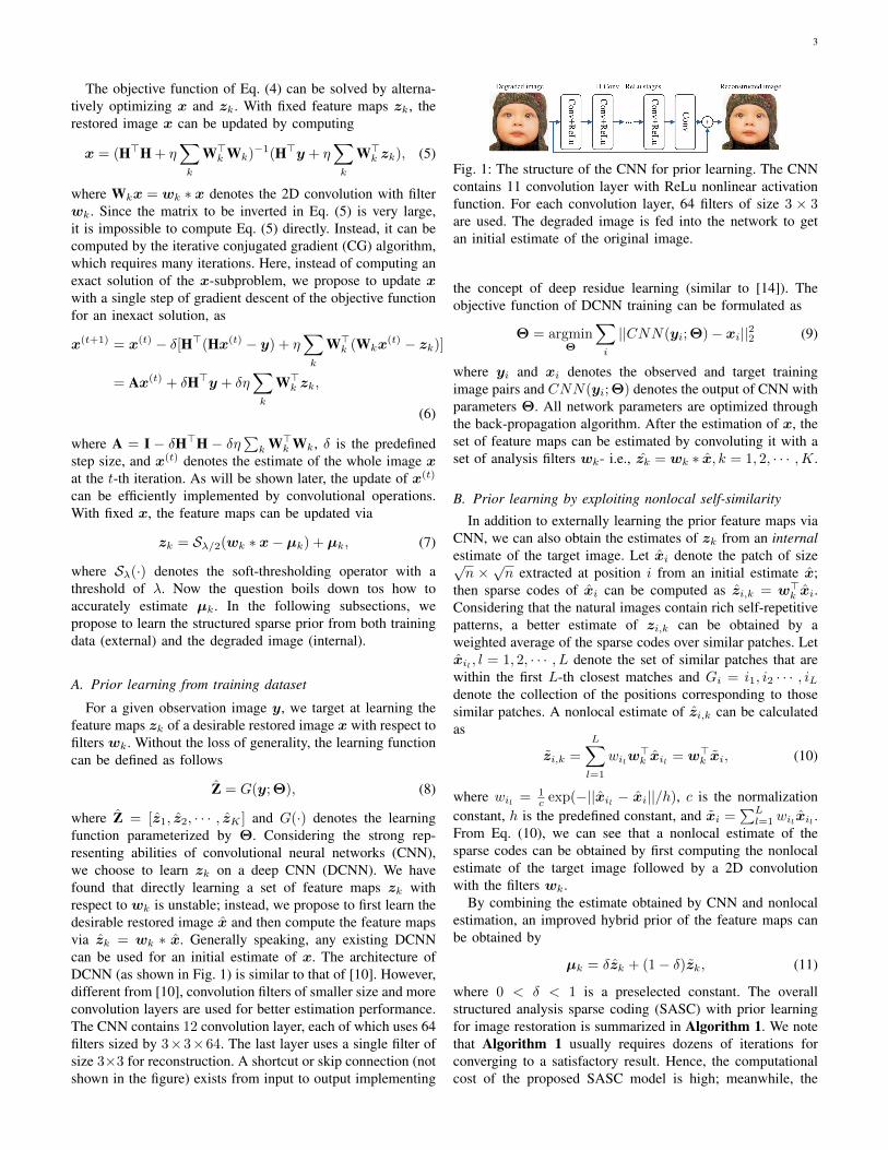
where Z = [z1, z2, · · · , zK ] and G(·) denotes the learningfunction parameterized by Θ. Considering the strong rep-resenting abilities of convolutional neural networks (CNN),we choose to learn zk on a deep CNN (DCNN). We havefound that directly learning a set of feature maps zk withrespect to wk is unstable; instead, we propose to first learn thedesirable restored image x and then compute the feature mapsvia zk = wk ∗ x. Generally speaking, any existing DCNNcan be used for an initial estimate of x. The architecture ofDCNN (as shown in Fig. 1) is similar to that of [10]. However,different from [10], convolution filters of smaller size and moreconvolution layers are used for better estimation performance.The CNN contains 12 convolution layer, each of which uses 64filters sized by 3×3×64. The last layer uses a single filter ofsize 3×3 for reconstruction. A shortcut or skip connection (notshown in the figure) exists from input to output implementing

Fig. 1: The structure of the CNN for prior learning. The CNNcontains 11 convolution layer with ReLu nonlinear activationfunction. For each convolution layer, 64 filters of size 3 × 3are used. The degraded image is fed into the network to getan initial estimate of the original image.

the concept of deep residue learning (similar to [14]). Theobjective function of DCNN training can be formulated as

Θ = argminΘ

∑i

||CNN(yi; Θ)− xi||22 (9)

where yi and xi denotes the observed and target trainingimage pairs and CNN(yi; Θ) denotes the output of CNN withparameters Θ. All network parameters are optimized throughthe back-propagation algorithm. After the estimation of x, theset of feature maps can be estimated by convoluting it with aset of analysis filters wk- i.e., zk = wk ∗ x, k = 1, 2, · · · ,K.

B. Prior learning by exploiting nonlocal self-similarity

In addition to externally learning the prior feature maps viaCNN, we can also obtain the estimates of zk from an internalestimate of the target image. Let xi denote the patch of size√n ×√n extracted at position i from an initial estimate x;

then sparse codes of xi can be computed as zi,k = w>k xi.Considering that the natural images contain rich self-repetitivepatterns, a better estimate of zi,k can be obtained by aweighted average of the sparse codes over similar patches. Letxil , l = 1, 2, · · · , L denote the set of similar patches that arewithin the first L-th closest matches and Gi = i1, i2 · · · , iLdenote the collection of the positions corresponding to thosesimilar patches. A nonlocal estimate of zi,k can be calculatedas

zi,k =

L∑l=1

wilw>k xil = w>k xi, (10)

where wil = 1c exp(−||xil − xi||/h), c is the normalization

constant, h is the predefined constant, and xi =∑Ll=1 wil xil .

From Eq. (10), we can see that a nonlocal estimate of thesparse codes can be obtained by first computing the nonlocalestimate of the target image followed by a 2D convolutionwith the filters wk.

By combining the estimate obtained by CNN and nonlocalestimation, an improved hybrid prior of the feature maps canbe obtained by

µk = δzk + (1− δ)zk, (11)

where 0 < δ < 1 is a preselected constant. The overallstructured analysis sparse coding (SASC) with prior learningfor image restoration is summarized in Algorithm 1. We notethat Algorithm 1 usually requires dozens of iterations forconverging to a satisfactory result. Hence, the computationalcost of the proposed SASC model is high; meanwhile, the

4

Algorithm 1 Image SR with structured ASCInitialization:

(a) Set parameters η and λ;(b) Compute the initial estimate x(0) by the CNN;(c) Group a set of similar patches Gi for each patch xi using

x(0);(c) Compute the prior feature maps µk using Eq. (11);

Outer loop: Iteration over t = 1, 2, · · · , T

(a) Compute the feature maps z(t)k , k = 1, · · · ,K using Eq.(7);

(b) Update the HR image x(t) via Eq. (6);(c) Update µk via Eq. (11) based on x(t);

Output: x(t).

analysis filters wk used in Algorithm 1 are kept fixed. A morecomputationally efficient implementation is to approximate theproposed SASC model by a deep neural network. Throughend-to-end training, we can jointly optimize the parameters η,λ and the analysis filters wk as will be elaborated next.

IV. NETWORK IMPLEMENTATION OF SASC FOR IMAGERESTORATION

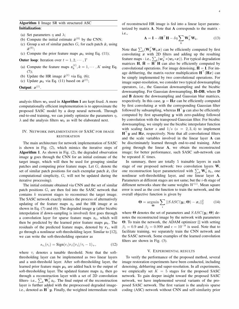
The main architecture for network implementation of SASCis shown in Fig. (2), which mimics the iterative steps ofAlgorithm 1. As shown in Fig. (2), the degraded observationimage y goes through the CNN for an initial estimate of thetarget image, which will then be used for grouping similarpatches and computing prior feature maps. Let Gi denote theset of similar patch positions for each exemplar patch xi (forcomputational simplicity, Gi will not be updated during theiterative processing).

The initial estimate obtained via CNN and the set of similarpatch positions Gi are then fed into the SASC network thatcontains k recurrent stages to reconstruct the target image.The SASC network exactly mimics the process of alternativelyupdating of the feature maps zk and the HR image x asshown in Eq. (7) and (6). The degraded image y (after bicubicinterpolation if down-sampling is involved) first goes througha convolution layer for sparse feature maps zk, which willthen be predicted by the learned prior feature maps µk. Theresiduals of the predicted feature maps, denoted by rk, willgo through a nonlinear soft-thresholding layer. Similar to [12],we can write the soft-thresholding operator as

sτi(ri) = Sign(ri)ri(|ri|/τi − 1)+, (12)

where τi denotes a tunable threshold. Note that the soft-thresholding layer can be implemented as two linear layersand a unit-threshold layer. After soft-thresholding layer, thelearned prior feature maps µk are added back to the output ofsoft-thresholding layer. The updated feature maps zk then gothrough a reconstruction layer with a set of 2D convolutionfilters- i.e.,

∑k W>k zk. The final output of the reconstruction

layer is further added with the preprocessed degraded image-i.e., denoted as H>y. Finally, the weighted intermediate result

of reconstructed HR image is fed into a linear layer parame-terized by matrix A. Note that A corresponds to the matrix -i.e.,

A = I− δH>H− δη∑k

W>k Wk. (13)

Note that∑k(W>k Wkx) can be efficiently computed by first

convoluting x with 2D filters and adding up the resultingfeature maps - i.e.,

∑k(w>k ∗(wk∗x)). For typical degradation

matrices H, H = H>H can also be efficiently computed byconvolutional operations. For image denoising, H = I. For im-age deblurring, the matrix-vector multiplication H>(Hx) canbe simply implemented by two convolutional operations. Forimage super-resolution, we consider two typical downsamplingoperators, i.e., the Gaussian downsampling and the bicubicdownsampling. For Gaussian downsampling, H=DB, where Dand B denote the downsampling and Gaussian blur matrices,respectively. In this case, y = Hx can be efficiently computedby first convoluting x with the corresponding Gaussian filterfollowed by subsampling, whereas H>y can also be efficientlycomputed by first upsampling y with zero-padding followedby convolution with the transposed Gaussian filter. For bicubicdownsampling, we simply use the bicubic interpolator functionwith scaling factor s and 1/s (s = 2, 3, 4) to implementH>y and Hx, respectively. Note that all convolutional filtersand the scale variables involved in the linear layer A canbe discriminately learned through end-to-end training. Aftergoing through the linear A, we obtain the reconstructedimage; for better performance, such SASC sub-network canbe repeated K times.

In summary, there are totally 5 trainable layers in eachstage of our proposed network: two convolution layers W,one reconstruction layer parameterized with

∑k W>k zk, one

nonlinear soft-thresholding layer, and one linear layer A.Parameters at different stages are not same; but the i-th stage ofdiffenent networks share the same weights W (i). Mean squareerror is used as the cost function to train the network, and theoverall objective function is given by

Θ = argminΘ

∑i

||SASC(yi; Θ)− xi||22 (14)

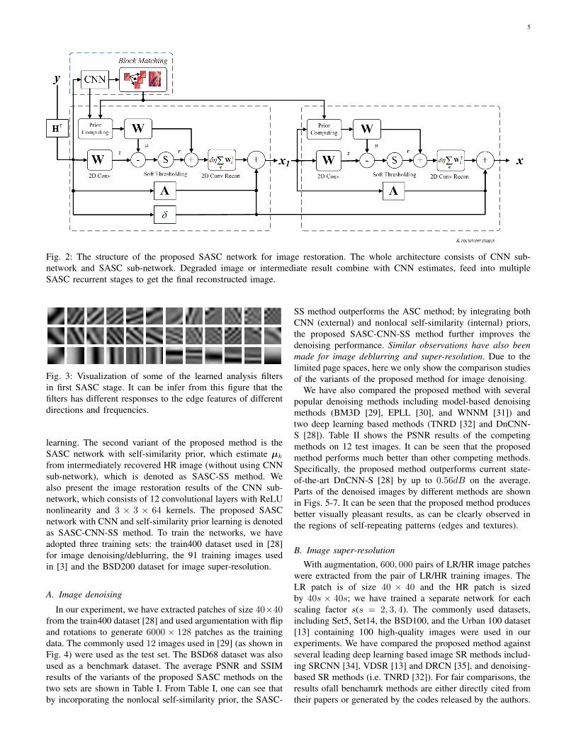
where Θ denotes the set of parameters and SASC(yi; Θ) de-notes the reconstructed image by the network with parametersΘ. To train the network, the ADAM optimizer [] with settingβ1 = 0.9 and β2 = 0.999 and ε = 10−8 is used. Note that tofacilitate training, we separately train the CNN network andthe SASC network. Some examples of the learned convolutionfilters are shown in Fig. (3).

V. EXPERIMENTAL RESULTS

To verify the performance of the proposed method, severalimage restoration experiments have been conducted, includingdenoising, deblurring and super-resolution. In all experiments,we empirically set K = 5 stages for the proposed SASCnetwork. To gain deeper insight toward the proposed SASCnetwork, we have implemented several variants of the pro-posed SASC network. The first variant is the analysis sparsecoding (ASC) network without CNN and self-similarity prior

5

Fig. 2: The structure of the proposed SASC network for image restoration. The whole architecture consists of CNN sub-network and SASC sub-network. Degraded image or intermediate result combine with CNN estimates, feed into multipleSASC recurrent stages to get the final reconstructed image.

Fig. 3: Visualization of some of the learned analysis filtersin first SASC stage. It can be infer from this figure that thefilters has different responses to the edge features of differentdirections and frequencies.

learning. The second variant of the proposed method is theSASC network with self-similarity prior, which estimate µkfrom intermediately recovered HR image (without using CNNsub-network), which is denoted as SASC-SS method. Wealso present the image restoration results of the CNN sub-network, which consists of 12 convolutional layers with ReLUnonlinearity and 3 × 3 × 64 kernels. The proposed SASCnetwork with CNN and self-similarity prior learning is denotedas SASC-CNN-SS method. To train the networks, we haveadopted three training sets: the train400 dataset used in [28]for image denoising/deblurring, the 91 training images usedin [3] and the BSD200 dataset for image super-resolution.

A. Image denoising

In our experiment, we have extracted patches of size 40×40from the train400 dataset [28] and used argumentation with flipand rotations to generate 6000 × 128 patches as the trainingdata. The commonly used 12 images used in [29] (as shown inFig. 4) were used as the test set. The BSD68 dataset was alsoused as a benchmark dataset. The average PSNR and SSIMresults of the variants of the proposed SASC methods on thetwo sets are shown in Table I. From Table I, one can see thatby incorporating the nonlocal self-similarity prior, the SASC-

SS method outperforms the ASC method; by integrating bothCNN (external) and nonlocal self-similarity (internal) priors,the proposed SASC-CNN-SS method further improves thedenoising performance. Similar observations have also beenmade for image deblurring and super-resolution. Due to thelimited page spaces, here we only show the comparison studiesof the variants of the proposed method for image denoising.

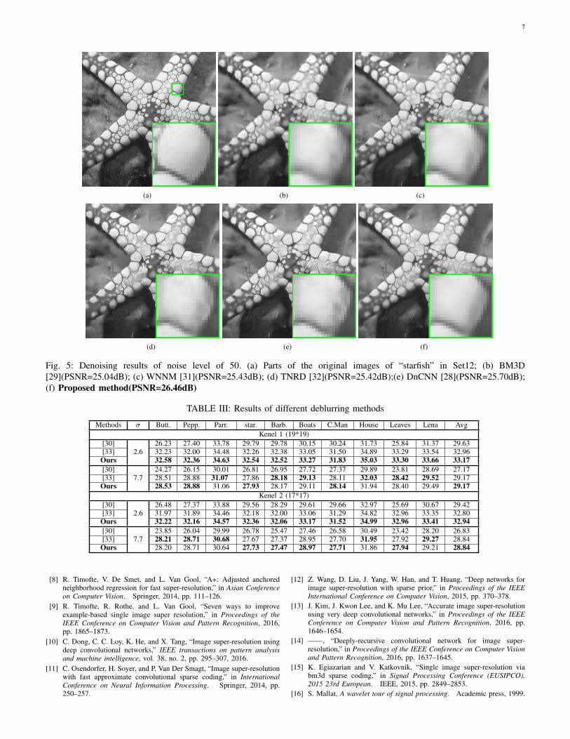
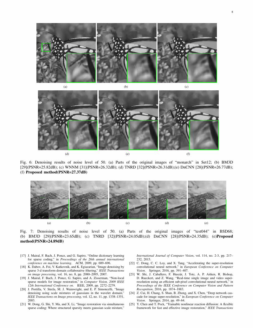
We have also compared the proposed method with severalpopular denoising methods including model-based denoisingmethods (BM3D [29], EPLL [30], and WNNM [31]) andtwo deep learning based methods (TNRD [32] and DnCNN-S [28]). Table II shows the PSNR results of the competingmethods on 12 test images. It can be seen that the proposedmethod performs much better than other competing methods.Specifically, the proposed method outperforms current state-of-the-art DnCNN-S [28] by up to 0.56dB on the average.Parts of the denoised images by different methods are shownin Figs. 5-7. It can be seen that the proposed method producesbetter visually pleasant results, as can be clearly observed inthe regions of self-repeating patterns (edges and textures).

B. Image super-resolution

With augmentation, 600, 000 pairs of LR/HR image patcheswere extracted from the pair of LR/HR training images. TheLR patch is of size 40 × 40 and the HR patch is sizedby 40s × 40s; we have trained a separate network for eachscaling factor s(s = 2, 3, 4). The commonly used datasets,including Set5, Set14, the BSD100, and the Urban 100 dataset[13] containing 100 high-quality images were used in ourexperiments. We have compared the proposed method againstseveral leading deep learning based image SR methods includ-ing SRCNN [34], VDSR [13] and DRCN [35], and denoising-based SR methods (i.e. TNRD [32]). For fair comparisons, theresults ofall benchamrk methods are either directly cited fromtheir papers or generated by the codes released by the authors.

6

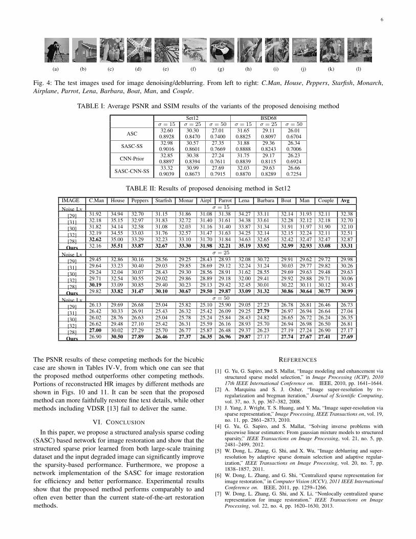
(a) (b) (c) (d) (e) (f) (g) (h) (i) (j) (k) (l)

Fig. 4: The test images used for image denoising/deblurring. From left to right: C.Man, House, Peppers, Starfish, Monarch,Airplane, Parrot, Lena, Barbara, Boat, Man, and Couple.

TABLE I: Average PSNR and SSIM results of the variants of the proposed denoising method

Set12 BSD68σ = 15 σ = 25 σ = 50 σ = 15 σ = 25 σ = 50

ASC 32.600.8928

30.300.8470

27.010.7400

31.650.8825

29.110.8097

26.010.6704

SASC-SS 32.980.9016

30.570.8601

27.350.7669

31.880.8888

29.360.8243

26.340.7006

CNN-Prior 32.850.8897

30.380.8394

27.240.7611

31.750.8839

29.170.8115

26.230.6924

SASC-CNN-SS 33.320.9039

30.990.8673

27.690.7915

32.030.8870

29.630.8289

26.660.7254

TABLE II: Results of proposed denoising method in Set12

IMAGE C.Man House Peppers Starfish Monar Airpl Parrot Lena Barbara Boat Man Couple AvgNoise Lv σ = 15

[29] 31.92 34.94 32.70 31.15 31.86 31.08 31.38 34.27 33.11 32.14 31.93 32.11 32.38

[31] 32.18 35.15 32.97 31.83 32.72 31.40 31.61 34.38 33.61 32.28 32.12 32.18 32.70

[30] 31.82 34.14 32.58 31.08 32.03 31.16 31.40 33.87 31.34 31.91 31.97 31.90 32.10

[32] 32.19 34.55 33.03 31.76 32.57 31.47 31.63 34.25 32.14 32.15 32.24 32.11 32.51

[28] 32.62 35.00 33.29 32.23 33.10 31.70 31.84 34.63 32.65 32.42 32.47 32.47 32.87

Ours 32.16 35.51 33.87 32.67 33.30 31.98 32.21 35.19 33.92 32.99 32.93 33.08 33.31Noise Lv σ = 25

[29] 29.45 32.86 30.16 28.56 29.25 28.43 28.93 32.08 30.72 29.91 29.62 29.72 29.98

[31] 29.64 33.23 30.40 29.03 29.85 28.69 29.12 32.24 31.24 30.03 29.77 29.82 30.26

[30] 29.24 32.04 30.07 28.43 29.30 28.56 28.91 31.62 28.55 29.69 29.63 29.48 29.63

[32] 29.71 32.54 30.55 29.02 29.86 28.89 29.18 32.00 29.41 29.92 29.88 29.71 30.06

[28] 30.19 33.09 30.85 29.40 30.23 29.13 29.42 32.45 30.01 30.22 30.11 30.12 30.43

Ours 29.82 33.82 31.47 30.10 30.67 29.50 29.87 33.09 31.32 30.86 30.64 30.77 30.99Noise Lv σ = 50

[29] 26.13 29.69 26.68 25.04 25.82 25.10 25.90 29.05 27.23 26.78 26.81 26.46 26.73

[31] 26.42 30.33 26.91 25.43 26.32 25.42 26.09 29.25 27.79 26.97 26.94 26.64 27.04

[30] 26.02 28.76 26.63 25.04 25.78 25.24 25.84 28.43 24.82 26.65 26.72 26.24 26.35

[32] 26.62 29.48 27.10 25.42 26.31 25.59 26.16 28.93 25.70 26.94 26.98 26.50 26.81

[28] 27.00 30.02 27.29 25.70 26.77 25.87 26.48 29.37 26.23 27.19 27.24 26.90 27.17

Ours 26.90 30.50 27.89 26.46 27.37 26.35 26.96 29.87 27.17 27.74 27.67 27.41 27.69

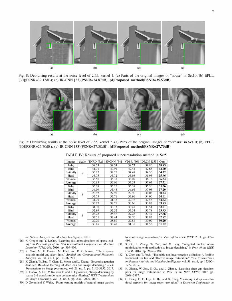
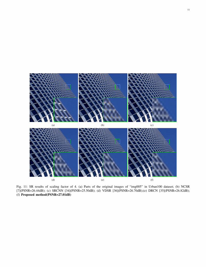
The PSNR results of these competing methods for the bicubiccase are shown in Tables IV-V, from which one can see thatthe proposed method outperforms other competing methods.Portions of reconstructed HR images by different methods areshown in Figs. 10 and 11. It can be seen that the proposedmethod can more faithfully restore fine text details, while othermethods including VDSR [13] fail to deliver the same.

VI. CONCLUSION

In this paper, we propose a structured analysis sparse coding(SASC) based network for image restoration and show that thestructured sparse prior learned from both large-scale trainingdataset and the input degraded image can significantly improvethe sparsity-based performance. Furthermore, we propose anetwork implementation of the SASC for image restorationfor efficiency and better performance. Experimental resultsshow that the proposed method performs comparably to andoften even better than the current state-of-the-art restorationmethods.

REFERENCES

[1] G. Yu, G. Sapiro, and S. Mallat, “Image modeling and enhancement viastructured sparse model selection,” in Image Processing (ICIP), 201017th IEEE International Conference on. IEEE, 2010, pp. 1641–1644.

[2] A. Marquina and S. J. Osher, “Image super-resolution by tv-regularization and bregman iteration,” Journal of Scientific Computing,vol. 37, no. 3, pp. 367–382, 2008.

[3] J. Yang, J. Wright, T. S. Huang, and Y. Ma, “Image super-resolution viasparse representation,” Image Processing, IEEE Transactions on, vol. 19,no. 11, pp. 2861–2873, 2010.

[4] G. Yu, G. Sapiro, and S. Mallat, “Solving inverse problems withpiecewise linear estimators: From gaussian mixture models to structuredsparsity,” IEEE Transactions on Image Processing, vol. 21, no. 5, pp.2481–2499, 2012.

[5] W. Dong, L. Zhang, G. Shi, and X. Wu, “Image deblurring and super-resolution by adaptive sparse domain selection and adaptive regular-ization,” IEEE Transactions on Image Processing, vol. 20, no. 7, pp.1838–1857, 2011.

[6] W. Dong, L. Zhang, and G. Shi, “Centralized sparse representation forimage restoration,” in Computer Vision (ICCV), 2011 IEEE InternationalConference on. IEEE, 2011, pp. 1259–1266.

[7] W. Dong, L. Zhang, G. Shi, and X. Li, “Nonlocally centralized sparserepresentation for image restoration.” IEEE Transactions on ImageProcessing, vol. 22, no. 4, pp. 1620–1630, 2013.

7

(a) (b) (c)

(d) (e) (f)

Fig. 5: Denoising results of noise level of 50. (a) Parts of the original images of “starfish” in Set12; (b) BM3D[29](PSNR=25.04dB); (c) WNNM [31](PSNR=25.43dB); (d) TNRD [32](PSNR=25.42dB);(e) DnCNN [28](PSNR=25.70dB);(f) Proposed method(PSNR=26.46dB)

TABLE III: Results of different deblurring methods

Methods σ Butt. Pepp. Parr. star. Barb. Boats C.Man House Leaves Lena AvgKenel 1 (19*19)

[30]2.6

26.23 27.40 33.78 29.79 29.78 30.15 30.24 31.73 25.84 31.37 29.63[33] 32.23 32.00 34.48 32.26 32.38 33.05 31.50 34.89 33.29 33.54 32.96

Ours 32.58 32.36 34.63 32.54 32.52 33.27 31.83 35.03 33.30 33.66 33.17[30]

7.724.27 26.15 30.01 26.81 26.95 27.72 27.37 29.89 23.81 28.69 27.17

[33] 28.51 28.88 31.07 27.86 28.18 29.13 28.11 32.03 28.42 29.52 29.17Ours 28.53 28.88 31.06 27.93 28.17 29.11 28.14 31.94 28.40 29.49 29.17

Kenel 2 (17*17)[30]

2.626.48 27.37 33.88 29.56 28.29 29.61 29.66 32.97 25.69 30.67 29.42

[33] 31.97 31.89 34.46 32.18 32.00 33.06 31.29 34.82 32.96 33.35 32.80Ours 32.22 32.16 34.57 32.36 32.06 33.17 31.52 34.99 32.96 33.41 32.94[30]

7.723.85 26.04 29.99 26.78 25.47 27.46 26.58 30.49 23.42 28.20 26.83

[33] 28.21 28.71 30.68 27.67 27.37 28.95 27.70 31.95 27.92 29.27 28.84Ours 28.20 28.71 30.64 27.73 27.47 28.97 27.71 31.86 27.94 29.21 28.84

[8] R. Timofte, V. De Smet, and L. Van Gool, “A+: Adjusted anchoredneighborhood regression for fast super-resolution,” in Asian Conferenceon Computer Vision. Springer, 2014, pp. 111–126.

[9] R. Timofte, R. Rothe, and L. Van Gool, “Seven ways to improveexample-based single image super resolution,” in Proceedings of theIEEE Conference on Computer Vision and Pattern Recognition, 2016,pp. 1865–1873.

[10] C. Dong, C. C. Loy, K. He, and X. Tang, “Image super-resolution usingdeep convolutional networks,” IEEE transactions on pattern analysisand machine intelligence, vol. 38, no. 2, pp. 295–307, 2016.

[11] C. Osendorfer, H. Soyer, and P. Van Der Smagt, “Image super-resolutionwith fast approximate convolutional sparse coding,” in InternationalConference on Neural Information Processing. Springer, 2014, pp.250–257.

[12] Z. Wang, D. Liu, J. Yang, W. Han, and T. Huang, “Deep networks forimage super-resolution with sparse prior,” in Proceedings of the IEEEInternational Conference on Computer Vision, 2015, pp. 370–378.

[13] J. Kim, J. Kwon Lee, and K. Mu Lee, “Accurate image super-resolutionusing very deep convolutional networks,” in Proceedings of the IEEEConference on Computer Vision and Pattern Recognition, 2016, pp.1646–1654.

[14] ——, “Deeply-recursive convolutional network for image super-resolution,” in Proceedings of the IEEE Conference on Computer Visionand Pattern Recognition, 2016, pp. 1637–1645.

[15] K. Egiazarian and V. Katkovnik, “Single image super-resolution viabm3d sparse coding,” in Signal Processing Conference (EUSIPCO),2015 23rd European. IEEE, 2015, pp. 2849–2853.

[16] S. Mallat, A wavelet tour of signal processing. Academic press, 1999.

8

(a) (b) (c)

(d) (e) (f)

Fig. 6: Denoising results of noise level of 50. (a) Parts of the original images of “monarch” in Set12; (b) BM3D[29](PSNR=25.82dB); (c) WNNM [31](PSNR=26.32dB); (d) TNRD [32](PSNR=26.31dB);(e) DnCNN [28](PSNR=26.77dB);(f) Proposed method(PSNR=27.37dB)

(a) (b) (c) (d) (e)

Fig. 7: Denoising results of noise level of 50. (a) Parts of the original images of “test044” in BSD68;(b) BM3D [29](PSNR=23.65dB); (c) TNRD [32](PSNR=24.05dB);(d) DnCNN [28](PSNR=24.35dB); (e)Proposedmethod(PSNR=24.89dB)

[17] J. Mairal, F. Bach, J. Ponce, and G. Sapiro, “Online dictionary learningfor sparse coding,” in Proceedings of the 26th annual internationalconference on machine learning. ACM, 2009, pp. 689–696.

[18] K. Dabov, A. Foi, V. Katkovnik, and K. Egiazarian, “Image denoising bysparse 3-d transform-domain collaborative filtering,” IEEE Transactionson image processing, vol. 16, no. 8, pp. 2080–2095, 2007.

[19] J. Mairal, F. Bach, J. Ponce, G. Sapiro, and A. Zisserman, “Non-localsparse models for image restoration,” in Computer Vision, 2009 IEEE12th International Conference on. IEEE, 2009, pp. 2272–2279.

[20] J. Portilla, V. Strela, M. J. Wainwright, and E. P. Simoncelli, “Imagedenoising using scale mixtures of gaussians in the wavelet domain,”IEEE Transactions on Image processing, vol. 12, no. 11, pp. 1338–1351,2003.

[21] W. Dong, G. Shi, Y. Ma, and X. Li, “Image restoration via simultaneoussparse coding: Where structured sparsity meets gaussian scale mixture,”

International Journal of Computer Vision, vol. 114, no. 2-3, pp. 217–232, 2015.

[22] C. Dong, C. C. Loy, and X. Tang, “Accelerating the super-resolutionconvolutional neural network,” in European Conference on ComputerVision. Springer, 2016, pp. 391–407.

[23] W. Shi, J. Caballero, F. Huszar, J. Totz, A. P. Aitken, R. Bishop,D. Rueckert, and Z. Wang, “Real-time single image and video super-resolution using an efficient sub-pixel convolutional neural network,” inProceedings of the IEEE Conference on Computer Vision and PatternRecognition, 2016, pp. 1874–1883.

[24] Z. Cui, H. Chang, S. Shan, B. Zhong, and X. Chen, “Deep network cas-cade for image super-resolution,” in European Conference on ComputerVision. Springer, 2014, pp. 49–64.

[25] Y. Chen and T. Pock, “Trainable nonlinear reaction diffusion: A flexibleframework for fast and effective image restoration,” IEEE Transactions

9

(a) (b) (c) (d)

Fig. 8: Deblurring results at the noise level of 2.55, kernel 1. (a) Parts of the original images of “house” in Set10; (b) EPLL[30](PSNR=32.13dB); (c) IR-CNN [33](PSNR=34.87dB); (d)Proposed method(PSNR=35.53dB)

(a) (b) (c) (d)

Fig. 9: Deblurring results at the noise level of 7.65, kernel 2. (a) Parts of the original images of “barbara” in Set10; (b) EPLL[30](PSNR=25.70dB); (c) IR-CNN [33](PSNR=27.38dB); (d)Proposed method(PSNR=27.73dB)

TABLE IV: Results of proposed super-resolution method in Set5

Images Scale TNRD [32] SRCNN [34] VDSR [36] DRCN [35] OursBaby

2

38.53 38.54 38.75 38.80 38.83Bird 41.31 40.91 42.42 42.68 42.70

Butterfly 33.17 32.75 34.49 34.56 34.72Head 35.75 35.72 35.93 35.95 35.96

Woman 35.50 35.37 36.05 36.15 36.33Average 36.85 36.66 37.53 37.63 37.71

Baby

3

35.28 35.25 35.38 35.50 35.56Bird 36.09 35.48 36.66 37.05 37.20

Butterfly 28.92 27.95 29.96 30.03 30.23Head 33.75 33.71 33.96 34.00 34.01

Woman 31.79 31.37 32.36 32.53 32.63Average 33.17 32.75 33.66 33.82 33.93

Baby

4

31.30 33.13 33.41 33.51 33.61Bird 32.99 32.52 33.54 33.78 33.93

Butterfly 26.22 25.46 27.28 27.47 27.56Head 32.51 32.44 32.70 32.82 32.82

Woman 29.20 28.89 29.81 30.09 30.20Average 30.85 30.48 31.35 31.53 31.62

on Pattern Analysis and Machine Intelligence, 2016.[26] K. Gregor and Y. LeCun, “Learning fast approximations of sparse cod-

ing,” in Proceedings of the 27th International Conference on MachineLearning (ICML-10), 2010, pp. 399–406.

[27] S. Nam, M. E. Davies, M. Elad, and R. Gribonval, “The cosparseanalysis model and algorithms,” Applied and Computational HarmonicAnalysis, vol. 34, no. 1, pp. 30–56, 2013.

[28] K. Zhang, W. Zuo, Y. Chen, D. Meng, and L. Zhang, “Beyond a gaussiandenoiser: Residual learning of deep cnn for image denoising,” IEEETransactions on image processing, vol. 26, no. 7, pp. 3142–3155, 2017.

[29] K. Dabov, A. Foi, V. Katkovnik, and K. Egiazarian, “Image denoising bysparse 3-d transform-domain collaborative filtering,” IEEE Transactionson image processing, vol. 16, no. 8, pp. 2080–2095, 2007.

[30] D. Zoran and Y. Weiss, “From learning models of natural image patches

to whole image restoration,” in Proc. of the IEEE ICCV, 2011, pp. 479–486.

[31] S. Gu, L. Zhang, W. Zuo, and X. Feng, “Weighted nuclear normminimization with application to image denoising,” in Proc. of the IEEECVPR, 2014, pp. 2862–2869.

[32] Y. Chen and T. Pock, “Trainable nonlinear reaction diffusion: A flexibleframework for fast and effective image restoration,” IEEE Transactionson Pattern Analysis and Machine Intelligence, vol. 39, no. 6, pp. 1256C–1272, 2017.

[33] K. Zhang, W. Zuo, S. Gu, and L. Zhang, “Learning deep cnn denoiserprior for image restoration,” in Proc. of the IEEE CVPR, 2017, pp.2808–2817.

[34] C. Dong, C. C. Loy, K. He, and X. Tang, “Learning a deep convolu-tional network for image super-resolution,” in European Conference on

10

TABLE V: Results of proposed super-resolution method in Set14, BSD100 and Urban100

Dataset Scale TNRD [32] SRCNN [34] VDSR [36] DRCN [35] OursPSNR SSIM PSNR SSIM PSNR SSIM PSNR SSIM PSNR SSIM

Set142 32.54 0.907 32.42 0.906 33.03 0.912 33.04 0.912 33.20 0.9143 29.46 0.823 29.28 0.821 29.77 0.831 29.76 0.831 29.96 0.8354 27.68 0.756 27.49 0.750 28.01 0.767 28.02 0.767 28.15 0.770

BSD1002 31.40 0.888 31.36 0.888 31.90 0.896 31.85 0.894 31.94 0.8963 28.50 0.788 28.41 0.786 28.80 0.796 28.80 0.795 28.88 0.7994 27.00 0.714 26.90 0.710 27.23 0.723 27.08 0.709 27.33 0.726

Urban1002 29.70 0.899 29.50 0.895 30.76 0.914 30.75 0.913 30.97 0.9153 26.44 0.807 26.24 0.799 27.15 0.828 27.08 0.824 27.33 0.8314 24.62 0.729 24.52 0.722 25.14 0.751 24.94 0.735 25.33 0.756

(a) (b) (c)

(d) (e) (f)

Fig. 10: SR results of scaling factor of 3. (a) Parts of the original images of “ppt3” in Set14; (b) NCSR[7](PSNR=25.66dB); (c) SRCNN [34](PSNR=27.04dB); (d) VDSR [36](PSNR=27.86dB);(e) DRCN [35](PSNR=27.73dB);(f) Proposed method(PSNR=28.16dB)

Computer Vision. Springer, 2014, pp. 184–199.[35] J. Kim, J. K. Lee, and K. M. Lee, “Deeply-recursive convolutional net-

work for image super-resolution,” in The IEEE Conference on ComputerVision and Pattern Recognition (CVPR Oral), June 2016.

[36] ——, “Accurate image super-resolution using very deep convolutionalnetworks,” in IEEE Conference on Computer Vision and Pattern Recog-nition, 2016, pp. 1646–1654.

11

(a) (b) (c)

(d) (e) (f)

Fig. 11: SR results of scaling factor of 4. (a) Parts of the original images of “img005” in Urban100 dataset; (b) NCSR[7](PSNR=26.44dB); (c) SRCNN [34](PSNR=25.50dB); (d) VDSR [36](PSNR=26.70dB);(e) DRCN [35](PSNR=26.82dB);(f) Proposed method(PSNR=27.01dB)