LEARNING OBJECTIVES

• Statistical tools in quality improvement• Understand how a control chart is used to detect

assignable causes• Understand how to apply pattern analysis• Construct and interpret control charts for variables• Construct and interpret control charts for attributes• Calculate and interpret process capability ratios X• Construct and interpret a cumulative sum control

chart• Use other statistical process control

Importance of Quality

• Quality of products and services has become a major decision

• Consider quality of equal importance to cost and schedule

• Quality improvement has become a major concern to many U.S. corporations

• Statistical quality control, a collection of tools that are essential in quality improvement activities

Definition of Quality• Quality means fitness for use• Expect that the products we buy will meet our

requirements• Requirements define fitness for use• Determined through the interaction of quality of

design and quality of conformance• Quality of design

– Different grades or levels of performance, reliability, serviceability

• Quality of conformance– Systematic reduction of variability and elimination of

defects

Quality Improvement

• Means the systematic elimination of waste• Waste include

– Scrap and rework in manufacturing, inspection and testing, warranty costs, and the time required to do things over again

• Can eliminate much of this waste– Lead to lower costs, higher productivity, increased

customer satisfaction, increased business reputation, higher market share, and ultimately higher profits

History of Statistical Quality Control

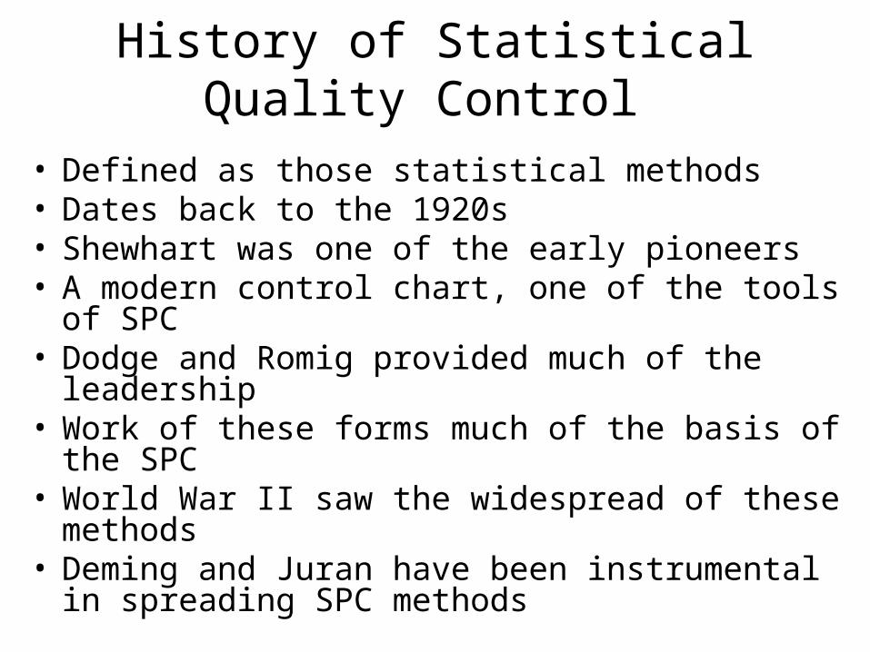
• Defined as those statistical methods• Dates back to the 1920s• Shewhart was one of the early pioneers• A modern control chart, one of the tools of SPC• Dodge and Romig provided much of the leadership • Work of these forms much of the basis of the SPC• World War II saw the widespread of these methods• Deming and Juran have been instrumental in

spreading SPC methods

Japanese and American Industry

• Japanese have been successful in deploying SPC methods

• American industry suffered extensively from Japanese competition

• Many U.S. companies have begun programs to implement these methods

Online SPC• Product must be built right the first time• Manufacturing process must be capable of

operating with little variability• Online SPC is a powerful tool• Think of statistical process control (SPC) as a

set of problem-solving tools• Major tools of SPC

– Histogram, Pareto chart, Cause-and-effect diagram, Defect-concentration diagram, Control chart, Scatter diagram, and Check sheet

• Control chart is the most powerful of the SPC tools

Natural Variability or Background Noise

• Certain amount of natural variability always exist

• Cumulative effect of many unavoidable causes

• When it is small, we consider it acceptable• Called a “stable system of chance causes.” • Operating with only chance causes of

variation present is said to be in statistical control

• Chance causes are an inherent part of the process

Assignable Causes• Other kinds of variability may be present

• Arises from three sources– Unadjusted machines, operator errors, or

defective raw materials

• Such variability is large

• Refer to these as assignable causes

• Operating in the presence of assignable causes is said to be out of control

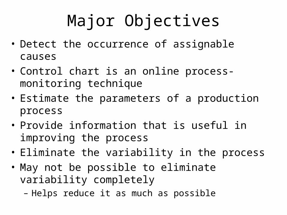
Major Objectives• Detect the occurrence of assignable causes• Control chart is an online process-monitoring

technique• Estimate the parameters of a production process• Provide information that is useful in improving the

process • Eliminate the variability in the process• May not be possible to eliminate variability

completely– Helps reduce it as much as possible

Control Chart• A typical control chart• Samples are selected

at periodic intervals• Contains a center line

(CL)• Upper control limit

(UCL) and the lower control limit (LCL)

• Point that plots outside of the control limits– Evidence that the

process is out of control

• Sample points are usually connected with straight-line segments

Nonrandom Manner of the Plots

• If they behave in a nonrandom manner– Indication that the process is out of control

• If 16 of the last 18 points plotted above the center– Very suspicious that something was wrong

• All points should have random pattern• Methods can be applied to control charts• Nonrandom pattern usually appears on a

control chart for a reason

Relationship Between Control Charts and Hypothesis testing

• Close connection between control charts and hypothesis testing

• Control chart is a test of the hypothesis

• A point within the control limits is equivalent to failing to reject the hypothesis

• A point plotting outside the control limits is equivalent to rejecting the hypothesis

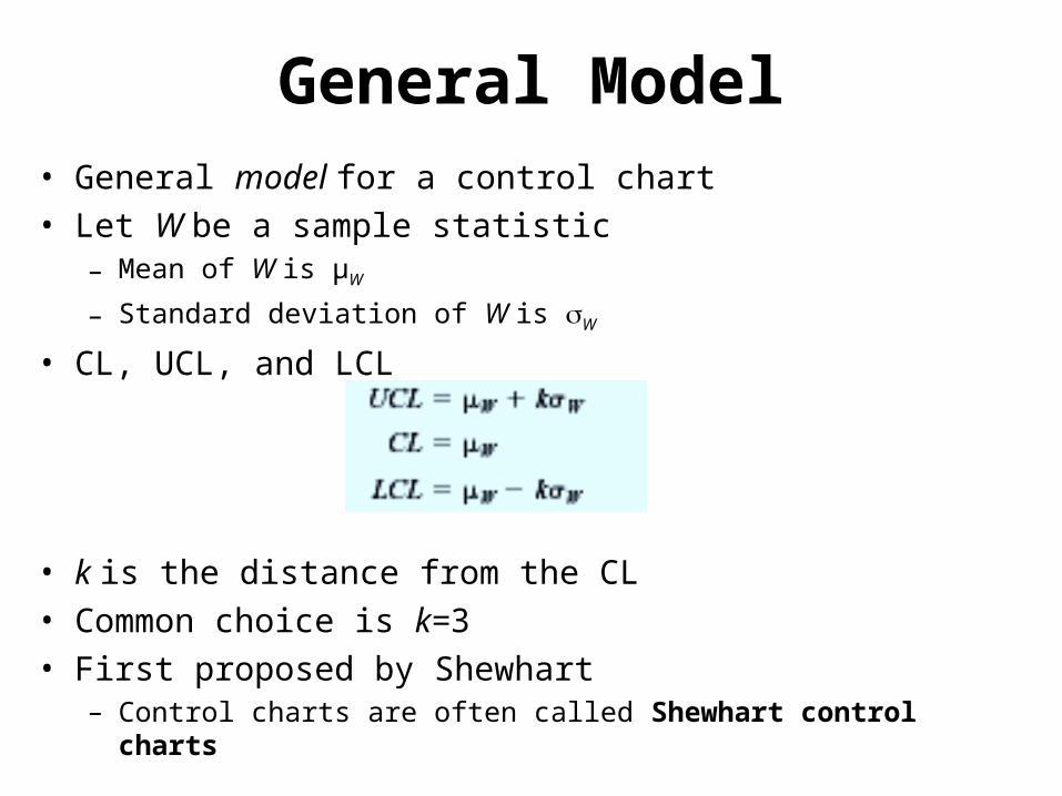
General Model• General model for a control chart• Let W be a sample statistic

– Mean of W is µW

– Standard deviation of W is W

• CL, UCL, and LCL

• k is the distance from the CL• Common choice is k=3• First proposed by Shewhart

– Control charts are often called Shewhart control charts

Use of Control Charts

• Improve the process • Identify assignable causes• If they are eliminated from the process,

variability will be reduced• May use the control chart as an estimating

device• May estimate certain process parameters• May then be used to determine the

capability of the process

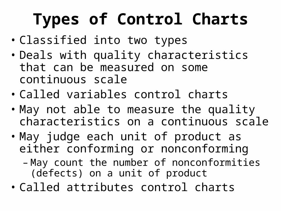
Types of Control Charts• Classified into two types• Deals with quality characteristics that can be

measured on some continuous scale• Called variables control charts• May not able to measure the quality

characteristics on a continuous scale• May judge each unit of product as either

conforming or nonconforming– May count the number of nonconformities

(defects) on a unit of product

• Called attributes control charts

Designing Control Charts• Must specify both the sample size and the

frequency of sampling• Larger samples will make it easier to detect small

shifts• Must also determine the frequency of sampling• Desirable situation would be to take large samples

very frequently• Is usually not economically feasible• Take either small samples at short intervals or

larger samples at longer intervals• Current industry practice tends to favor smaller,

more frequent samples• Increased data will increase the effectiveness of

process control

Rational Groups• Collect sample data according to the rational

subgroup

• Means that subgroups or samples – Variability of the observations includes all the

chance

• Control limits will represent bounds for all the chance variability

• Assignable causes will tend to generate points that are outside of the control limits

Two Approaches-First Approach

• Two approaches to constructing rational subgroups are used

• First approach– Consists of units that were produced at the same time

• Used when the primary purpose is to detect process shifts

• Minimizes variability within a sample• Maximizes variability between samples• Also provides better estimates of the standard

deviation of the process

Two Approaches-Second Approach

• Second approach– Consists of units of product that are

representative of all units

• Each subgroup is a random sample of all process output

• Used when the objective is to make decisions about the acceptance of all units of product

X AND R CONTROL CHARTS• X chart is the most widely used chart for monitoring

central tendency– Charts based on either the sample range or the sample

standard deviation are used to control process variability

• µ and are known – Quality characteristic has a normal distribution

• Use µ as the center line for the control chart– Place the upper and lower 3-sigma limits

• Width is inversely related to the sample size n

The 3-sigma Limits

• Utilizes the sample mean to monitor the process mean

• Choose the constant zα/2 to be 3

• Use of 3-sigma limits implies that α=0.0027

• Point plots outside the control limits when the process is in control is 0.0027

Unknown µ and

• Estimate them on the basis of preliminary samples

• CL, UCL, and LCL

• Constant A2 is tabulated for various sample sizes

R Chart• R … charts can be used to control process

variability• Can easily determine the parameters of the R …

chart• CL will obviously be the average range and the

control limits are

• r … is the sample average range, and D3 and D4

are tabulated for various sample sizes in Appendix Table X

Example

• Twenty-five samples of size 5 are drawn from a process at one-hour intervals, and the following data are obtained:

• Find trial control limits for and R chartsX

Solution

0)344.0(0

344.0

728.0)344.0(115.2

3

4

rDLCL

CL

rDUCL

rx and

344.025

60.8510.14

25

75.362 rx

312.14)344.0(577.0510.14

510.14

708.14)344.0(577.0510.14

2

2

rACLLCL

CL

rACLUCL

• Calculations for

• The trial control limits for chart are

x

• For the R chart, the trial control limits are

CONTROL CHARTS FOR INDIVIDUAL MEASUREMENTS

• Sample size used for process control is n=1• Examples

– Automated inspection and measurement technology is used– Production rate is very slow– Repeat measurements on the process differ

• In such situations, the individuals control chart is useful• Uses the moving range of two successive observations to

estimate the process variability.• Moving range is defined as• Estimate of

Control Limits

• CL, UCL, and LCL

• CL, UCL, and LCL for moving ranges

Example• Twenty successive

hardness measurements are made on a metal alloy, and the data are shown in the following table

• (a) Using all the data, compute trial control limits for individual observations and moving-range charts

• Construct the chart and plot the data

• Determine whether the process is in statistical control. If not, assume assignable causes can be found to eliminate these samples and revise the control limits.

Solution Individuals and MR(2) - Initial Study -------------------------------------------------------------------------------- • Control limits for chart I Control limits for R chart Ind.x | MR(2) ----- | ----- UCL: + 3.0 sigma = 60.8887 | UCL: + 3.0 sigma = 9.63382 Centerline = 53.05 | Centerline = 2.94737 LCL: - 3.0 sigma = 45.2113 | LCL: - 3.0 sigma = 0 | out of limits = 0 | out of limits = 0 --------------------------------------------------------------------------------• Chart: Both Normalize: No 20 subgroups, size 1 0 subgroups excluded Estimated process mean = 53.05 process sigma = 2.61292 mean MR(2) = 2.94737

X

Control Chart

0 4 8 12 16 20 45

49

53

57

61

Ind.x 53.05

60.8887

45.2113

0 4 8 12 16 20 subgroup

0

2

4

6

8

10

MR(2)

2.94737

9.63382

0

• Control chart and the moving range chart

ATTRIBUTE CONTROL CHARTS

• Classify a product as either defective or nondefective

• Achieve economy and simplicity in the inspection operation

• May judge each unit of product as either conforming or nonconforming

• Discuss the fraction-defective control chart, or P chart

P chart• D is the number of defective units• D is a binomial random variable with unknown parameter p

• Fraction defective of each sample is plotted on the chart• Variance

• CL, UCL, LCL for the P chart

• … is the observed value of the average fraction defective• Based on the normal approximation to the binomial

distribution

U Chart

• Monitor the number of defects in a unit of product• Control the number of defects• May use the control chart for defects per unit, or

the U chart• Modeled by the Poisson distribution• Sample consists of n units and there are C total

defects

Control Chart

• CL, UCL, and LCL

• is average number of defects per unit• When λ is small, the normal approximation may

not be adequate

u

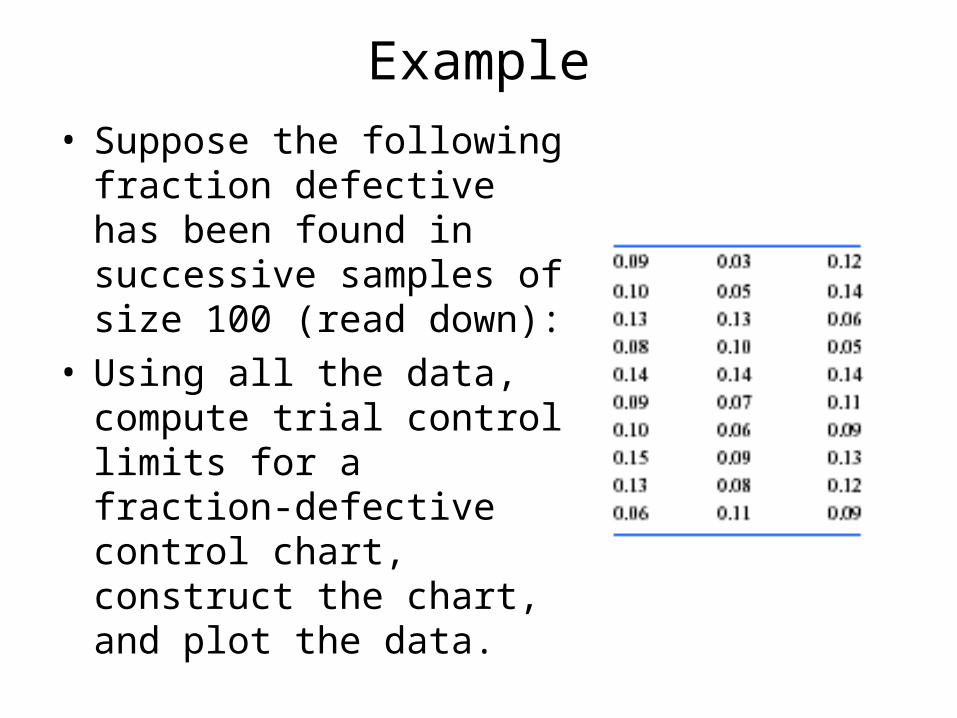
Example• Suppose the following

fraction defective has been found in successive samples of size 100 (read down):

• Using all the data, compute trial control limits for a fraction-defective control chart, construct the chart, and plot the data.

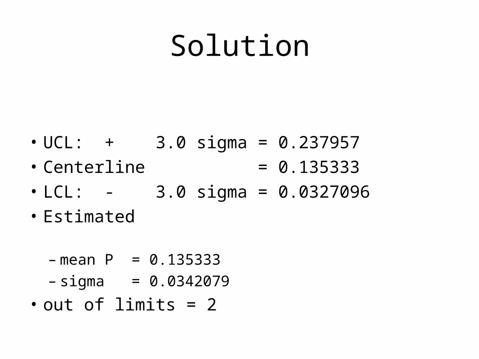
Solution

• UCL: + 3.0 sigma = 0.237957

• Centerline = 0.135333

• LCL: - 3.0 sigma = 0.0327096

• Estimated – mean P = 0.135333 – sigma = 0.0342079

• out of limits = 2

U chart

• U chart for fraction defective

0 5 10 15 20 25 30

subgroup

0

0.2

0.4

0.6

0.8

1

P

0.135333

0.237957

0.0327096