Embed Size (px)
Citation preview
Learning Optical Flow
Goren Gordon
and
Emanuel Milman
After Roth and Black:
• On the Spatial Statistics of Optical Flow, ICCV 2005.
• Fields of Experts: A Framework for Learning Image Priors, CVPR 2005.
Advanced Topics in Computer Vision
May 28, 2006
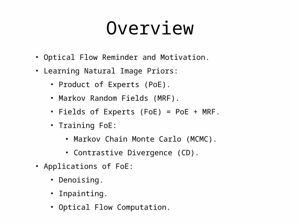
Overview• Optical Flow Reminder and Motivation.
• Learning Natural Image Priors:
• Product of Experts (PoE).
• Markov Random Fields (MRF).
• Fields of Experts (FoE) = PoE + MRF.
• Training FoE:
• Markov Chain Monte Carlo (MCMC).
• Contrastive Divergence (CD).
• Applications of FoE:
• Denoising.
• Inpainting.
• Optical Flow Computation.
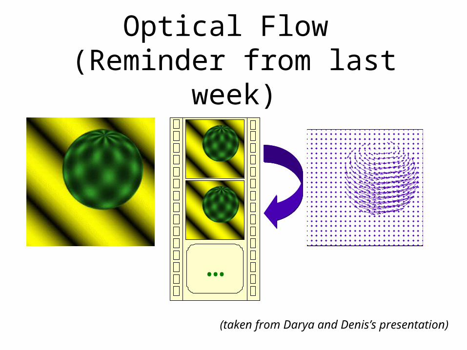
Optical Flow (Reminder from last week)
…
(taken from Darya and Denis’s presentation)
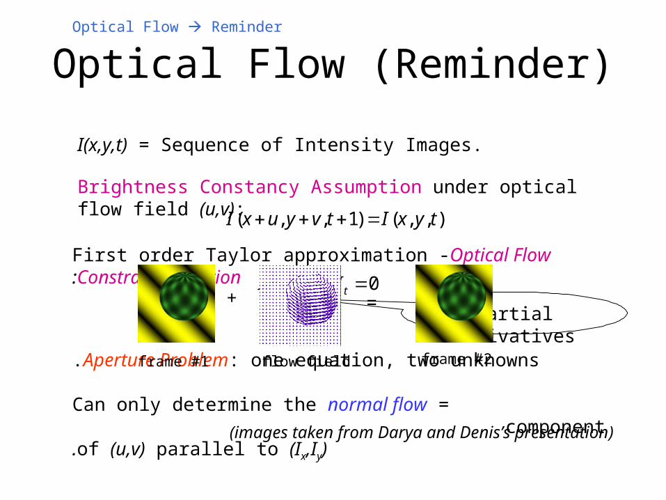
Optical Flow (Reminder)
Brightness Constancy Assumption under optical flow field )u,v(:
0 tyx IvIuI
),,()1,,( tyxItvyuxI
First order Taylor approximation -Optical Flow Constraint Equation:
Aperture Problem: one equation, two unknowns.
Can only determine the normal flow = component of )u,v( parallel to )Ix,Iy(.
I)x,y,t( = Sequence of Intensity Images.
Partial derivatives
+ =
frame #1 frame #2flow field
(images taken from Darya and Denis’s presentation)
Optical Flow Reminder
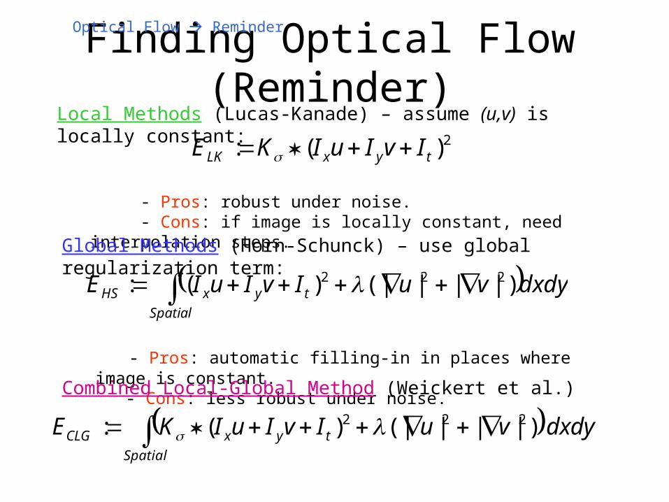
Local Methods (Lucas-Kanade) – assume )u,v( is locally constant:
- Pros: robust under noise. - Cons: if image is locally constant, need interpolation steps.
Global Methods (Horn-Schunck) – use global regularization term:
- Pros: automatic filling-in in places where image is constant. - Cons: less robust under noise.
Finding Optical Flow (Reminder)
2)(: tyxLK IvIuIKE
dxdyvuIvIuIESpatial
tyxHS )|||(|)(: 222
dxdyvuIvIuIKESpatial
tyxCLG )|||(|)(: 222
Combined Local-Global Method (Weickert et al.)
Optical Flow Reminder
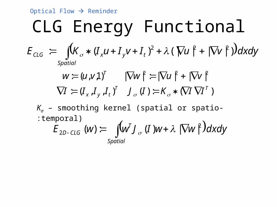
CLG Energy Functional dxdyvuIvIuIKE
Spatial
tyxCLG )|||(|)(: 222
) (:)( ),,(:
|||| : || )1,,(: 222
TTtyx
T
IIKIJIIII
vuwvuw
dxdydtwwIJwwE
dxdywwIJwwE
TemporalSpatial
TCLGD
Spatial
TCLGD
||)(:)(
||)(:)(
23
22
Kσ – smoothing kernel (spatial or spatio-temporal):
Optical Flow Reminder
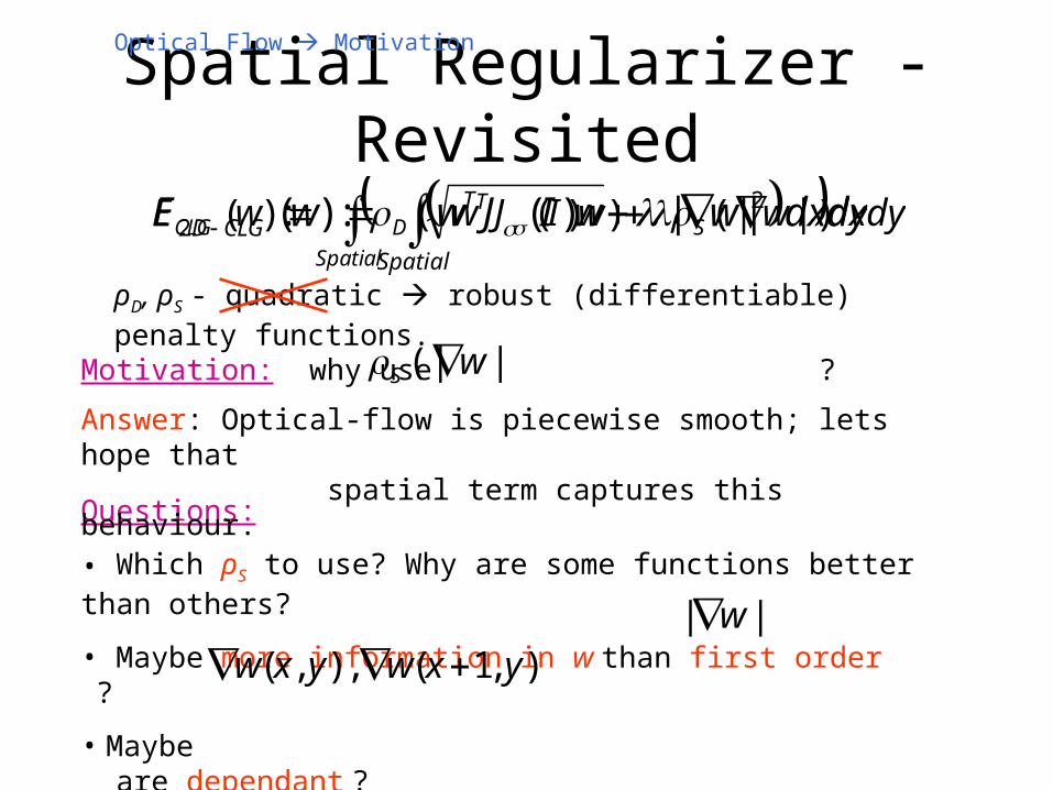
Spatial Regularizer - Revisited
dxdywwIJwwESpatial
ST
DCLG |)(|))((:)(
Questions:
• Which ρS to use? Why are some functions better than others?
• Maybe more information in w than first order ?
• Maybe are dependant ?
|| w
Motivation: why use ?|)(| wS Answer: Optical-flow is piecewise smooth; lets hope that spatial term captures this behaviour.
),1( , ),( yxwyxw
dxdywwIJwwESpatial
TCLGD ||)(:)( 2
2
ρD, ρS - quadratic robust (differentiable) penalty functions.
Optical Flow Motivation
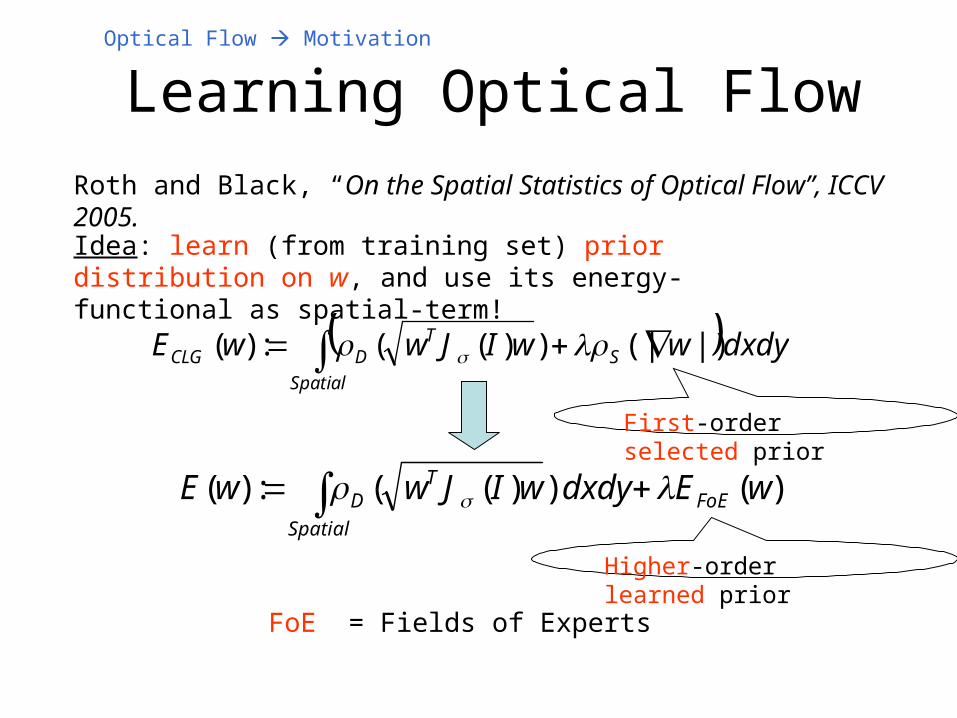
Learning Optical Flow
Roth and Black, “On the Spatial Statistics of Optical Flow”, ICCV 2005.
)( ))((:)( wEdxdywIJwwE FoE
Spatial
TD
FoE = Fields of Experts
dxdywwIJwwESpatial
ST
DCLG |)(|))((:)(
Idea: learn (from training set) prior distribution on w, and use its energy-functional as spatial-term!
First-order selected prior
Higher-order learned prior
Optical Flow Motivation
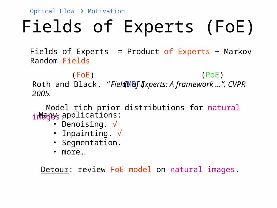
Fields of Experts (FoE)Fields of Experts = Product of Experts + Markov Random Fields
(FoE) (PoE) (MRF)
Roth and Black, “Fields of Experts: A framework …”, CVPR 2005.
Model rich prior distributions for natural images.
Detour: review FoE model on natural images.
Many applications:• Denoising. √• Inpainting. √• Segmentation.• more…
Optical Flow Motivation
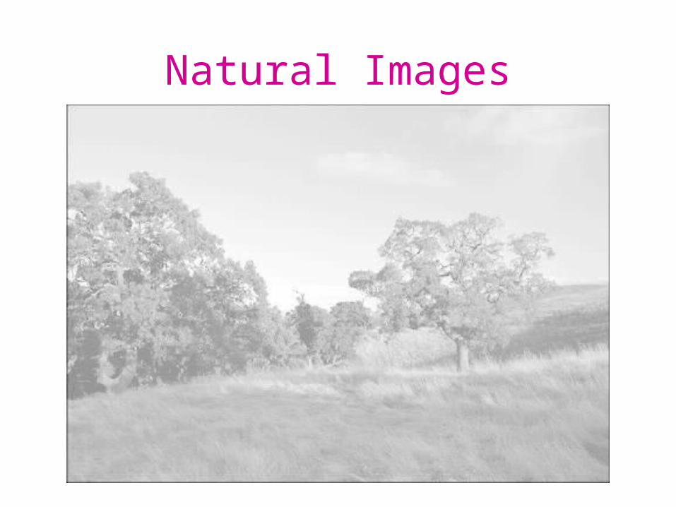
Natural Images
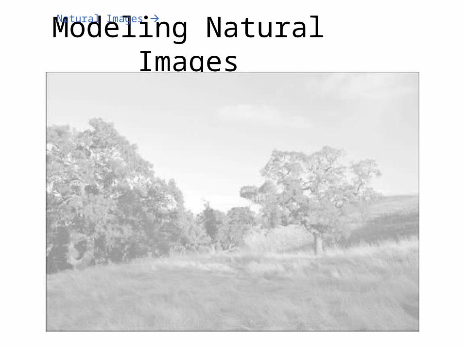
Modeling Natural Images
Challenging:
• High dimensionality ( |Ω| ≥10000 ).
• Non-Gaussian statistics (even simplest models assume MoG).
• Need to model correlations in image structure over extended neighborhoods.
Natural Images
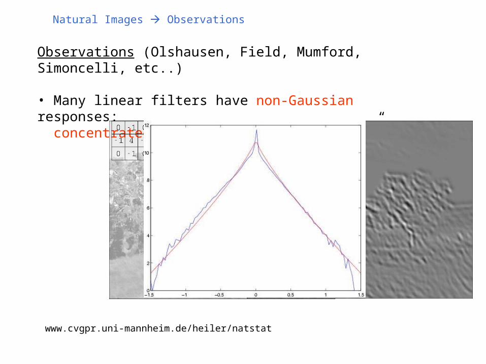
Observations (Olshausen, Field, Mumford, Simoncelli, etc..)
• Many linear filters have non-Gaussian responses: concentrated around 0 with “heavy tails”.
www.cvgpr.uni-mannheim.de/heiler/natstat
Natural Images Observations

• Statistics of image pixels are higher-order than pair-wise correlations.
• Responses of different filters are usually not independent.
Natural Images Observations
Observations (Olshausen, Field, Mumford, Simoncelli, etc..)
• Many linear filters have non-Gaussian responses: concentrated around 0 with “heavy tails”.
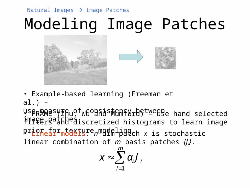
Modeling Image Patches
• Example-based learning (Freeman et al.) – use measure of consistency between image patches.
m
iiiJax
1
• FRAME (Zhu, Wu and Mumford) – use hand selected filters and discretized histograms to learn image prior for texture modeling.
• Linear models: n-dim patch x is stochastic linear combination of m basis patches {Ji}.
Natural Images Image Patches
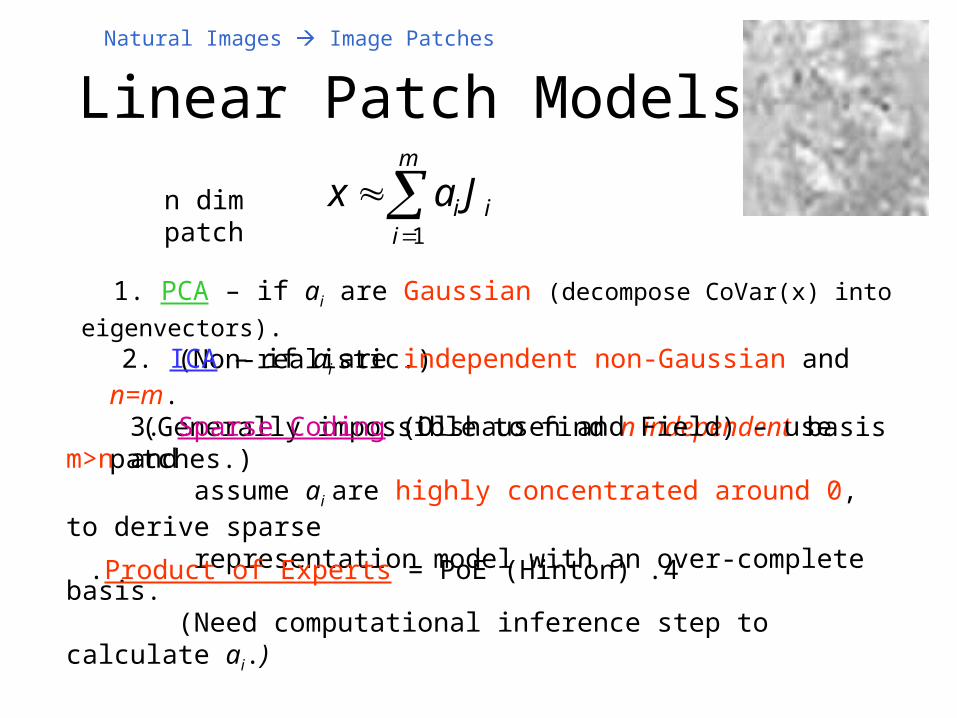
Linear Patch ModelsNatural Images Image Patches
m
iiiJax
1
1. PCA – if ai are Gaussian (decompose CoVar(x) into eigenvectors). (Non-realistic.)
2. ICA – if ai are independent non-Gaussian and n=m. (Generally impossible to find n independent basis patches.)
3. Sparse Coding (Olshausen and Field) – use m>n and assume ai are highly concentrated around 0, to derive sparse representation model with an over-complete basis. (Need computational inference step to calculate ai.(
n dim patch
4 .Product of Experts = PoE (Hinton).

Product of Experts
X X X = ?
Product of Experts (PoE)
• Model high-dim distributions as product of low-dim expert distributions.
dxxp
xpxp
i
m
ii
i
m
ii
m
) |(
) |()|(
1
11
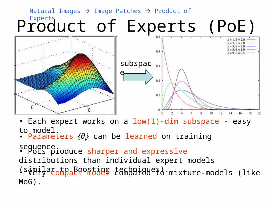
• Each expert works on a low(1)-dim subspace - easy to model.
x – data
θi – i’th expert’s parameter
• PoEs produce sharper and expressive distributions than individual expert models (similar to Boosting techniques).
• Very compact model compared to mixture-models (like MoG).
Natural Images Image Patches Product of Experts
• Parameters {θi} can be learned on training sequence.
subspace
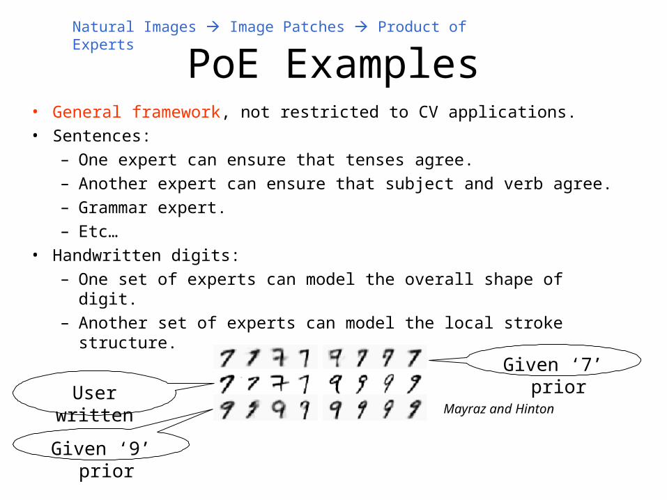
PoE Examples• General framework, not restricted to CV applications. • Sentences:
– One expert can ensure that tenses agree.– Another expert can ensure that subject and verb agree.– Grammar expert.– Etc…
• Handwritten digits:– One set of experts can model the overall shape of digit.– Another set of experts can model the local stroke structure.
Mayraz and Hinton
Natural Images Image Patches Product of Experts
User written
Given ‘9’ prior
Given ‘7’ prior

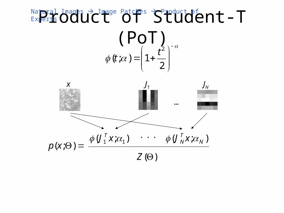
Product of Student-T (PoT)• Filter responses on images - concentrated, heavy tailed distributions.
• Welling, Hinton et al “Learning … with product of Student-t distributions”, 2003.
21);(
2tt
Natural Images Image Patches Product of Experts
Polynomial tail decay!
Model with Student-t:
Product of Student-T (PoT)
21);(
2tt
Natural Images Image Patches Product of Experts
…
);( 11 xJ T
x J1 JN
);( NTN xJ
)(Z);(xp
Product of Student-T (PoT)
21);(
2tt);(
)(
1);(
1i
Ti
N
ii xJ
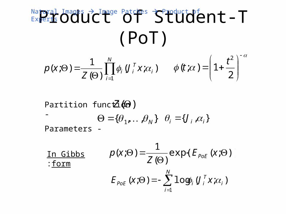
Zxp
Natural Images Image Patches Product of Experts
},,{ 1 N },{ iii J Partition function -
Parameters -
)(Z
));(exp()(
1);(
xEZ
xp PoE
);( log);(1
iTii
N
iPoE xJxE
In Gibbs form:
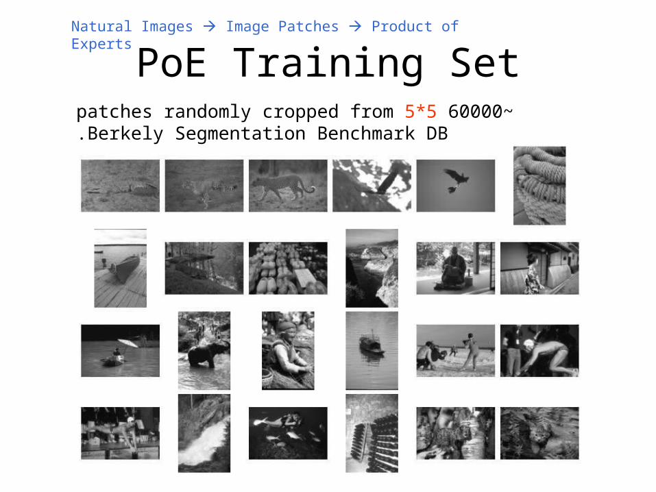
PoE Training Set~60000 5*5 patches randomly cropped from Berkely
Segmentation Benchmark DB.
Natural Images Image Patches Product of Experts

PoE Learned Filters
• Will discuss learning procedure in FoE model.
• 5*5-1=24 filters Ji were learned (no DC filter):
• Gabor-like filters accounting for local edge structures.
• Results are comparative to ICA.
• Same characteristics when training more experts.
Natural Images Image Patches Product of Experts
PoE – Final Thoughts
• Contrary to example-based approaches, the parametric representation generalizes better and beyond the training data.
• PoE permits fewer, equal or more experts than dimension.
• Over-complete case allows dependencies between different filters to be modeled, and thus more expressive than ICA.
• Product structure forces the learned filters to be “as independent as possible”, capturing different characteristics of patches.
Natural Images Image Patches Product of Experts
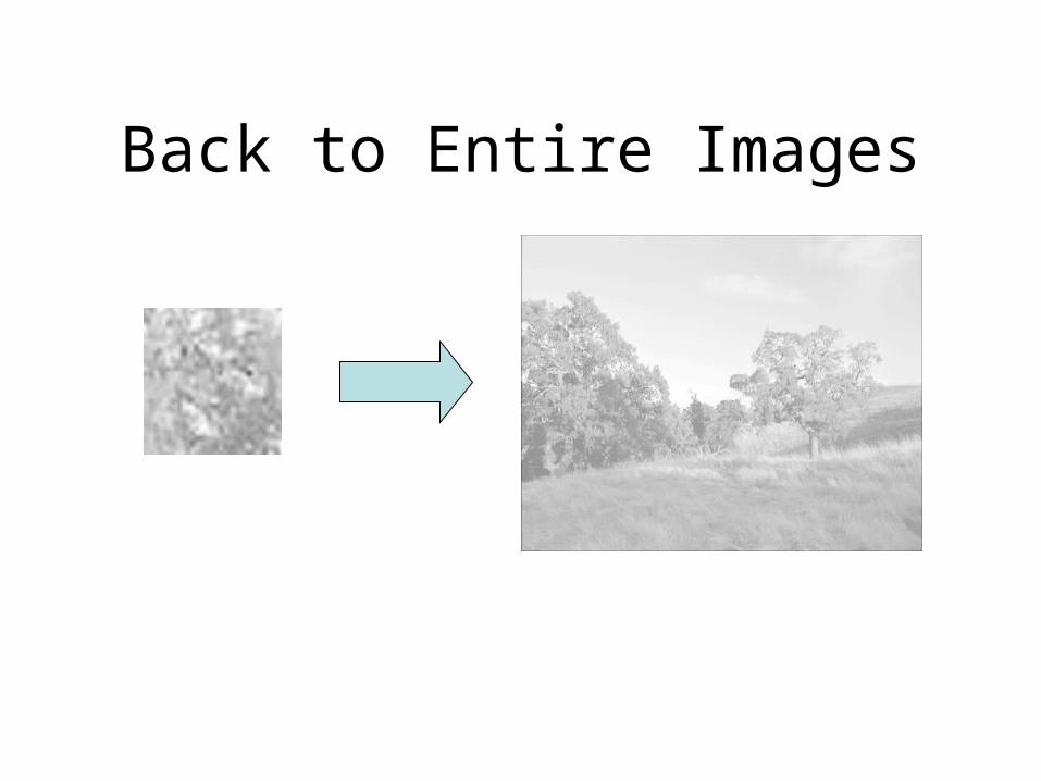
Back to Entire Images
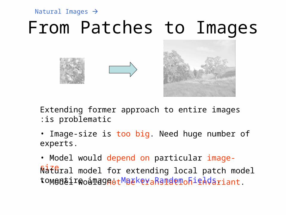
From Patches to Images
Extending former approach to entire images is problematic:
• Image-size is too big. Need huge number of experts.
• Model would depend on particular image-size.
• Model would not be translation-invariant.
Natural model for extending local patch model to entire image: Markov Random Fields.
Natural Images
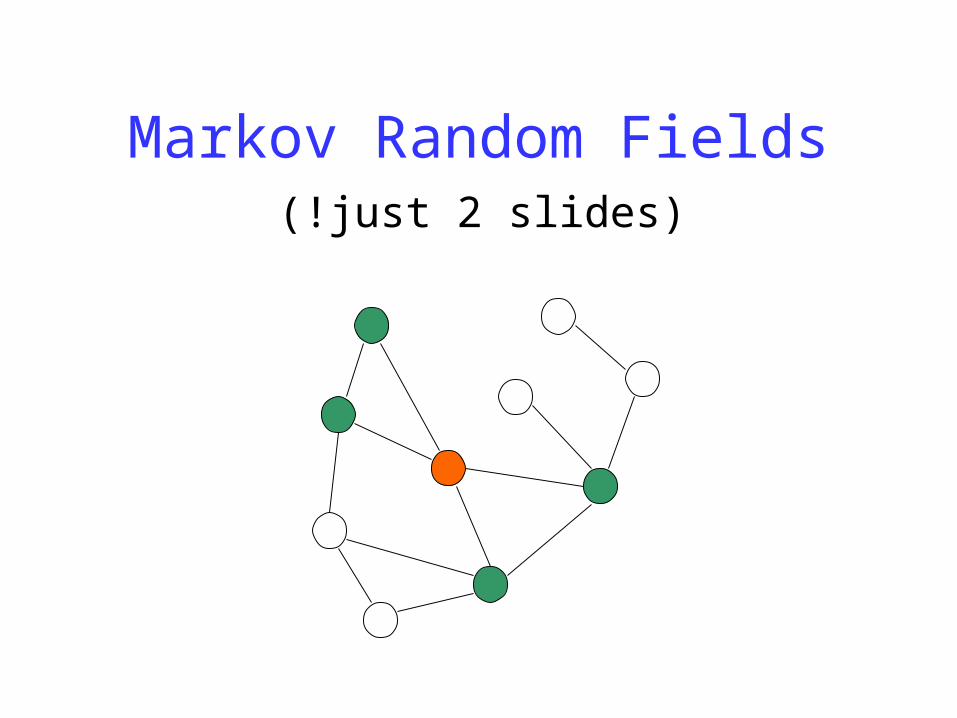
Markov Random Fields)just 2 slides(!
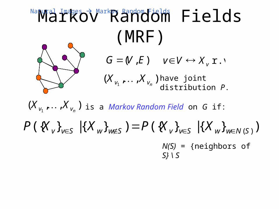
Markov Random Fields (MRF)
r.v. vXVv
),,(1 nvv XX have joint distribution P.
),( EVG
),,(1 nvv XX is a Markov Random Field on G if:
)}{|}({)}{|}({ )(SNwwSvvSwwSvv XXPXXP N)S( = {neighbors of S} \ S
Natural Images Markov Random Fields

Gibbs Distributions
P is a Gibbs distribution on X if:
)}({exp
1)( cvv
Ccc xV
ZxXP
C = set of all maximal cliques (complete sub-graphs) in G.
Vc = potential associated to clique c.
Hammersley-Clifford Theorem:
is a MRF with P>0 iff P is a Gibbs distribution. ),,(1 nvv XXX
Connects local property (MRF) with global property (Gibbs dist.)
Natural Images Markov Random Fields
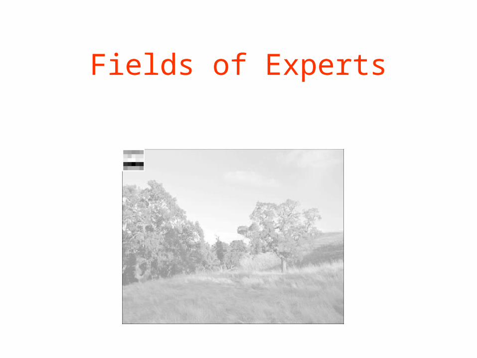
Fields of Experts
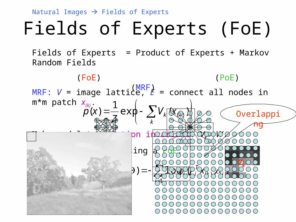
Fields of Experts (FoE)
MRF: V = image lattice, E = connect all nodes in m*m patch x)k( .
Fields of Experts = Product of Experts + Markov Random Fields
(FoE) (PoE) (MRF)
)(exp
1)( )(k
kk xV
Zxp
Make model translation invariant: Vk = W.
);( log);()( )(1
)()( ikTii
N
ikPoEk xJxExW
Model potential W using a PoE:
Natural Images Fields of Experts
Vk
Overlapping
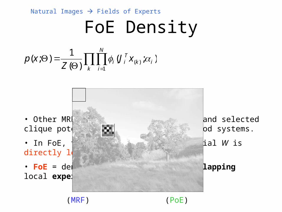
FoE Density
k
ikTii
N
iFoE xJxE );( log);( )(
1
));(exp()(
1);(
)(
1);( )(
1
xEZ
xJZ
xp FoEk
ikTi
N
ii
• Other MRF approaches typically use hand selected clique potentials and small neighborhood systems.
• In FoE, translation invariant potential W is directly learned from training images.
• FoE = density is combination of overlapping local experts.
(MRF) (PoE)
Natural Images Fields of Experts
FoE Model Pros
• Overcomes previously mentioned problems:
- Parameters Θ depend only on patch’s dimensions.
- Applies to images of arbitrary size.
- Translation invariant by definition.
• Explicitly models overlap of patches, by learning from training images.
• Overlapping patches are highly correlated; learned filters Ji and αi must account for this
Natural Images Fields of Experts
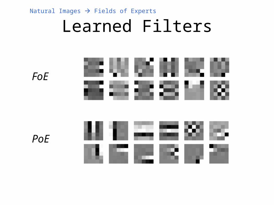
Learned Filters
FoE
PoE
Natural Images Fields of Experts
Training FoE
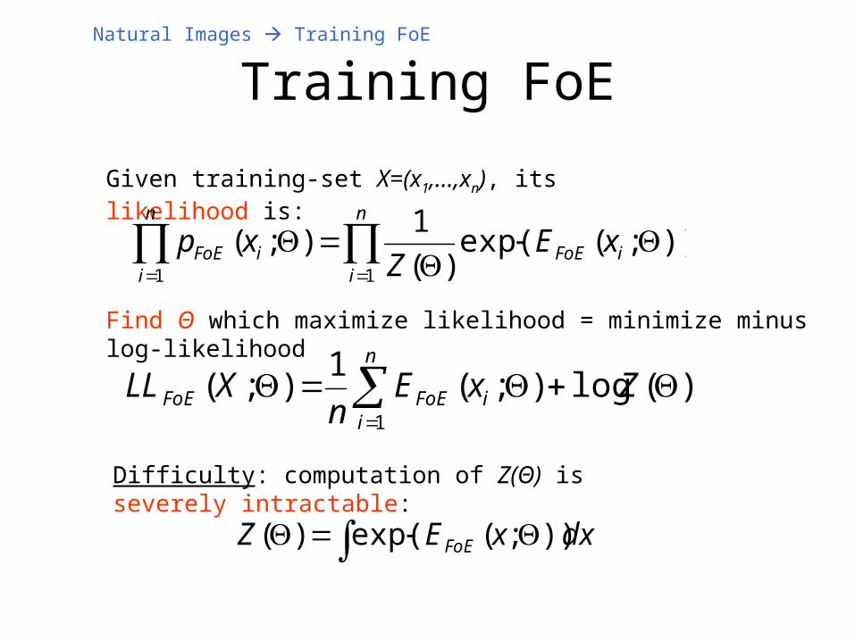
Training FoE
Given training-set X=)x1,…,xn(, its likelihood is:
));(exp()(
1);(
11
iFoE
n
i
n
iiFoE xE
Zxp
Find Θ which maximize likelihood = minimize minus log-likelihood
)(log);(1
);(1
ZxEn
XLL i
n
iFoEFoE
dxxEZ FoE ));(exp()(
Difficulty: computation of Z)Θ( is severely intractable:
Natural Images Training FoE
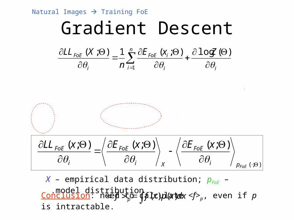
Gradient Descent
i
n
i i
iFoE
i
FoE ZxE
n
XLL
)(log);(1);(
1
dxxpxE
dxxExE
Z
dxxEZ
Z
Z
Z
FoEi
FoEFoE
i
FoE
FoEiii
);();(
));(exp();(
)(
1
));(exp()(
1)(
)(
1)(log
);(
);();();(
FoEpi
FoE
Xi
FoE
i
FoE xExExLL
X – empirical data distribution; pFoE – model distribution .
Conclusion: need to calculate <f>p, even if p is intractable.
Natural Images Training FoE
dxxpxff p )()(
Markov Chain Monte Carlo(3 Slide Detour)
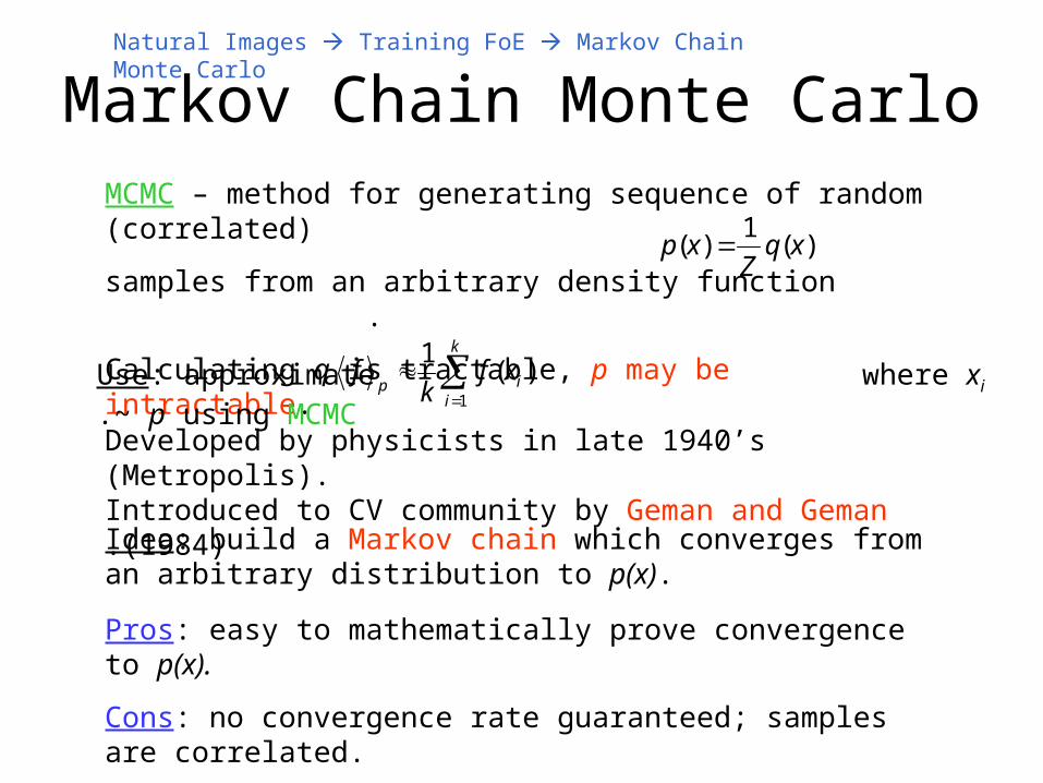
Markov Chain Monte CarloMCMC – method for generating sequence of random (correlated)
samples from an arbitrary density function .
Calculating q is tractable, p may be intractable.
)(1
)( xqZ
xp
Developed by physicists in late 1940’s (Metropolis).Introduced to CV community by Geman and Geman (1984).
Idea: build a Markov chain which converges from an arbitrary distribution to p)x(.
Pros: easy to mathematically prove convergence to p)x(.
Cons: no convergence rate guaranteed; samples are correlated.
k
iipxf
kf
1
)(1
Natural Images Training FoE Markov Chain Monte Carlo
Use: approximate where xi ~ p using MCMC.
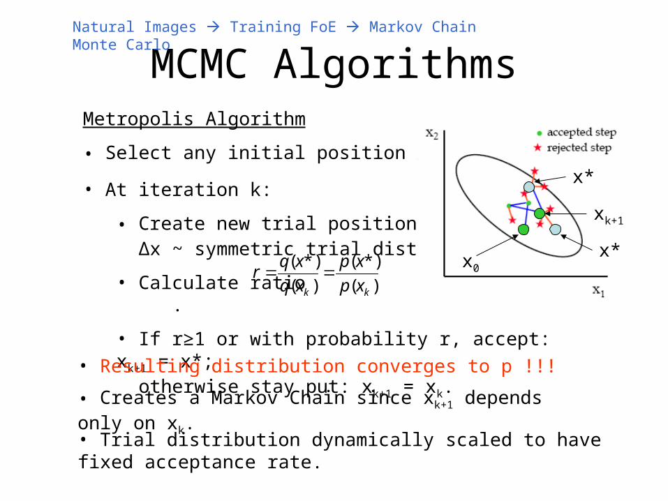
MCMC AlgorithmsMetropolis Algorithm
• Select any initial position x0.
• At iteration k:
• Create new trial position x* = xk+∆x, ∆x ~ symmetric trial distribution.
• Calculate ratio .
• If r≥1 or with probability r, accept: xk+1 = x*; otherwise stay put: xk+1 = xk.
• Trial distribution dynamically scaled to have fixed acceptance rate.
• Creates a Markov Chain since xk+1 depends only on xk.
Natural Images Training FoE Markov Chain Monte Carlo
)(
*)(
)(
*)(
kk xp
xp
xq
xqr
xk
x*
x0
x*
xk+1
• Resulting distribution converges to p !!!

Gibbs Sampler (Geman and Geman):
• Vary only one coordinate of x at a time.
• Draw new value of xj from conditional p)xj | x1,..,xj-1,xj+1,..,xn( - usually tractable when p is a MRF.
Natural Images Training FoE Markov Chain Monte Carlo
MCMC Algorithms
Hamiltonian Hybrid Monte Carlo (HMC):
• State of the art; very efficient.
• Details omitted.
Other algorithms to build sampling Markov chain:
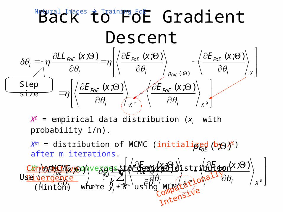
Back to FoE Gradient Descent
Xi
FoE
pi
FoE
i
FoEi
xExExLL
FoE
);();();(
);(
X0 = empirical data distribution (xi with probability 1/n).
Xm = distribution of MCMC (initialized by X0) after m iterations.
X∞ = MCMC converges to desired distribution . ); ( FoEp
0
);();(
Xi
FoE
Xi
FoE xExE
0
);();(
Xi
FoE
Xi
FoEi
xExE
m Contrastive Divergence
(Hinton)
Step size
Natural Images Training FoE
k
j i
jFoE
Xi
FoEyE
k
xE
1
);(1);(
Use where yj ~ X∞ using MCMC.
Computationally Intensive
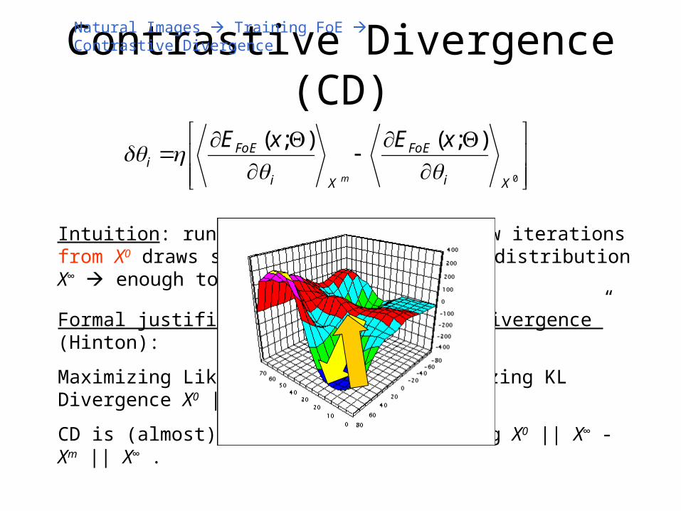
Contrastive Divergence (CD)
Intuition: running MCMC sampler for few iterations from X0 draws samples closer to target distribution X∞ enough to “feel” gradient.
Formal justification of “Contrastive Divergence” (Hinton):
Maximizing Likelihood p(X0|X∞) = Minimizing KL Divergence X0 || X∞
CD is (almost) equivalent to minimizing X0 || X∞ - Xm || X∞ .
0
);();(
Xi
FoE
Xi
FoEi
xExE
m
Natural Images Training FoE Contrastive Divergence
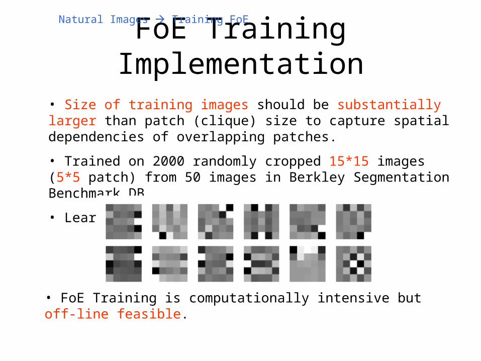
FoE Training Implementation
• Size of training images should be substantially larger than patch (clique) size to capture spatial dependencies of overlapping patches.
• Trained on 2000 randomly cropped 15*15 images (5*5 patch) from 50 images in Berkley Segmentation Benchmark DB.
• Learned 24 expert filters.
Natural Images Training FoE
• FoE Training is computationally intensive but off-line feasible.
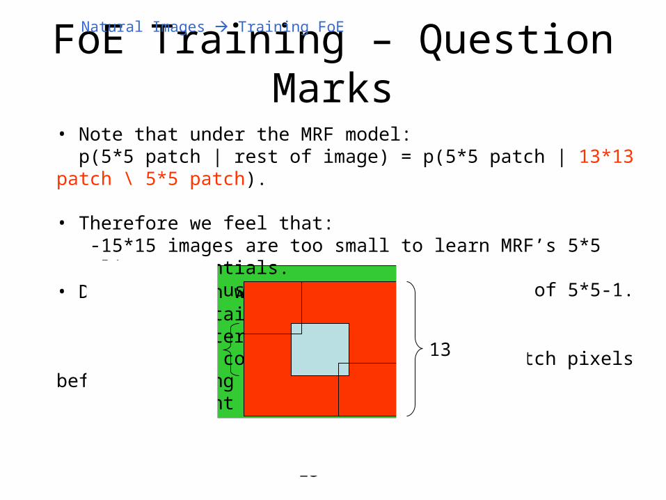
FoE Training – Question Marks
• Note that under the MRF model: p(5*5 patch | rest of image) = p(5*5 patch | 13*13 patch \ 5*5 patch). • Therefore we feel that:
-15*15 images are too small to learn MRF’s 5*5 clique potentials.- Better to use 13*13-1 filters instead of 5*5-1.
• Details which were omitted: - HMC details. - Parameter values. - Faster convergence by whitening patch pixels before computing gradient updates.
Natural Images Training FoE
5
15
13

Applications!
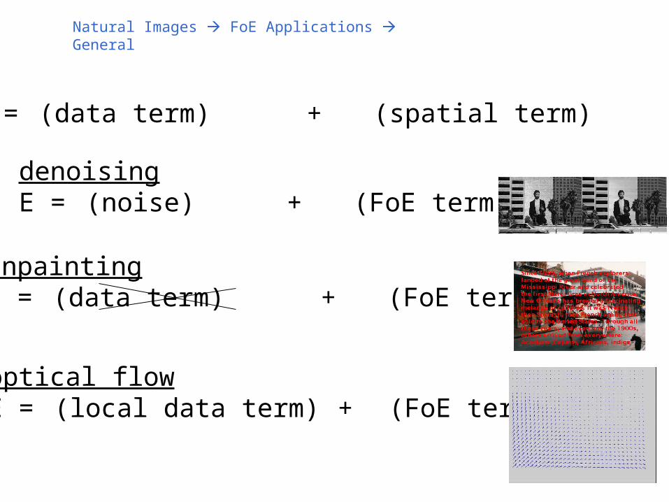
Natural Images FoE Applications General
E = (data term) + (spatial term)
denoisingE = (noise) + (FoE term)
inpaintingE = (data term) + (FoE term)
optical flowE = (local data term) + (FoE term)
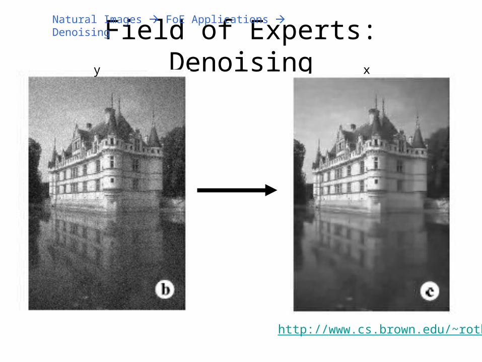
Field of Experts: Denoising
http://www.cs.brown.edu/~roth/
y x
Natural Images FoE Applications Denoising
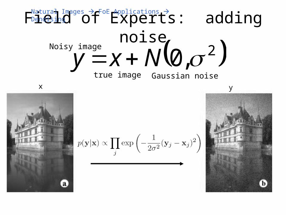
Field of Experts: adding noise
yx
Natural Images FoE Applications Denoising
2,0 Nxy true image Gaussian noise
Noisy image
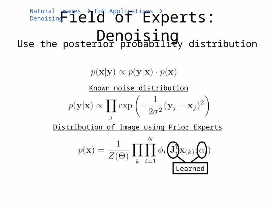
Field of Experts: DenoisingUse the posterior probability distribution
Known noise distribution
Distribution of Image using Prior Experts
Learned
Natural Images FoE Applications Denoising

Field of Experts: Denoising
Use gradient ascent
xpxypyxLL log|log)|(
Natural Images FoE Applications Denoising
Find x which maximize probability = minimize minus log-likelihood
xpxyyxLL xxx log1
| 2
2
Gradient descent of minus log-likelihood
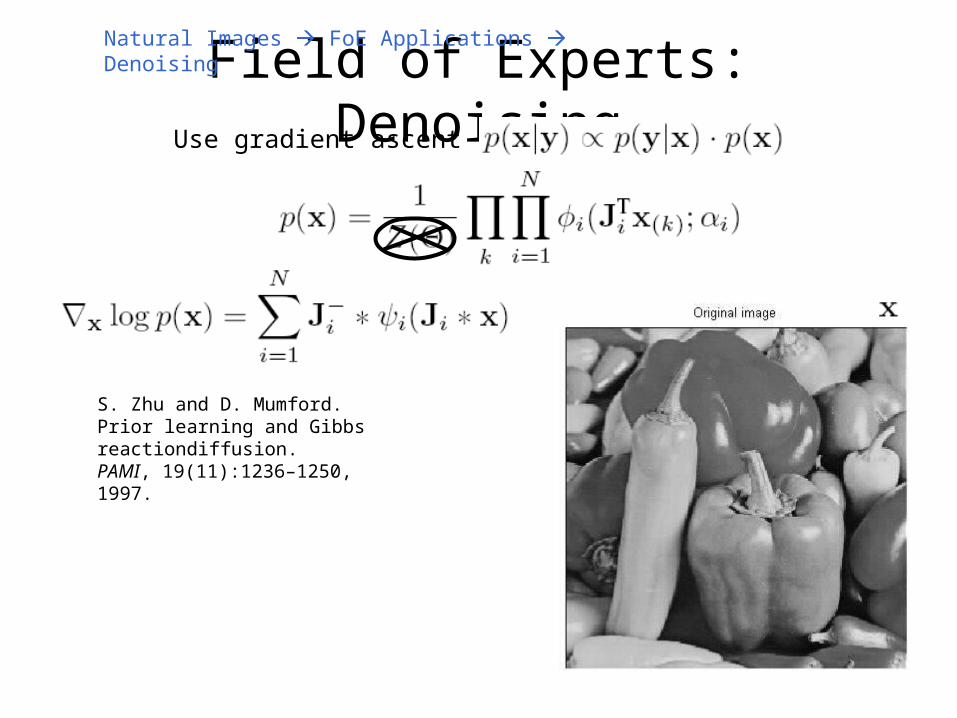
Field of Experts: DenoisingUse gradient ascent
S. Zhu and D. Mumford. Prior learning and Gibbs reactiondiffusion.PAMI, 19(11):1236–1250, 1997.
Natural Images FoE Applications Denoising
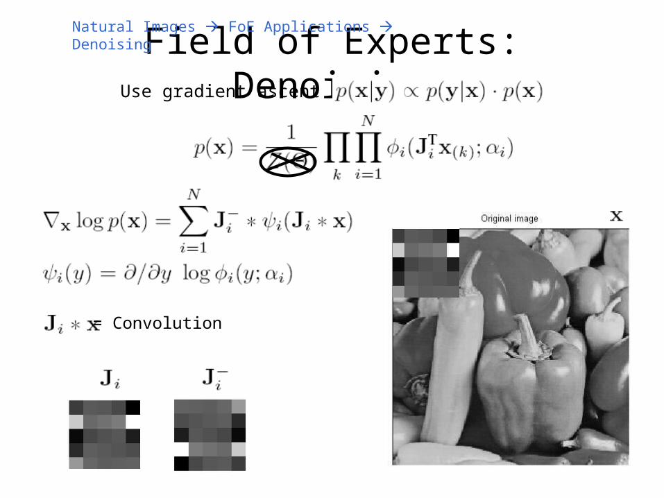
Field of Experts: DenoisingUse gradient ascent
= Convolution
Natural Images FoE Applications Denoising

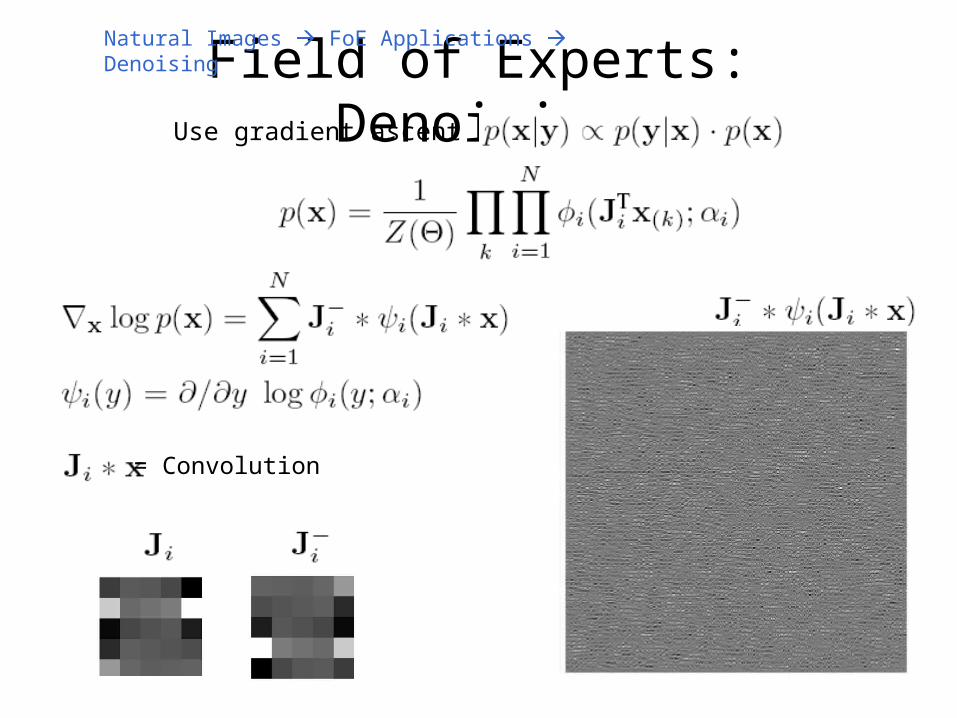
Field of Experts: DenoisingUse gradient ascent
= Convolution
Natural Images FoE Applications Denoising

Field of Experts: DenoisingUse gradient ascent
= Convolution
Natural Images FoE Applications Denoising
Field of Experts: DenoisingUse gradient ascent
= Convolution
Natural Images FoE Applications Denoising
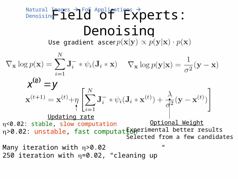
Field of Experts: DenoisingUse gradient ascent
Updating rate<0.02: stable, slow computation>0.02: unstable, fast computation
Many iteration with >0.02250 iteration with =0.02, “cleaning up”
Optional WeightExperimental better resultsSelected from a few candidates
Natural Images FoE Applications Denoising
yx 0

Field of Experts: DenoisingNatural Images FoE Applications Denoising
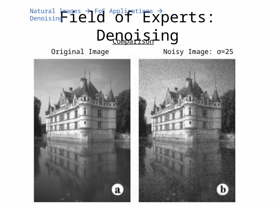
Field of Experts: Denoising
Original Image Noisy Image: σ=25
Comparison
Natural Images FoE Applications Denoising

Field of Experts: Denoising
Field of ExpertsPSNR=28.72dB
J. Portilla, V. Strela, M. Wainwright, and E. Simoncelli.IEEE Trans. Image Proc., 12(11):1338–1351, 2003
Non-linear diffusionPSNR=27.18dB
Comparison
Wavelet approachPSNR=28.90dB
J.Weickert. Scale-Space Theory in Computer Vision, pp. 3–28, 1997.
Natural Images FoE Applications Denoising
Advantages of FoE
• Compared to non-Linear Diffusion:– Uses many more filters– Obtained filters in a principled way
• Compared to wavelets:– Some results are even better – Prior trained on different data– Increased database can improve results
Natural Images FoE Applications Denoising
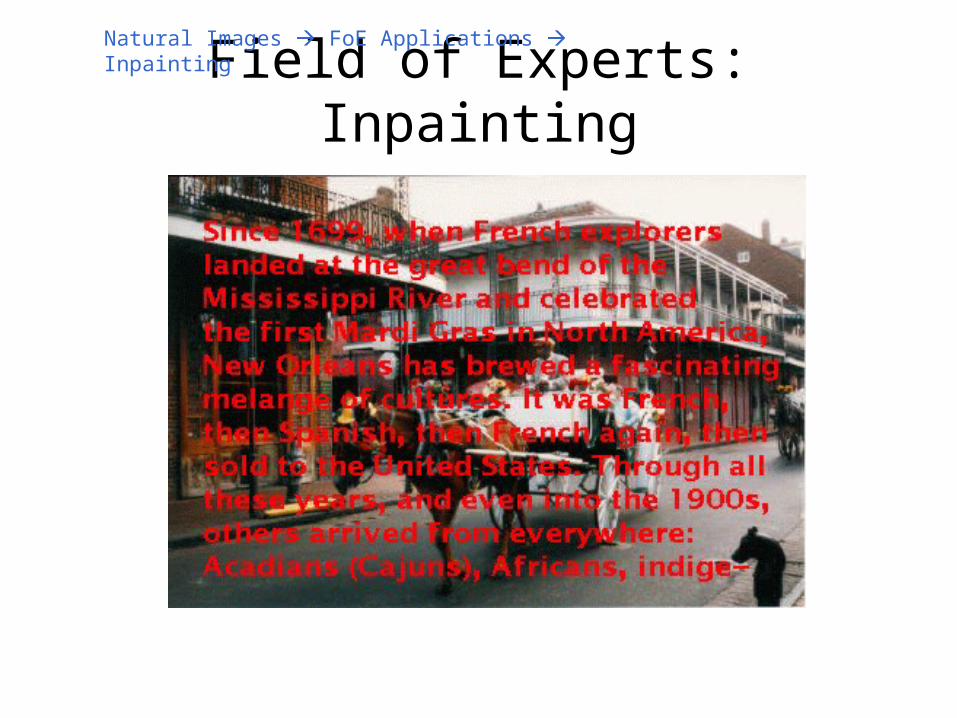
Field of Experts: InpaintingNatural Images FoE Applications Inpainting
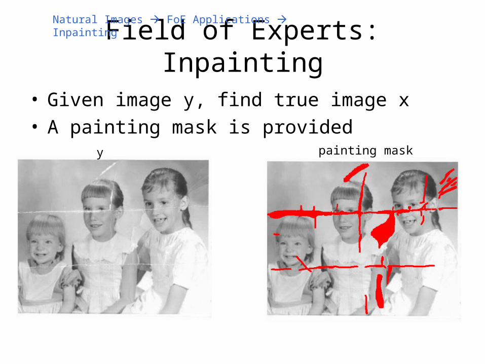
Field of Experts: Inpainting
• Given image y, find true image x• A painting mask is provided
y painting mask
Natural Images FoE Applications Inpainting

InpaintingNatural Images FoE Applications Inpainting
Diffusion Techniques
M. Bertalmıo et al. Image inpainting. ACM SIGGRAPH, pp. 417–424, 2000

Field of Experts: Inpaintingp(y) p(x)
mask inside 1
mask outsided 0M
Natural Images FoE Applications Inpainting
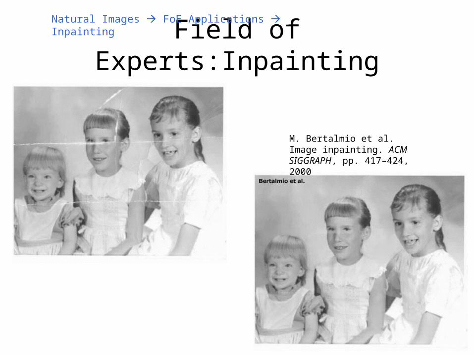
Field of Experts:Inpainting
M. Bertalmio et al. Image inpainting. ACM SIGGRAPH, pp. 417–424, 2000
Natural Images FoE Applications Inpainting
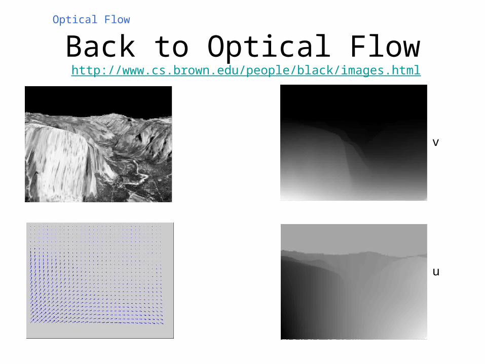
Back to Optical Flow
u
v
Optical Flow
http://www.cs.brown.edu/people/black/images.html
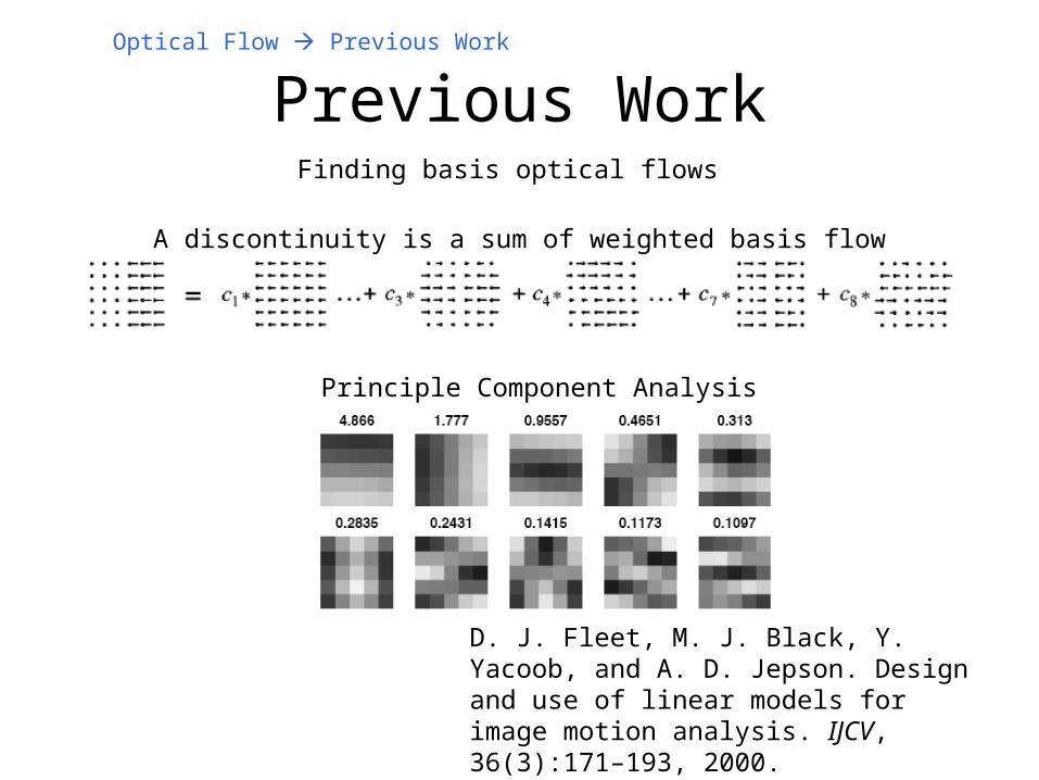
Previous Work
D. J. Fleet, M. J. Black, Y. Yacoob, and A. D. Jepson. Design and use of linear models for image motion analysis. IJCV,36(3):171–193, 2000.
Finding basis optical flows
A discontinuity is a sum of weighted basis flow
Principle Component Analysis
Optical Flow Previous Work
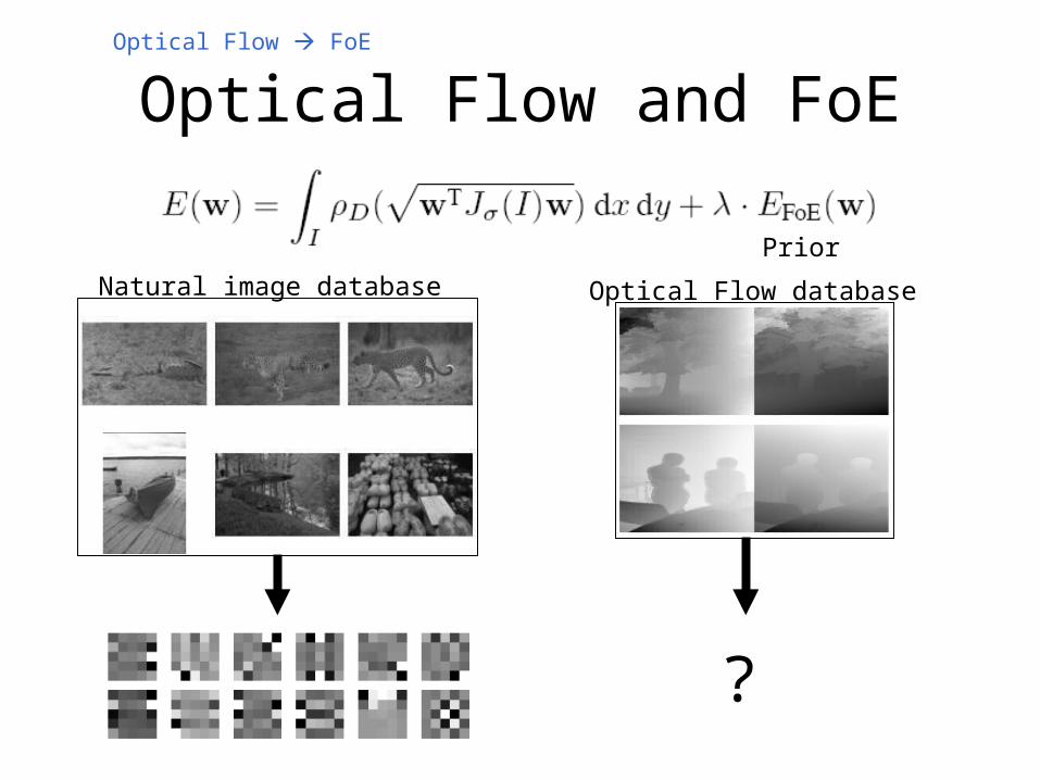
Optical Flow and FoE
Prior
Natural image database Optical Flow database
?
Optical Flow FoE

Optical Flow and Field of Experts
• Required statistics: for good experts
• Required database: for training
Database
Optical Flow FoE Database
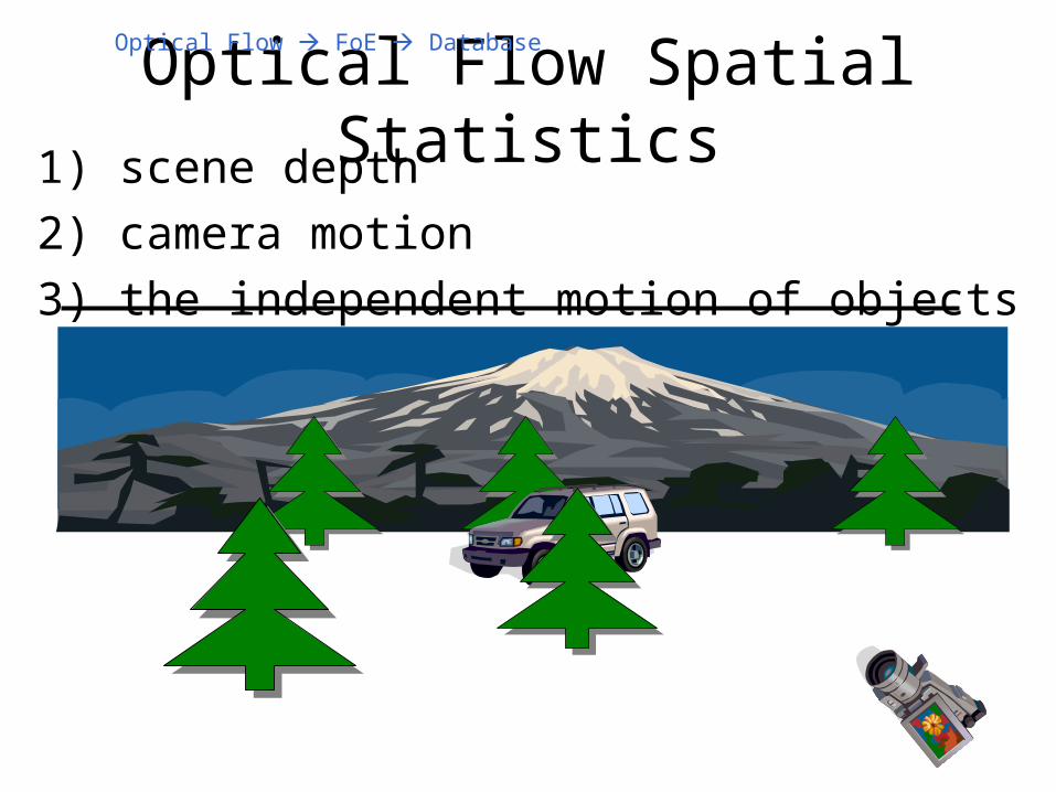
Optical Flow Spatial Statistics1) scene depth
2) camera motion
3) the independent motion of objects
Optical Flow FoE Database
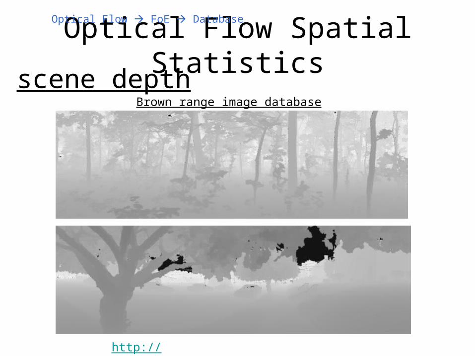
Optical Flow Spatial Statistics
http://www.dam.brown.edu/ptg/brid/index.html
Brown range image database
scene depth
Optical Flow FoE Database

Optical Flow Spatial Statistics
http://www.dam.brown.edu/ptg/brid/index.html
Brown range image database
scene depth
Optical Flow FoE Database
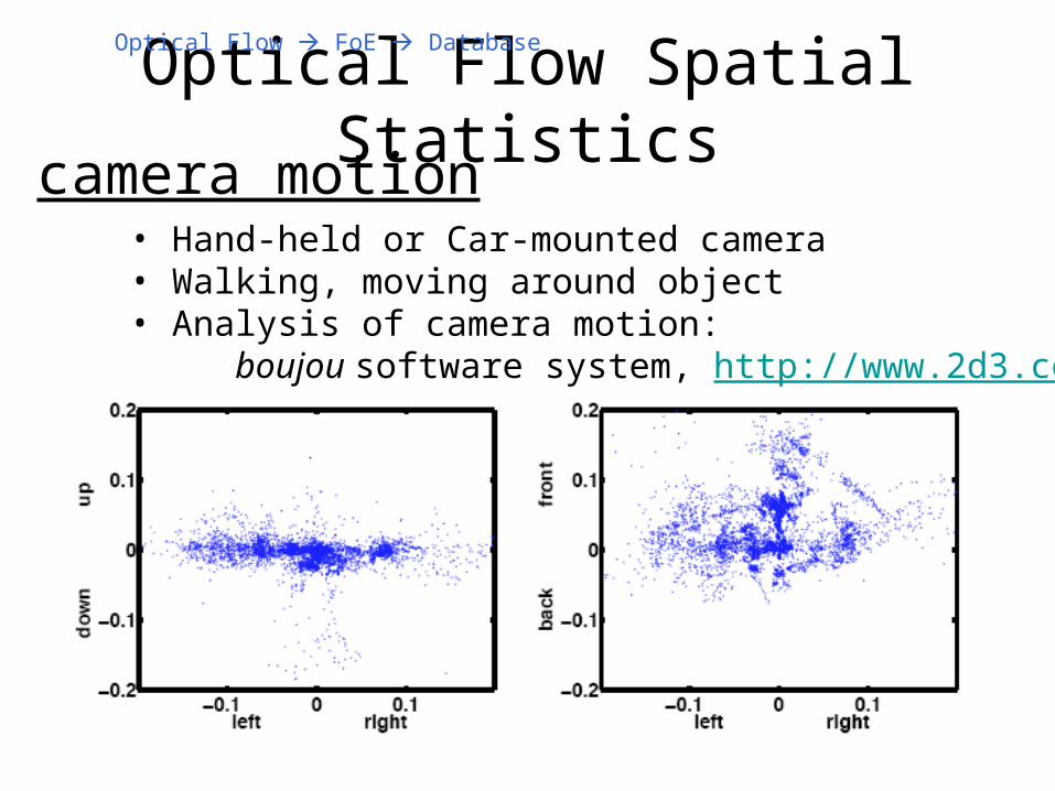
Optical Flow Spatial Statistics
• Hand-held or Car-mounted camera• Walking, moving around object• Analysis of camera motion:
boujou software system, http://www.2d3.com
camera motion
Optical Flow FoE Database

Optical Flow Database generation
The optical flow is simply given by the difference in image coordinates under which a scene point is viewed in each of the two cameras.
Optical Flow FoE Database
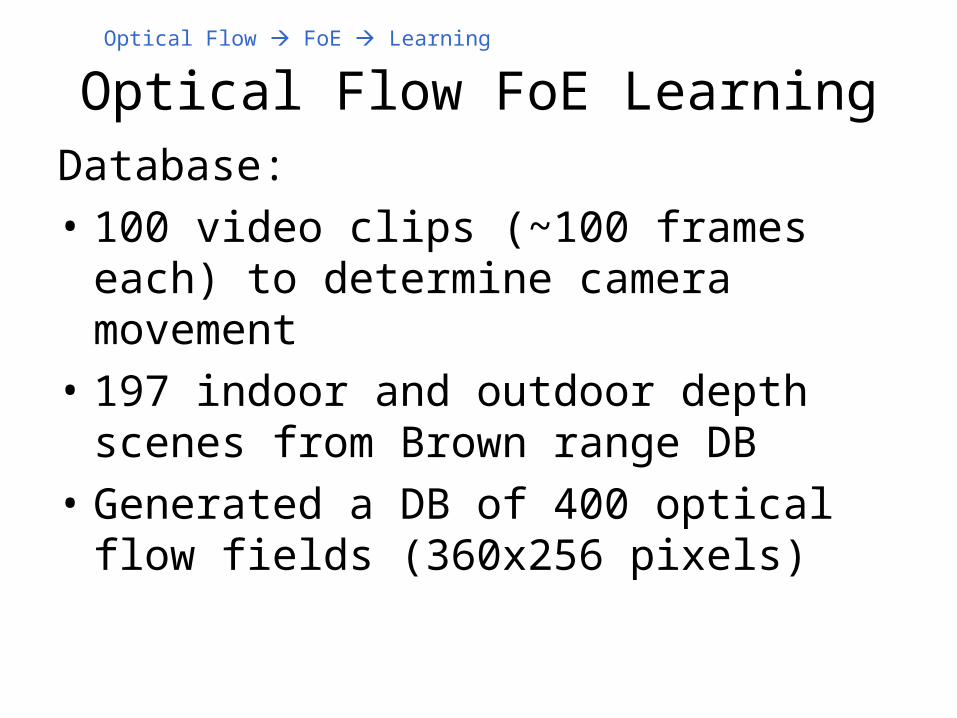
Optical Flow FoE LearningDatabase:
• 100 video clips (~100 frames each) to determine camera movement
• 197 indoor and outdoor depth scenes from Brown range DB
• Generated a DB of 400 optical flow fields (360x256 pixels)
Optical Flow FoE Learning
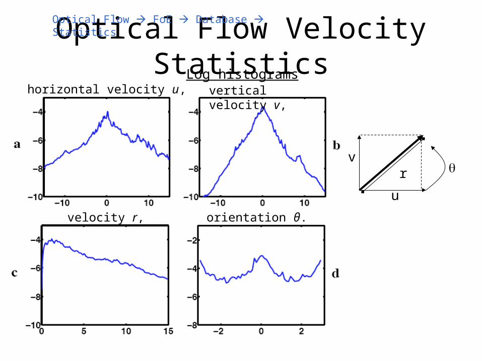
Optical Flow Velocity Statisticshorizontal velocity u, vertical velocity v,
velocity r, orientation θ.
Optical Flow FoE Database Statistics
Log histograms
r
u
v
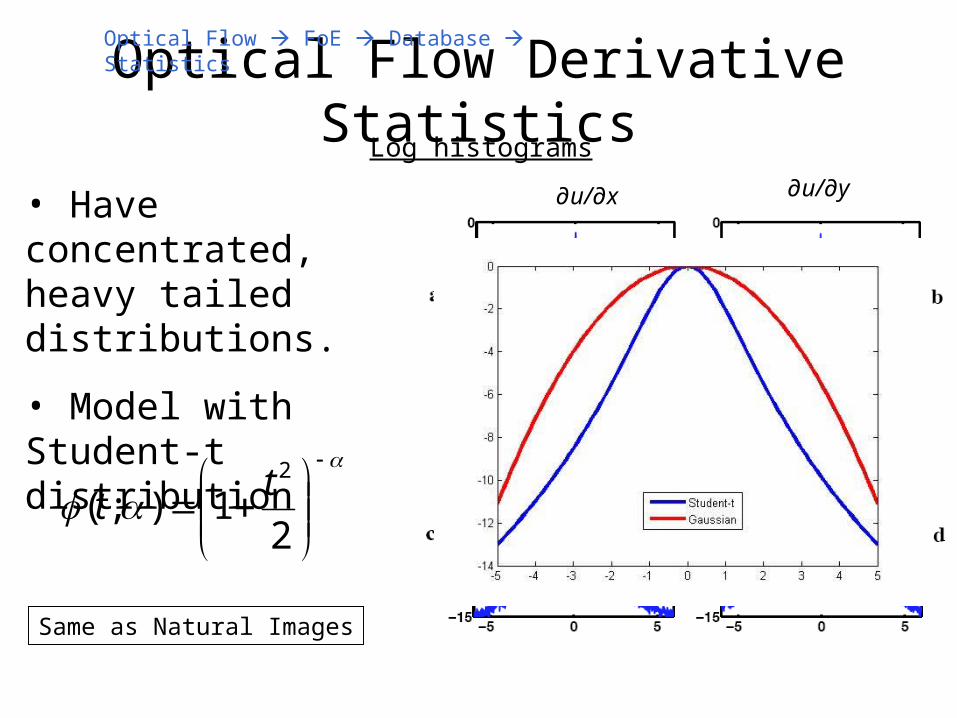
Optical Flow Derivative Statistics
∂u/∂x ∂u/∂y
∂v/∂x ∂v/∂y
• Have concentrated, heavy tailed distributions.
• Model with Student-t distribution
21);(
2tt
Same as Natural Images
Optical Flow FoE Database Statistics
Log histograms

Learning Optical Flow
• MRF of 3x3 or 5x5 cliques– Larger neighborhood than previous works
5x5
3x3
Optical Flow FoE Learning
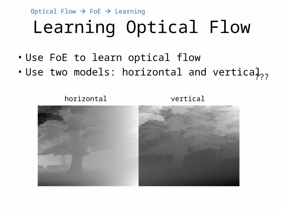
Learning Optical Flow
• Use FoE to learn optical flow
• Use two models: horizontal and vertical
horizontal vertical
Optical Flow FoE Learning
???
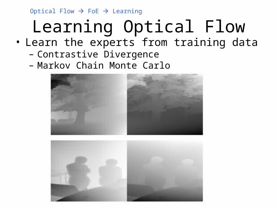
Learning Optical Flow• Learn the experts from training data
– Contrastive Divergence– Markov Chain Monte Carlo
Optical Flow FoE Learning
Optical Flow Evaluation
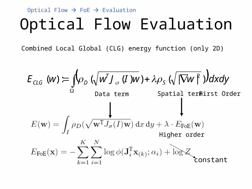
Combined Local Global (CLG) energy function (only 2D)
Data term Spatial term First Order
Higher order
dxdywwIJwwE ST
DCLG )||())((:)( 2
Optical Flow FoE Evaluation
constant
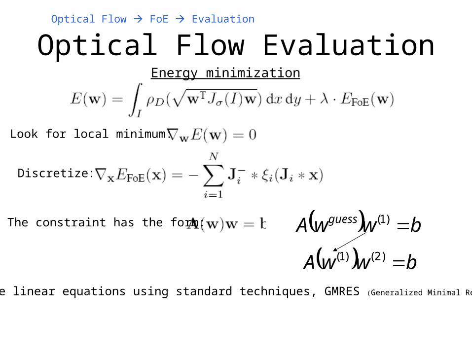
Optical Flow Evaluation
bwwA guess
Look for local minimum:
Discretize:
The constraint has the form:
Solve linear equations using standard techniques, GMRES (Generalized Minimal Residual ).
Optical Flow FoE Evaluation
bwwA )2()1(
bwwA guess )1(
Energy minimization
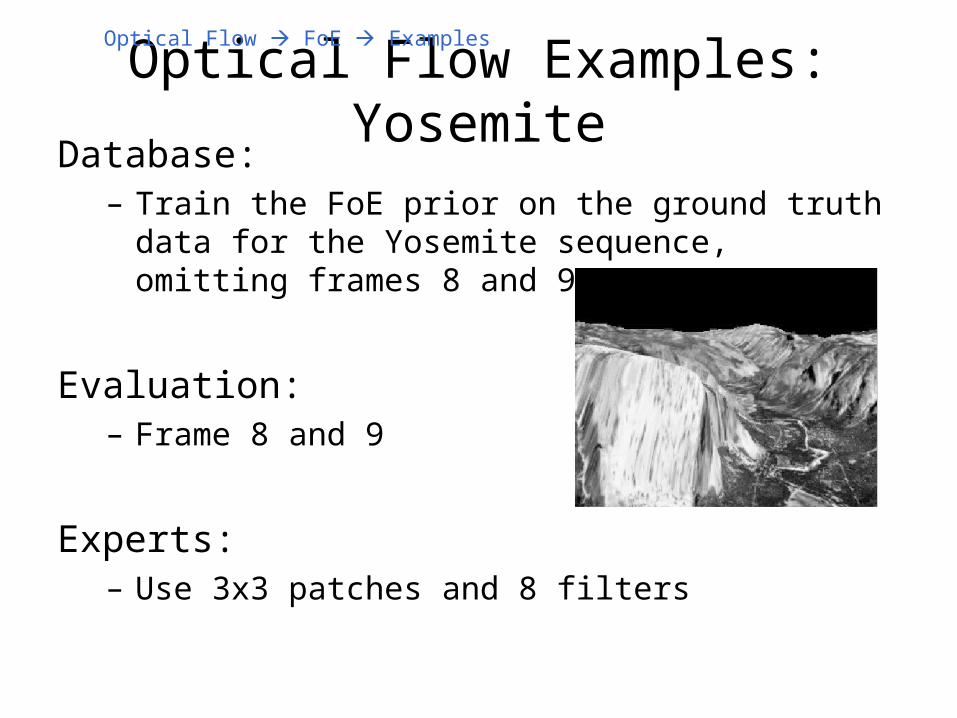
Optical Flow Examples: YosemiteDatabase:
– Train the FoE prior on the ground truth data for the Yosemite sequence, omitting frames 8 and 9
Evaluation:– Frame 8 and 9
Experts:– Use 3x3 patches and 8 filters
Optical Flow FoE Examples

u
v
Optical Flow Examples: YosemiteOptical Flow FoE Examples
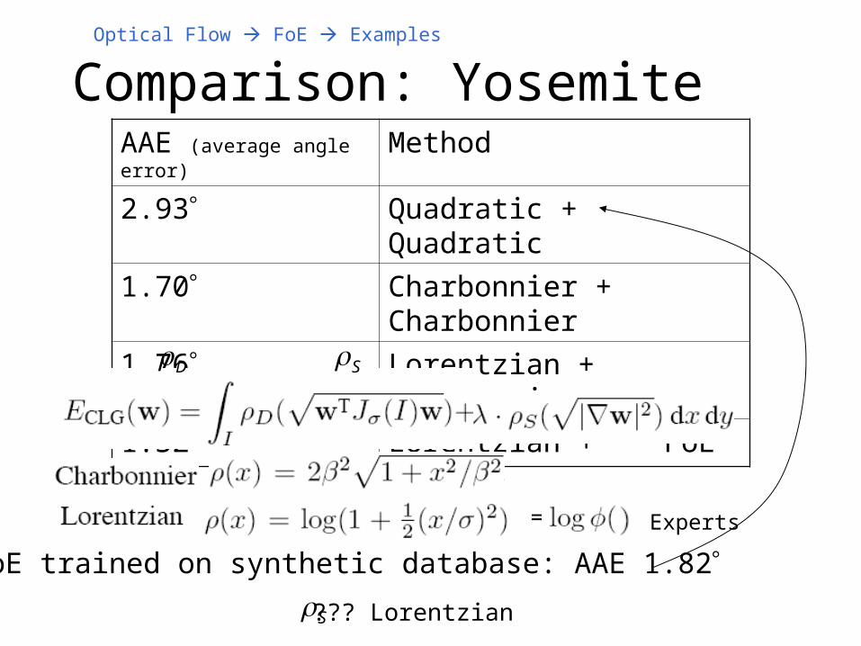
MethodAAE (average angle error)
Quadratic + Quadratic2.93
Charbonnier + Charbonnier1.70Lorentzian + Charbonnier1.76
Lorentzian + FoE1.32
Comparison: Yosemite
Experts=
FoE trained on synthetic database: AAE 1.82
Optical Flow FoE Examples
SD
S Lorentzian???

u
v
Optical Flow Examples: Flower GardenOptical Flow FoE Examples
Remarks:• Initial results of a promising technique:
– Generalization to U\V
– Improved optical flow database
– Include 3D data term
– 5x5 cliques can give better results (?)
Summary
• Field of Experts is a combination of MRF and PoE
• Field of Experts can learn spatial dependence of optical flow sequences
• In contrast to other methods, the FoE prior does not require any tuning of parameters besides
• Combining FoE with CLG gives best results• Given more general training data, generalization
can be improved
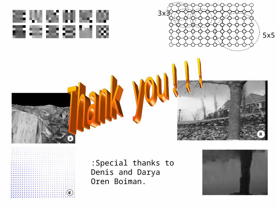
5x5
3x3
Special thanks to:Denis and DaryaOren Boiman.