Learning Parallel Portfolios of Algorithms

Marek Petrik and Shlomo ZilbersteinDepartment of Computer Science

University of Massachusetts Amherst, MA 01003{petrik,shlomo}@cs.umass.edu

April 16, 2007

Abstract

A wide range of combinatorial optimization algorithms have been developed forcomplex reasoning tasks. Frequently, no single algorithm outperforms all the others.This has raised interest in leveraging the performance of a collection of algorithms toimprove performance. We show how to accomplish this using a Parallel Portfolio ofAlgorithms (PPA). A PPA is a collection of diverse algorithms for solving a singleproblem, all running concurrently on a single processor until a solution is produced.The performance of the portfolio may be controlled by assigning different shares ofprocessor time to each algorithm. We present an effective method for finding a PPAin which the share of processor time allocated to each algorithm is fixed. Finding theoptimal static schedule is shown to be an NP-complete problem for a general classof utility functions. We present bounds on the performance of the PPA over randominstances and evaluate the performance empirically on a collection of 23 state-of-the-art SAT algorithms. The results show significant performance gains over the fastestindividual algorithm in the collection.

Keywords: algorithm portfolios, resource bounded reasoning, combinatorial optimiza-tion

1 Introduction

Research advances in search and automated reasoning techniques have produced a widerange of different algorithms for hard decision problems. In most cases, there is no singlealgorithm that is superior to all others on all instances. A good example is satisfiabil-ity (SAT), for which many algorithms have been developed, with no single algorithm thatdominates the performance of all the others. SAT is particularly interesting because it isnot representing a single application; it is a prominent problem in both theoretical and

1

−10,000 −5,000 0 5,000 10,0000

5

10

15

20

25

τa − τ

b

Inst

ance

s

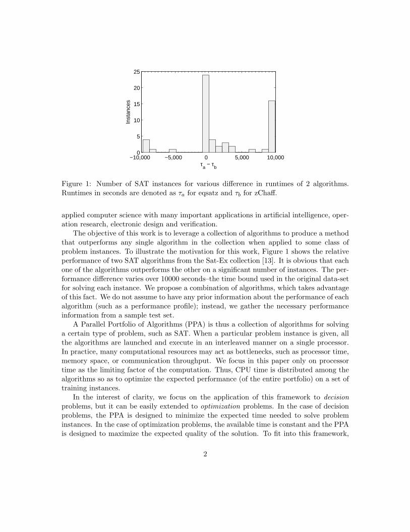
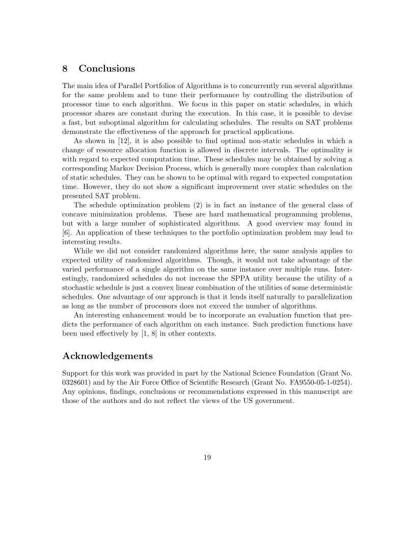
Figure 1: Number of SAT instances for various difference in runtimes of 2 algorithms.Runtimes in seconds are denoted as τa for eqsatz and τb for zChaff.

applied computer science with many important applications in artificial intelligence, oper-ation research, electronic design and verification.

The objective of this work is to leverage a collection of algorithms to produce a methodthat outperforms any single algorithm in the collection when applied to some class ofproblem instances. To illustrate the motivation for this work, Figure 1 shows the relativeperformance of two SAT algorithms from the Sat-Ex collection [13]. It is obvious that eachone of the algorithms outperforms the other on a significant number of instances. The per-formance difference varies over 10000 seconds–the time bound used in the original data-setfor solving each instance. We propose a combination of algorithms, which takes advantageof this fact. We do not assume to have any prior information about the performance of eachalgorithm (such as a performance profile); instead, we gather the necessary performanceinformation from a sample test set.

A Parallel Portfolio of Algorithms (PPA) is thus a collection of algorithms for solvinga certain type of problem, such as SAT. When a particular problem instance is given, allthe algorithms are launched and execute in an interleaved manner on a single processor.In practice, many computational resources may act as bottlenecks, such as processor time,memory space, or communication throughput. We focus in this paper only on processortime as the limiting factor of the computation. Thus, CPU time is distributed among thealgorithms so as to optimize the expected performance (of the entire portfolio) on a set oftraining instances.

In the interest of clarity, we focus on the application of this framework to decisionproblems, but it can be easily extended to optimization problems. In the case of decisionproblems, the PPA is designed to minimize the expected time needed to solve probleminstances. In the case of optimization problems, the available time is constant and the PPAis designed to maximize the expected quality of the solution. To fit into this framework,

2

the individual algorithms must be preemptable without a significant overhead (i.e., it isassumed that they can be stopped and resumed with negligible overhead). Furthermore,optimization algorithms must have the anytime property [3, 14]. Anytime algorithms maybe interrupted before their termination and return an approximate solution. The qualityof the solution typically improves with computation time.

Prior knowledge of the algorithms’ performance on instances may enhance the perfor-mance of a portfolio by always using the most suitable algorithm for each instance. But itis usually impossible to have perfect prior knowledge without actually solving the instance.However, there have been some research efforts to estimate the performance by the similar-ity of the input instance to instances with known performance. This way, easily-computablefeatures of the problem instance may help to approximately determine the performance ofeach algorithm on that instance. Finding informative features that always enhance theprediction of performance is a hard problem. It is generally known as algorithm portfolioselection [5, 8].

In related work, Gomes and Selman [5] provide an empirical evaluation of composingrandomized search algorithms on multiple processors into portfolios. Their results indicatethat it may be beneficial to combine randomized algorithms with high variance and runthem in parallel. For a single processor, they found random restarts to produce verygood results. A successful algorithm portfolio selection approach was also taken by [8].It is based, like many other approaches, on using a training set of problem instancesto estimate a probabilistic model of the performance. Statistical regression is used todetermine the best algorithm for instances of combinatorial auction winner determination.Unlike previous approaches that use experimental methods to determine the compositionof the portfolio, our approach defines a formal model for the problem, and analyzes thetheoretical properties of the model and solution techniques.

The rest of the paper is organized as follows. Section 2 defines the framework used tomodel algorithm portfolios and their performance. In Section 3, we present an algorithmfor finding a locally optimal PPA for a specified set of algorithms. A globally optimalalgorithm and computational complexity bounds are described in Section 4 and Section 5.The following section, Section 6, presents basic theoretical generalization bounds of the ap-proach. Finally, in Section 7 we demonstrate the effectiveness of this approach by applyingit to a collection of 23 state-of-the-art Satisfiability (SAT) algorithms.

2 Framework

In this section we develop a general framework for creating parallel portfolios of algorithms.As indicated above, we develop the framework specifically for decision algorithms, but theextension to optimization algorithms is straightforward. We mention briefly the necessarymodifications throughout the paper.

A problem domain is a set of all possible problem instances together with a probability

3

distribution over them, denoted as X . The probability distribution of encountering theinstances is stationary. An algorithm is a function that maps an input problem instanceto a solution. Notice that the algorithms are assumed to be deterministic.

To preserve flexibility of the framework, we use the notion of utility that correspondsto the performance of an algorithm on an instance. For standard decision algorithms, itdepends on the computation time; for optimization algorithms, it depends on the qualityof the solution within a certain amount of time. Thus the utility function is defined asu : X → R. The PPA performance will be optimized with respect to a training set I ofinstances, randomly drawn from the domain X . The following definitions assume instancesfrom the set X , which may be extremely large or infinite. However, the proposed scheduleoptimization algorithms optimize the portfolio with regard to utility on the training set I.

The performance of a PPA depends on the processor share that is assigned to eachalgorithm. The share assigned to an algorithm at each point of time is determined byits resource allocation function, as defined below. Resource allocation functions for allalgorithms in the portfolio comprise the schedule. In this paper we consider only constantallocation functions, but they can be extended to a wider class of functions, as shownin [12].

Definition 2.1. The resource allocation function (RAF) for an algorithm a is a constantfrom the interval [0, 1] that defines its share of the processor time.

We now extend the notion of utility to be determined not only by an algorithm and aninstance, but also by its resource allocation function. The precise function depends on theactual algorithm.

Definition 2.2. The resource utility function of algorithm a is: ua : [0, 1]×X → R.

Definition 2.3. A Static Parallel Portfolio of Algorithms (SPPA) P is a tuple (A, s),where A is a finite list of algorithms with resource utility functions and s is a schedule,that is a vector of resource allocations for algorithms from A.

The resource allocation to the jth algorithm of the portfolio is denoted as s[j]. Theresource allocations must fulfill the resource limitation constraint, so the set of allowedschedules is S = {s

∑nj=1 s[j] ≤ 1}.

In the following, m = |I| and n = |A|. An intrinsic characteristic of PPAs is that onlyone result for a problem instance may be used, even if more algorithms provide solutions.Therefore, the PPA utility of an instance is the maximal utility of all individual algorithms.This is in contrast with ensemble learning, where classifiers vote and the ensemble resultis the average of the votes.

Definition 2.4. The utility U(s, x) of a PPA is the maximum utility that any algorithmof the portfolio achieves on instance x ∈ X using schedule s ∈ S, that is:

U(s, x) = maxj=1,...,n

uj(s[j], x).

4

We denote the average performance of the schedule on the training set instances as

U(s) =1m

m∑i=1

U(s, xi).

Then the problem of selecting the best schedule is defined as

s = arg maxs∈S

U(s).

Some additional measures of performance are proposed in [12].The definition of the utility of an algorithm with respect to a problem instance depends

on the specific problem setting. For decision problems, the available time is unlimited, butit is preferable to have a PPA that solves the problems as fast as possible. Assuming thealgorithms may be executed on a single processor with no overhead, the utility function isdefined as follows.

Definition 2.5. For decision algorithms, the time to find the first solution is optimized ifthe resource utility function u for an algorithm is

u(r, x) = −τx

r,

where τx is the time to solve the instance x and r is the resource allocation function. Thefunction u is concave and twice continuously differentiable in r.

To apply the framework to optimization problems, we may assume that the computationtime is fixed and the quality of the obtained solutions is important. Anytime algorithmscan be characterized by their performance profile function f that maps the computationtime to the current solution quality. Let T be the time allocated for the execution of thePPA. Then, the resource utility function that maximizes the obtained quality is

u(r, x) = f(T ∗ r, x).

3 The Classification-Maximization Algorithm

In this section we present an algorithm to find locally optimal schedules for SPPAs. Thetask of finding the optimal static schedule on I may be formulated as the following non-linear mathematical optimization problem:

maximize U(s) =m∑

i=1

maxj=1,...,n

uj(s[j], xi)

subject ton∑

j=1

s[j] = 1,

s[j] ≥ 0 j = 1, . . . , n

(1)

5

This problem is not solvable by standard non-linear programming techniques because theinner max operator makes the objective function discontinuous. To solve the program, wepropose to decompose the solution process into two phases: classification and maximization.Hence the Classification-Maximization Algorithm.

The algorithm is based on a reformulation of (1) that removes the inner maximization.In order to do this, we introduce a classification matrix W = m × n. Notice that we donot assume W to be given, but it represents additional optimization variables. Intuitively,the entries of the matrix indicate the best algorithm for each problem instance. In otherwords, the entry Wij = 1 if and only if algorithm j has the highest utility for instance i,given the resource allocation. Clearly, for each instance exactly one algorithm is optimal,breaking ties arbitrarily. Therefore, the matrix must fulfill:

n∑j=1

Wij = 1 i = 1, . . . ,m.

Using the matrix W , we can divide the set of instances I into subsets Ij , j = 1, . . . , naccording to which algorithm the instance is assigned. Formally, we can write

Ij = {xi Wij = 1} ,

with the cardinality of these sets denoted as mj = |Ij |.To simplify the notation, we introduce a classification function k(l, j), which denotes

the index of the l-th instance from Ij . Formally, it is defined as the minimal i′ that satisfies∑i′

i=1 Wij = l.Using a classification matrix W , the problem may be reformulated as

maximize U(s,W ) =m∑

i=1

n∑j=1

Wijuj(s[j], xi)

subject ton∑

j=1

s[j] = 1,

n∑j=1

Wij = 1 i = 1, . . . ,m,

s[j] ≥ 0 j = 1, . . . , n,

Wij ∈ {0, 1} i = 1, . . . ,m

j = 1, . . . , n

(2)

To illustrate the possible values of W , consider a simple example with two algorithmsa1 and a2, and three instances x1, x2, and x3. Assume that the result of the optimization

6

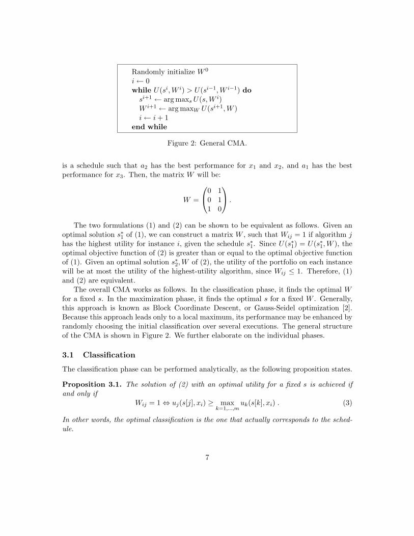
Randomly initialize W 0

i← 0while U(si,W i) > U(si−1,W i−1) do

si+1 ← arg maxs U(s,W i)W i+1 ← arg maxW U(si+1,W )i← i + 1

end while

Figure 2: General CMA.

is a schedule such that a2 has the best performance for x1 and x2, and a1 has the bestperformance for x3. Then, the matrix W will be:

W =

0 10 11 0

.

The two formulations (1) and (2) can be shown to be equivalent as follows. Given anoptimal solution s∗1 of (1), we can construct a matrix W , such that Wij = 1 if algorithm jhas the highest utility for instance i, given the schedule s∗1. Since U(s∗1) = U(s∗1,W ), theoptimal objective function of (2) is greater than or equal to the optimal objective functionof (1). Given an optimal solution s∗2,W of (2), the utility of the portfolio on each instancewill be at most the utility of the highest-utility algorithm, since Wij ≤ 1. Therefore, (1)and (2) are equivalent.

The overall CMA works as follows. In the classification phase, it finds the optimal Wfor a fixed s. In the maximization phase, it finds the optimal s for a fixed W . Generally,this approach is known as Block Coordinate Descent, or Gauss-Seidel optimization [2].Because this approach leads only to a local maximum, its performance may be enhanced byrandomly choosing the initial classification over several executions. The general structureof the CMA is shown in Figure 2. We further elaborate on the individual phases.

3.1 Classification

The classification phase can be performed analytically, as the following proposition states.

Proposition 3.1. The solution of (2) with an optimal utility for a fixed s is achieved ifand only if

Wij = 1⇔ uj(s[j], xi) ≥ maxk=1,...,m

uk(s[k], xi) . (3)

In other words, the optimal classification is the one that actually corresponds to the sched-ule.

7

Proof. The proof of necessary optimality condition is by contradiction. Assume that theoptimal solution does not satisfy (3). So let Wij = 1, be a classification with a suboptimalutility. Let j∗ = arg maxj=1,...,m uj(s[j], xi), breaking ties arbitrarily. Clearly, settingWij = 0 and Wij∗ = 1 does not invalidate the classification constraints. Since this holdsfor all i, the monotonicity of

∑implies that the utility is not decreased. Therefore, the

solution that fulfills the condition must also have the optimal utility. The proof of sufficientoptimality condition is similar.

3.2 Maximization

For the maximization phase, we need the following assumption on the resource utilityfunctions.

Definition 3.2. A set A of resource utility functions uj is homogeneous if each utilityfunction can be expressed as

uj(r, x) = ρj(r) ∗ ηj(x).

Notice that the resource utility functions are homogeneous for decision algorithms. Ifthe resource utility functions are homogeneous then the maximization phase is equivalentto solving

maximize U(s) =n∑

j=1

ρj(s[j])mj∑i=1

ηj(xk(l,j))

subject ton∑

j=1

s[j] = 1

s[j] ≥ 0 j = 1, . . . , n

(4)

Let dj =∑mj

i=1 ηj(xk(i,j)). The problem then becomes the following.

maximize U(s) =1m

n∑j=1

ρj(s[j])dj

subject ton∑

j=1

s[j] = 1

s[j] ≥ 0 j = 1, . . . , n

(5)

This is easily solved by first order necessary conditions, and from the fact that the probleminvolves a maximization of a concave function on a convex set. Hence the following theorem.

Theorem 3.3. The solution of (5) is globally optimal if it fulfills

ρ′j(s[j])ρ′k(s[k])

=dk

dj.

8

Proof. The Lagrangian function of (5) is

L(s, λ) = − 1m

n∑j=1

ρj(s[j])dj + λn∑

j=1

s[j].

The theorem then follows from the second order optimality conditions [2]. Because theof the schedulability assumption, it also fulfills the convexity criterion. Thus this localmaximum is also global.

The theorems above complete the definition of CMA. In general, CMA is a suboptimalalgorithm.

3.3 Decision Problems

For decision problems with no switching overhead, the utility function is formulated ac-cording to Definition 2.5. Thus we have that:

ρj(r) =1rηj(x) = τj(x).

Now the maximization phase of the CMA can be solved as the following theorem states.

Theorem 3.4. Let the SPPA use decision algorithms. The mean optimal schedule for themaximization phase of CMA, given a fixed classification, must fulfill

s[o]s[p]

=

√∑moi=1 τo(xk(i,o))∑mp

i=1 τp(xk(i,p)).

Proof. By Theorem 3.3.

Theorem 3.5. Let s be the optimal schedule of a PPA for decision problems, obtained inthe maximization phase of CMA for mean optimization. Then the expected execution timeof the schedule is n∑

j=1

√√√√ 1m

mj∑i=1

τj(xk(i,j))

2

.

Proof. The theorem follows directly from Theorem 3.4.

9

4 Optimal Algorithm

It is possible to find an optimal static schedule by searching for the optimal schedule for ev-ery possible classification. This approach leads to the optimal solution because the locallyoptimal schedule for the optimal classification is also globally optimal. The computationalcomplexity of this approach is very high because the number of these classifications is expo-nential in the number of instances. However, not all of the classifications are possible whenactually running the portfolio. For example, it is possible that if algorithm a1 outperformsalgorithm a2 on instance x2 then it also outperforms it on x1. Thus, a classification thatassigns x2 to a1 and x1 to a2 cannot happen during a real execution of a PPA. When weassume that the algorithms in the portfolio have homogeneous utility functions, we canlimit the number of all realistic classifications to be polynomial in the number of instancesand exponential in the number of algorithms as we show this section. The results fromthis section also help to establish the generalization bounds in Section 6.

Definition 4.1. A classification is valid when there exists a schedule that exactly definesit.

It is clear from Lemma 3.1 that for any classification that is not valid there is a validclassification with better or equal performance. Thus, limiting the search to valid classifi-cations is sufficient to guarantee that an optimal schedule will be found.

Lemma 4.2. Let s∗ be the globally optimal schedule of a PPA and let s be the best scheduleobtained from a valid classification and a single maximization phase. Then

U(s∗) = U(s).

Proof. We show that the lemma holds by contradiction. Let

U(s∗) > U(s).

Clearly, a classification W ∗ defined by schedule s∗ is valid. Then, by running the maxi-mization phase of CMA on this classification, we get a schedule s′. Then, we get

U(s′) ≥ U(s∗) > U(s),

which contradicts the optimality condition of s.

The set of valid schedules depends on the properties of the resource utility functions.In particular, we focus on the homogeneity of the functions. The main reason is that theresource utility functions of decision algorithms are homogeneous.

Lemma 4.3. Let the resource utility function be homogeneous. Let a, b be arbitrary algo-rithms from a PPA. Then, for any valid classification Ia, Ib, we have

xo ∈ Ia ∧ xp ∈ Ib ⇒ηa(xo)ηb(xo)

≥ ηa(xp)ηb(xp)

,

where Ia is the set of instances assigned to a and Ib to b.

10

Notice that this lemma is applicable also for the case of more than two algorithms.Then, Ia ∪ Ib ⊂ I, i.e., Ia ∪ Ib is a proper subset of I.

Proof. Because the classification is valid,

ua(xo) ≥ ub(xo)ua(xp) ≥ ub(xp).

¿From the homogeneity assumption, we get that

ηa(xo)ρa(ra) ≥ ηb(xo)ρb(rb)ηa(xp)ρa(ra) ≤ ηb(xp)ρb(rb).

Hence

ρb(rb)ρa(ra)

≤ ηa(xo)ηb(xo)

ρb(rb)ρa(ra)

≥ ηa(xp)ηb(xp)

,

and the lemma follows.

As a consequence, we have the following lemma.

Lemma 4.4. Let the resource utility functions be homogeneous. For any two instancesxo, xp, and algorithms a and b, without loss of the generality

ηa(xo)ηb(xo)

>ηa(xp)ηb(xp)

.

Then for a valid classification

(xo ∈ Ib ⇒ xp /∈ Ia) ∧ (xp ∈ Ia ⇒ xo /∈ Ib) ,

where Ia is the set of instances assigned to a and Ib to b.

Proof. To show xo ∈ Ib ⇒ xp /∈ Ia by contradiction, assume

xo ∈ Ib ∧ xp ∈ Ia.

Then, application of Lemma 4.3 leads to

ηa(xo)ηb(xo)

≤ ηa(xp)ηb(xp)

,

what is clearly a contradiction. The other statement, xp ∈ Ia ⇒ xo /∈ Ib, can be provedanalogously.

11

i = 0U∗ = 0Initialize split points (p1, . . . , p(n

2)) = (0, . . . , 0)

for all (p1, . . . , p(n2)

) ∈ (0 . . .m)(n2) do

Create W from p1, . . . , p(n2)

)if W is valid then

U ← maxs U(s,W )U∗ ← max{U,U∗}

end ifend for

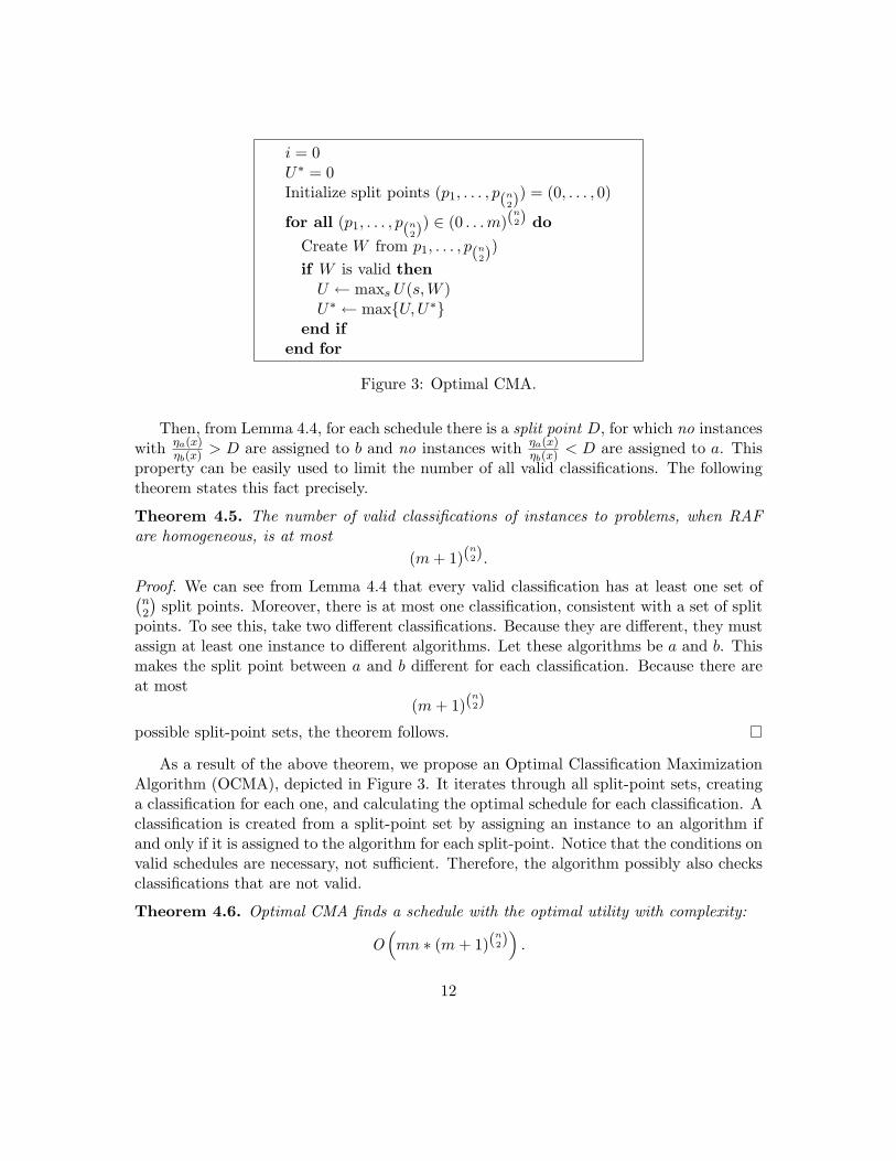
Figure 3: Optimal CMA.

Then, from Lemma 4.4, for each schedule there is a split point D, for which no instanceswith ηa(x)

ηb(x) > D are assigned to b and no instances with ηa(x)ηb(x) < D are assigned to a. This

property can be easily used to limit the number of all valid classifications. The followingtheorem states this fact precisely.

Theorem 4.5. The number of valid classifications of instances to problems, when RAFare homogeneous, is at most

(m + 1)(n2).

Proof. We can see from Lemma 4.4 that every valid classification has at least one set of(n2

)split points. Moreover, there is at most one classification, consistent with a set of split

points. To see this, take two different classifications. Because they are different, they mustassign at least one instance to different algorithms. Let these algorithms be a and b. Thismakes the split point between a and b different for each classification. Because there areat most

(m + 1)(n2)

possible split-point sets, the theorem follows.

As a result of the above theorem, we propose an Optimal Classification MaximizationAlgorithm (OCMA), depicted in Figure 3. It iterates through all split-point sets, creatinga classification for each one, and calculating the optimal schedule for each classification. Aclassification is created from a split-point set by assigning an instance to an algorithm ifand only if it is assigned to the algorithm for each split-point. Notice that the conditions onvalid schedules are necessary, not sufficient. Therefore, the algorithm possibly also checksclassifications that are not valid.

Theorem 4.6. Optimal CMA finds a schedule with the optimal utility with complexity:

O(mn ∗ (m + 1)(

n2))

.

12

Proof. The utility is optimal because each valid schedule has a unique split-point set byLemma 4.4, and it is sufficient to enumerate all valid schedules by Lemma 4.2. Thecomplexity is evident from the total number of split-point sets and Theorem 3.3.

¿From the above analysis we have an algorithm that is polynomial in the number ofinstances and exponential in the number of algorithms. Moreover, the OCMA enumeratesalso classifications that are not valid. Thus it is questionable whether the exponentialcomplexity of the OCMA is caused by its inefficient enumeration or whether the number ofvalid classifications is exponential. We show, to address this issue, that simply enumeratingall valid classifications cannot lead to a polynomial algorithm, and later in Section 5, wealso show that the general problem of finding the optimal schedule for a set of homogeneousalgorithms is NP-hard.

Proposition 4.7. The number of valid classifications may be exponential in the descriptionof the problem, even when using decision algorithms.

Proof. To prove the proposition, we show an example with an exponential number of validclassification. We construct a scheduling instance with n + 1 algorithms and n instancesfor any n. Let the algorithms be A = {a0 . . . an} and instances X = {x1 . . . xn}. Sincewe are dealing with decision algorithms, the utility on the instances is determined by thesolution time τa(x) on each instance x. We define these solution times as follows:

τ0(xi) = 1 i = 1, . . . , n

τi(xi) = 1 i = 1, . . . , n

τj(xi) = 2 i, j = 1, . . . , n and i 6= j

Now we show that any classification of instances to algorithm a1 is possible, thus creatingat least 2i distinct classifications. Let σ(xi) be the indicator function whether xi is assignedto algorithm a0. For arbitrary σ, we can define schedule s as follows to achieve the properinstance assignment:

s[0] = ε′ ∗ 1n + 1

s[j] = ε ∗ 1n + 1

σ(j) = 0

s[j] = φ ∗ 1n + 1

σ(j) = 1,

where

φ < ε′ < ε < 2ε′

ε′ + (n− |σ|) ∗ ε + |σ| ∗ φ = n + 1.

13

Such ε, ε′, and φ always exist and the conditions ensure that the schedule sums to 1. Theclassification of this schedule clearly satisfies σ, since:

σ(xi) = 1 ⇒ τ0(xi)s[0]

=n + 1

ε′<

n + 1φ

=τi(xi)s[i]

σ(xi) = 1 ⇒ τ0(xi)s[0]

=n + 1

ε′<

n + 1ε2

=2(n + 1)

ε=

τj(xi)s[j]

σ(xi) = 0 ⇒ τ0(xi)s[0]

=n + 1

ε′>

n + 1ε

=τi(xi)s[i]

.

As a result, just enumerating the valid schedules cannot lead to a polynomial algorithm.Thus, the exponential complexity of the OCMA cannot be resolved by a better enumerationof valid schedules.

5 Complexity Analysis

This section describes the complexity analysis of the SPPA scheduling problem. Specifi-cally, the SPPA scheduling problem is the question whether there is a schedule s such thatU(s) ≥ K. We show that this problem is NP hard.

Definition 5.1. In a 0-1 knapsack problem a set of positive integer pairs {(ci, wi) i =1, . . . , N} is given. The problem is whether there exists a subset T such that

∑i∈T ci ≥ C

and∑

i∈T wi ≤W .

The 0-1 knapsack problem is NP complete [10, 11]. We assume below that a descriptionof the utility function is included in the scheduling problem.

Theorem 5.2. The scheduling problem is NP-hard even for homogeneous utility functions.

The proof of this theorem may be found in Appendix A.1.We proved NP-hardness for the problem of finding schedules for algorithm with general

resource utility functions. While this result is not directly applicable to decision algo-rithms, it indicates that homogeneity of the resource utility functions is not sufficient tomake the problem easier. The main difficulty in complexity analysis of scheduling decisionalgorithms is that it is not a combinatorial problem, because their resource utility functionsare continuous.

6 Theoretical Generalization Bounds

This section describes the generalization properties of the SPPA approach. Since theschedules are based on a training set of instances, it is important to be able to predict

14

how well the SPPA may perform on X , the domain of all problem instances. We proveonly the worst case bounds.These bounds have mostly theoretical significance as they showinteresting asymptotic generalization behavior. The bounds in this section are motivatedby the Probably Approximately Correct (PAC) learning framework [9].

The main goal is to show that the number of training instances required to learn anSPPA that performs well on all instances is reasonably small. Because training instancesare drawn randomly, the bounds only hold with a certain probability. Note that thebounds apply to the meta-level scheduling algorithm, such as CMA, that optimizes theSPPA schedule.

In this section, we assume that all SPPAs we refer to are composed of the same setof algorithms; they only differ in the actual schedules. Notice that since an SPPA alsocontains the schedule, it behaves just as a simple algorithm. Thus, the utility of an SPPAon the training set is its empirical mean utility, defined as:

Um(s) =1m

m∑i=1

U(s,Xi),

where Xi is a random variable, representing an instance randomly drawn from X . Noticethat Um(s) is a random variable.

We define two properties of SPPAs, generalization and optimality. An SPPA learningalgorithm generalizes well, when the utility on all instances is close to the utility on thetraining set. An SPPA learning algorithm is optimal, if the optimal SPPA on the trainingset is close to the optimal result on the set of all instances. These properties are formalizedby the following definition.

Definition 6.1. We say that an SPPA learning algorithm mean-generalizes, if for any0 < ε and 0 < δ < 1 it outputs an SPPA s ∈ S, for which

P [Um(s)−E [U(s,X)] > ε] ≤ δ.

Let the globally optimal algorithm be:

s∗ = arg maxs∈S

E [U(s,X)] .

We say that an SPPA learning algorithm is mean optimal, if for all 0 < ε and 0 < δ < 1 itoutputs a schedule s

P [E [U(s∗, X)]−E [U(s,X)] > ε] ≤ δ.

In both cases, the learner must use at most a polynomial number of training instances in1δ and 1

ε to achieve the bound.

The following theorem probabilistically bounds the expected performance of an SPPAon a sample of size m.

15

Theorem 6.2. Let the resource utility functions be homogeneous. Let u, η, ρ be themaximal values of corresponding functions for the given set of algorithms. In addition, letm∗ε2u2 > 2. Then, the generalization probability is

P[sups∈S|Um(s)−E [U(s,X)] | > ε

]≤ 8(m + 1)(

n2)2n exp

(−mε2

32u

(1

ρηn

)2)

.

The proof of this theorem is quite technical and it is in Appendix A.2.

Theorem 6.3. Let the assumptions of Theorem 6.2 hold. Also let

z = (ρηn)2u.

An algorithm that finds a static schedule by maximizing the empirical mean utility will findthe ε mean optimal SPPA with probability at least 1− δ using at most

max

(512(n2

)z

ε2ln

256(n2

)z

ε2,256z

ε2ln

2n+3

δ

)

samples.

Proof. The proof is based on Problem 12.5 from [4]. Let

d =ε2

u

(1

ρηn

)2

.

Further, whenever m ≥ 512(n2)

d ln256(n

2)d we have the following bound

(m + 1)(n2) ≤ exp

(md

256

).

The theorem follows straight forward from the bound.

Remark 6.4. A tighter bound could be obtained using Vapnik-Chervonenkis results thatassume that the training set can be learned with zero training error, as in Section 12.7of [4].

16

a E [u(I)] Var [u(I)] E [u(IS)] Var [u(IS)]

zChaff 372.3 2633.3 251.1 2140.2relsat 715.0 3599.2 595.9 3274.3relsat 951.0 4198.5 833.4 3934.4sato 994.4 4103.7 877.0 3833.7

SPPA 233.2 2005.6 77.1 1000.5

Table 1: Results of a few best-performing algorithms from Sat-Ex and the best SPPA after200 runs of CMA.

7 Application

We examined the applicability of the SPPA approach to combining 23 state-of-the-artalgorithms for the satisfiability problem (SAT). The SAT problem is to determine whethera formula in propositional logic is satisfied for at least one interpretation. It offers a generalframework for problem solving and planning [7]. The performance results of the algorithmswere taken from [13]. The results are from runs of the algorithm on 1,303 instances. Thecutoff execution time was 10,000 seconds. For the purpose of evaluation, we used a solutiontime of 20,000 seconds for instances that were not solved within the 10,000-second limitto emulate the possible expected solution time. The choice of this value did not have asignificant impact on the results.

The set of all available instances from [13] is denoted as I. The set of all instancesthat are solvable by at least one available algorithm is denoted as IS . The best performingalgorithm from the group was zChaff, with average execution time 372 seconds on I and251 on IS . The performance of the four fastest algorithms on the set is summarized inTable 1.

We tested CMA for both I and IS . In both cases the CMA-calculated SPPA signif-icantly outperforms the best algorithm for the instance set (zChaff). The performanceof the SPPA was derived analytically from the available performance data of individualalgorithms. In the case of I, the mean execution time was lower by 37%, and the standarddeviation was lower by 24%. In the case of IS , the mean execution time was lower by 68%and the standard deviation was lower by 55%. The impressive results on IS were mainlydue to the fact that each instance is solved by at least one algorithm, thus reducing thevery long runtime for those instances. The results are summarized in Table 1.

Specific schedules that were obtained are shown in Table 2. We used all 23 availablealgorithms for calculating the optimal schedules, but only the listed algorithms had non-zero processor share for the two schedules. It is interesting that though zChaff is the fastestalgorithm, the fraction of processor it uses is very small in both schedules. The intuitiveexplanation is that zChaff is fast on instances that are hard to solve, but for the rest, it is

17

Algorithms P1 P2

eqsatz 0.857 0.104nsat 0.002 0.002ntab-back2 0.030 0.026heerhugo 0.004 0.004satz 0.014 0.739zChaff 0.093 0.125

Performance 233.2 294.8

Table 2: Summary of two SPPAs calculated using CMA with a different starting classifica-tion. P1 is the best SPPA we obtained using CMA. P2 is a locally optimal SPPA obtainedby CMA from a different initialization.

I ′ E [U I ′] E [U I] E [U I ′′] E [u(a) I ′′]

I1 399.8 387.4 359.4 373.2I2 225.1 418.8 856.1 280.4I3 380.1 311.7 268.7 310.9I4 228.5 297.3 340.6 390.5I5 225.2 259.7 281.4 375.0

Table 3: Performance of SPPA U on the training set I and test set I ′′ = I \ I ′. Theschedules were obtained by CMA for I ′. The performance of zChaff, the overall fastestSAT algorithm, is denoted as u(a).

a little slower than some other algorithms.Certainly, the fact that we used the same set for obtaining the optimal SPPA and for

evaluation adds a significant bias toward the method. Nevertheless, it provides a usefuloptimistic limit on the possible gain by using multiple algorithms, which is substantial. Toaddress this issue, we also evaluated the generalization properties experimentally. Unfor-tunately, the small size of the overall instance database limited the significance of theseresults. But we managed to demonstrate the benefit of SPPAs in this case as well. Werandomly choose subsets of all instances and used CMA to find the locally best algorithmfor the set. Then, we evaluated the performance on the set of all algorithms. The instancesets of size 400 were I1 and I2. Instance sets of size 800 were I3, I4, and I5. The results areshown in Table 3. On 4 out of 5 training sets, the best SPPA significantly outperformedzChaff on the test set.

18

8 Conclusions

The main idea of Parallel Portfolios of Algorithms is to concurrently run several algorithmsfor the same problem and to tune their performance by controlling the distribution ofprocessor time to each algorithm. We focus in this paper on static schedules, in whichprocessor shares are constant during the execution. In this case, it is possible to devisea fast, but suboptimal algorithm for calculating schedules. The results on SAT problemsdemonstrate the effectiveness of the approach for practical applications.

As shown in [12], it is also possible to find optimal non-static schedules in which achange of resource allocation function is allowed in discrete intervals. The optimality iswith regard to expected computation time. These schedules may be obtained by solving acorresponding Markov Decision Process, which is generally more complex than calculationof static schedules. They can be shown to be optimal with regard to expected computationtime. However, they do not show a significant improvement over static schedules on thepresented SAT problem.

The schedule optimization problem (2) is in fact an instance of the general class ofconcave minimization problems. These are hard mathematical programming problems,but with a large number of sophisticated algorithms. A good overview may found in[6]. An application of these techniques to the portfolio optimization problem may lead tointeresting results.

While we did not consider randomized algorithms here, the same analysis applies toexpected utility of randomized algorithms. Though, it would not take advantage of thevaried performance of a single algorithm on the same instance over multiple runs. Inter-estingly, randomized schedules do not increase the SPPA utility because the utility of astochastic schedule is just a convex linear combination of the utilities of some deterministicschedules. One advantage of our approach is that it lends itself naturally to parallelizationas long as the number of processors does not exceed the number of algorithms.

An interesting enhancement would be to incorporate an evaluation function that pre-dicts the performance of each algorithm on each instance. Such prediction functions havebeen used effectively by [1, 8] in other contexts.

Acknowledgements

Support for this work was provided in part by the National Science Foundation (Grant No.0328601) and by the Air Force Office of Scientific Research (Grant No. FA9550-05-1-0254).Any opinions, findings, conclusions or recommendations expressed in this manuscript arethose of the authors and do not reflect the views of the US government.

19

References

[1] Andrew Arnt, Shlomo Zilberstein, and James Allen. Dynamic Composition of Infor-mation Retrieval Techniques. Journal of Intelligent Information Systems, 23(1):67–97,2004.

[2] Dimitri P. Bertsekas. Nonlinear Programming. Athena Scientific, 2003.

[3] T. L. Dean. Intractability and Time-Dependent Planning. In Proceedings of the 1986Workshop on Reasoning about Actions and Plans, 1986.

[4] Luc Devroye, Laszlo Gyorfi, and Gabor Lugosi. A Probabilistic Theory of PatternRecognition. Springer, 1996.

[5] Carla Gomes and Bart Selman. Algorithm Portolios. Artificial Intelligence, 126(1-2):43–62, 2001.

[6] Reiner Horst and Hoang Tuy. Global optimization: Deterministic approaches.Springer, 1996.

[7] Henry Kautz and Bart Selman. Unifying SAT-based and Graph-based Planning. InProceedings of the 16th International joint Conference on Artificial Intelligence, pages318–325, 1999.

[8] Kevin Leyton-Brown, Eugene Nudelman, Galen Andrew, Jim McFadden, and YoavShoham. Boosting as a Metaphor for Algorithm Design. In Proceedings of the NinthInternational Conference on Principles and Practice of Constraint Programming, pages899–903, 2003.

[9] Tom M. Mitchell. Machine Learning. McGraw-Hill Book Co, 1997.

[10] Christos H. Papadimitriou. Computational Complexity. Addison-Wesley PublishingCompany, 1994.

[11] Christos H. Papadimitriou and Kenneth Steiglitz. Combinatorial Optimization, Algo-rithms and Complexity. Dover Publications, Inc, 1998.

[12] Marek Petrik. Learning Parallel Portfolios of Algorithms. Master’s thesis, ComeniusUniversity, Bratislava, Slovakia, 2005.

[13] Laurent Simon. The Sat-Ex Site. Http://www.lri.fr/˜simon/satex, 2005.

[14] Shlomo Zilberstein. Operational Rationality through Compilation of Anytime Algo-rithms. Ph.D. Dissertation, University of California Berkley, 1993.

20

Appendix A. Proofs of Theorems

A.1 Proof of Theorem 5.2

Proof. We show that we can transform an arbitrary 0-1 knapsack algorithm to a schedulingproblem instance in polynomial time. The main idea of the reduction is to create aninstance for each object from the knapsack problem, and determine the subset T based onthe classification of the instances to various algorithms. Notice that we do not assume thatthe algorithms are decision algorithms, instead they may have arbitrary resource utilityfunctions. For the knapsack problem used in the reduction, we use the same notation asin Definition 5.1.

The scheduling problem is constructed as follows. Let the set of all instances be I ={xi i = 0, . . . , N} and the set of all algorithms A = {aj j = 0, . . . , N}. Since the utilityfunctions are homogeneous, the utility function for each algorithm aj has the followingform:

uj(r, x) = ρj(r) ∗ ηj(x).

Let the functions ρj be stepwise constant, with step-length ε. Then define an ε ∗wj foreach function such that it is constant for all rj > ε ∗ wj . Thus, we define ρj for all j > 0as:

ρj(r) = f(⌊r

ε

⌋)when r < ε ∗ wj ,

ρj(r) = f(wj) otherwise,

where f(z) is an arbitrary concave function. A possible example is f(z) = 1 − 1w . The

resource utility function ρ0 is defined as:

ρ0(r) = 0 when r < ε

ρ0(r) = 1 otherwise

As defined above, the domain of these functions is [0, 1]. We choose ε = 1W+1 .

For i, j = 1, . . . , N , let the instance utility function be:

ηj(xi) =ci

f(wi)− f(wi − 1)when i = j and j > 0

ηj(xi) = 0 otherwise

And we also define the special case, for i, j = 1, . . . , N

η0(x0) > max {ci i = 1, . . . , o}ηj(x0) = 0 for j > 0

η0(xi) =cif(wi − 1)

f(wi)− f(wi − 1)

21

These values are well-defined because f is an increasing function.The main idea behind the utility assignment is to ensure that assigning less that wiε

resources for algorithm ai does not influence the utility of the schedule, because the utilityof a0 will be greater on this instance. However, assigning at least wiε leads to an increaseof the schedule utility by ci. The fact that the function levels at wiε ensures that assigningmore than that to an algorithm does not have any effect. The construction above isclearly polynomial. Now we proceed to prove that solving the above constructed schedulingproblem solves the knapsack problem.

First, take a schedule s to the scheduling problem with utility U(s), we show that thereexists a subset T with ∑

i∈T

ci = U(s)−N∑

i=1

η0(xi)− η0(x0). (6)

We can assume that at least ε is allocated to algorithm a0. Otherwise, it would be possibleto increase the value of the schedule by assigning it at least epsilon, because solving instancex0 has higher utility than solving any other instance. Moreover, we can assume that allresource allocations are multiplies of ε, otherwise it is possible to just round it to the smallervalue, since the utility on the interval does not change. Let A be the set of algorithmsexcept a0 that have at least one assigned instance. Clearly, total resources assigned to thesealgorithms do not exceed Wε, and thus neither the total weight of objects correspondingto these instances exceeds W . The utility from these instances is equal to K +

∑i∈A zi, so

clearly the cost of the corresponding objects is K.Reversely, we show that for any knapsack set T there exists a schedule that satisfies (6).

Take a subset of objects with weight at most W and cost at least C. By assigning wi of theresources to each of the algorithms that correspond to the instances, these algorithms havea higher utility on them than a0. Additionally, a0 will have assigned ε of the processor time.Thus, the utility of the schedule is

∑Ni=1 ci +

∑oi=1 zi + Z. This proves the theorem.

A.2 Proof of Theorem 6.2

Proof. We prove the theorem in 4 steps. All steps, except the 3rd one are very similar tothe proof of Theorem 12.4 (Glivenko-Cantelli) from [4].

STEP1: FIRST SYMMETRIZATION BY A GHOST SAMPLE. Define newrandom variables X ′

1, . . . , X′m ∈ X , such that all variables X1, . . . , Xm, X ′

1, . . . , X′m are

independent. U ′m now represents the empirical performance of the algorithm on the ghost

sample. We show now that

P[sups∈S|Um(s)−E [U(s,X)] | > ε

]≤ 2P

[sups∈S|Um(s)− U ′

m(s)| > ε

2

]. (7)

22

To show this, let s∗ ∈ X be a set for which |Um(s∗)−E [U(s∗, X)] | > ε if such a set exists,and a fixed algorithm from X otherwise. Then

P[sups∈S|Um(s)− U ′

m(s)| > ε

2

]> P

[|Um(s∗)− U ′

m(s∗)| > ε

2

]> P

[|Um(s∗)−E [U(s∗, X)] | > ε, |U ′

m(s∗)−E [U(s∗, X)] | < ε

2

]= E

[I {|Um(s∗)−E [U(s∗, X)] | > ε}P

[|U ′

m(s∗)−E [U(s∗, X)] | < ε

2X1, . . . , Xm

]].

Now, the conditional probability inside may be bounded by Chebyshev’s Bound as

P[|U ′

m(s∗)−E [U(s∗, X)] | < ε

2X1, . . . , Xm

]≥ 1− E [U(s∗, X)] (1−E [U(s∗, X)])

mε2

≥ 1− u2

mε2≥ 1

2,

whenever m∗ε2u2 > 2. This shows (7).

STEP2: SECOND SYMMETRIZATION BY RANDOM SIGNS. Let δ1, . . . , δm

be independent identically distributed variables independent from X1, . . . , Xm, X ′1, . . . , X

′m

withP [δi = −1] = P [δi = −1] =

12.

Because X1, . . . , Xm, X ′1, . . . , X

′m are independent, the distribution of

sups∈S

∣∣∣∣∣m∑

i=1

(U(s,Xi)− U(s,X ′i))

∣∣∣∣∣is the same as distribution of

sups∈S

∣∣∣∣∣m∑

i=1

δi(U(s,Xi)− U(s,X ′i))

∣∣∣∣∣ .Thus by STEP 1

P[sups∈S|Um(s)−E [U(s,X)] | > ε

]≤ 2P

[sups∈S

∣∣∣∣∣m∑

i=1

δi(U(s,Xi)− U(s,X ′i))

∣∣∣∣∣ > ε

2

].

23

By applying the union bound, we can remove the ghost sample X ′1, . . . , X

′m

P

[sups∈S

∣∣∣∣∣m∑

i=1

δi(U(s,Xi)− U(s,X ′i))

∣∣∣∣∣ > ε

2

]

≤ P

[sups∈S

∣∣∣∣∣m∑

i=1

δiU(s,Xi)

∣∣∣∣∣ > ε

4

]+ P

[sups∈S

∣∣∣∣∣m∑

i=1

δiU(s,X ′i)

∣∣∣∣∣ > ε

4

]

≤ 2P

[sups∈S

∣∣∣∣∣m∑

i=1

δiU(s,Xi)

∣∣∣∣∣ > ε

4

].

STEP3: CONDITIONING. To bound the probability from STEP 2, we condition onthe sample X1, . . . , Xm

P

[sups∈S

∣∣∣∣∣m∑

i=1

δiU(s,Xi)

∣∣∣∣∣ > ε

4X1, . . . , Xm

].

Since, there are at most (m+1)(n2) possible instance to algorithm classifications (Thm. 4.5)

represented by W , we obtain

(m + 1)(n2) sup

WP

sups

∣∣∣∣∣∣n∑

j=1

ρjs[j]mj∑i=1

δk(i,j)ηj(Xk(i,j))

∣∣∣∣∣∣ > ε

4X1, . . . , Xm

,

where s defines only the resource assignments, not the classification. Function k, and mj

are defined the same way as in Section 3. For the choice of schedule here, we do not requireequality of resources to one, just to be smaller. The, there is 2j possible distribution ofsigns to components of the sum over j. Therefore, also by homogeneity assumption

(m + 1)(n2) sup

WP

sups∈s

∣∣∣∣∣∣n∑

j=1

ρj(s[j])mj∑i=1

δk(i,j)ηj(Xk(i,j))

∣∣∣∣∣∣ > ε

4X1, . . . , Xm

≤ (m + 1)(

n2) sup

W2n sup

sP

∣∣∣∣∣∣n∑

j=1

ρj(s[j])mj∑i=1

δk(i,j)ηj(Xk(i,j))

∣∣∣∣∣∣ > ε

4X1, . . . , Xm

≤ (m + 1)(

n2)2nP

∣∣∣∣∣∣n∑

j=1

ηρ

m∑i=1

δi

∣∣∣∣∣∣ > ε

4X1, . . . , Xm

.

STEP4: HOEFFDING’S BOUND. With X1, . . . , Xm fixed, the probability is a sumof m random variables and therefore can be bound by the Hoeffding’s Bound. Then

P

∣∣∣∣∣∣n∑

j=1

ηρ

m∑i=1

δi

∣∣∣∣∣∣ > ε

4X1, . . . , Xm

≤ 2 exp

(−mε2

32u

(1

ρηn

)2)

.

24

Taking the expected value from both sides yields the result.

25