Embed Size (px)
Citation preview
Learning Phase Competition for Traffic Signal Control
Guanjie Zheng†, Yuanhao Xiong
‡, Xinshi Zang
§, Jie Feng
¶, Hua Wei
†
Huichu Zhang§, Yong Li
¶, Kai Xu
⊺, Zhenhui Li
†
†Pennsylvania State University,
‡Zhejiang Univerisity,
§Shanghai Jiao Tong Univerisity,
¶Tsinghua Univerisity,
⊺Shanghai Tianrang Intelligent Technology Co., Ltd
†{gjz5038, hzw77, jessieli}@ist.psu.edu,
ABSTRACTIncreasingly available city data and advanced learning techniques
have empowered people to improve the efficiency of our city func-
tions. Among them, improving the urban transportation efficiency
is one of the most prominent topics. Recent studies have proposed
to use reinforcement learning (RL) for traffic signal control. Differ-
ent from traditional transportation approaches which rely heavily
on prior knowledge, RL can learn directly from the feedback. On
the other side, without a careful model design, existing RL methods
typically take a long time to converge and the learned models may
not be able to adapt to new scenarios. For example, a model that
is trained well for morning traffic may not work for the afternoon
traffic because the traffic flow could be reversed, resulting in a very
different state representation.
In this paper, we propose a novel design called FRAP, which is
based on the intuitive principle of phase competition in traffic signal
control: when two traffic signals conflict, priority should be given
to one with larger traffic movement (i.e., higher demand). Through
the phase competition modeling, our model achieves invariance
to symmetrical cases such as flipping and rotation in traffic flow.
By conducting comprehensive experiments, we demonstrate that
our model finds better solutions than existing RL methods in the
complicated all-phase selection problem, converges much faster
during training, and achieves superior generalizability for different
road structures and traffic conditions.
1 INTRODUCTIONTraffic congestion is one of the most severe urban issues today,
which has resulted in tremendous economic cost and waste of peo-
ple’s time. Congestion is caused bymany factors, such as overloaded
number of vehicles and bad design of road structures. Some factors
may require more sophisticated policy or long-term planning. But
one direct factor that could be potentially improved by today’s big
data and advanced learning technology is traffic signal control.
Nowadays, the most widely used traffic signal control systems
such as SCATS [19, 20] and SCOOT [15, 21] are still based on man-
ually designed traffic signal plans. These plans, however, are not
adaptive enough to the dynamics of today’s complex traffic flows.
Recently, reinforcement learning (RL) has emerged as a promis-
ing solution to traffic signal control in real world scenarios. Unlike
previous methods which rely on manually designed plans or pre-
defined traffic flow models, RL methods directly learn the policy by
interacting with the environment. To this end, a typical approach is
to model each intersection as an agent and the agent optimizes its
reward (e.g., travel time) based on the feedback received from the
environment after it takes an action (i.e., setting the traffic signals).
These RL approaches vary in terms of reward design (e.g., queue
length [6, 22, 32], delay [7, 11, 12, 32]), state description (e.g., num-
ber of vehicles [28, 34], traffic image [6, 16, 32, 34, 36]), learning
model (e.g., deep Q-Network [32, 34], policy gradient [26], actor-
critic [4, 5]), and action design (e.g., setting the phase [1, 2, 8, 30],
change to next phase [7, 27, 32, 34]). Existing methods have shown
promising results under simple traffic signal control settings, i.e.,
an intersection with two signal phases, where the green light is
either on horizontal direction or vertical direction.
With more complex scenarios, learning the optimal policy be-
comes substantially much more difficult. Consider a standard four-
approach intersection where each approach has left-turn, through
and right-turn traffic. There will be 8 phases (i.e., combinations
of different traffic movements) according to the traffic rules (see
Section 3 for details). It turns out that it is much harder for the RL
algorithm to deal with the 8-phase setting than the 2-phase setting.
A close examination of the problem reveals that the difficulty is
mainly due to the explosion of state space. In the 2-phase setting,
there are only four through lanes. Assume the vehicle capacity of a
lane isn, and the state space size of 2-phase control problem is 2×n4correspondingly (enumerating the number of vehicles on each lane,
under each phase). When all eight phases are considered, four extra
left-turn lanes are added and the exploration space will increase
to 8 × n8. Therefore, the key challenge becomes how to reduce the
problem space and explore different scenarios more efficiently, so
that the RL algorithm can find the optimal solution within minimal
number of trials.
Surprisingly, none of existing studies has attempted to address
this issue. In fact, current RL methods are all exploring “blindly”,
wasting time on repeated situations. It is known that the principle
of deep Q-network (DQN) is to use deep neural networks to ap-
proximate the state-action valueQ(s,a) and choose the action with
the best value. Merely using fully-connected layers, previous RL
methods such as DRL [32] and IntelliLight [34] regress the Q(s,a)value for each phase from the 8-lane input independently, i.e., they
have to go through roughly 8 × n8 × 8 samples for satisfactory
approximation. But in fact, a considerable portion of state-action
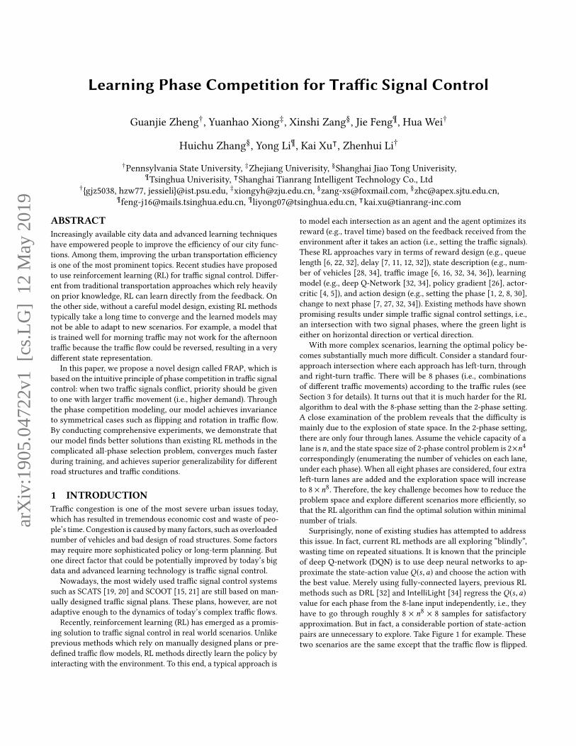
pairs are unnecessary to explore. Take Figure 1 for example. These
two scenarios are the same except that the traffic flow is flipped.
arX
iv:1
905.
0472
2v1
[cs
.LG
] 1
2 M
ay 2
019
(a) morning traffic
state definition:#cars on entering approach[North, East, South, West]
state: [1,1,1,5]
North
South
West East
North
South
West East
(b) afternoon traffic
state: [1,5,1,1]
Figure 1: Traffic (a) and (b) are flipped cases of each other.
0-degree rotation 90-degree rotation 180-degree rotation 270-degree rotation
no flipping
west-east flipping
Figure 2: All the variations based on rotation and flippingof the left-most case. Ideally, a RL model should handle allthese cases equally well.
Since such a flipping will result in a totally different state represen-
tation for existing methods, a RL agent which has learned the first
case still cannot handle the second case. But based on the common
sense, these two cases are almost identical and one would hope that
the model learned from the first case can handle the second case
or other similar cases. Furthermore, as shown in Figure 2, given
any particular state, one can generate seven other cases through
rotation and flipping. An ideal RL model is thus expected to handle
all eight cases even only one case is seen during training.
Based on the above observation, we propose a novel RL model
design called FRAP (which is invariant to symmetric operations like
Flip and Rotation and considersAll Phase configurations). The keyidea is that, instead of considering individual traffic movements,
one should focus on the relative relation between different traffic
movements. This idea is based on the intuitive principle of compe-
tition in traffic signal control: (1) larger traffic movement indicates
higher demand for green signal; and (2) when two signals conflict,
we should give the priority to the one with higher demand.
Inspired by this principle, FRAP first predicts the demand for
each signal phase, and then models the competition between phases.
Through the pair-wise phase competition modeling, FRAP is able
to achieve invariance to symmetries in traffic signal control (e.g.,
flipping and rotation). By leveraging such invariance and enabling
knowledge sharing across the symmetric states, FRAP successfully
reduces the exploration space to 16 × n4 samples from 64 × n8 (seeSection 4 for detailed analysis). Compared to existing RL-based
methods, FRAP finds better policies and converges much faster
under complex traffic control scenarios.
In summary, the main contributions of this paper include:
• We propose a novel model design FRAP for RL-based traffic signal
control. By capturing the competition relation between differ-
ent traffic movements, FRAP achieves invariance to symmetry
properties, which in turn leads to better solutions for the difficult
all-phase traffic signal control problem.
• We demonstrate that FRAP converges much faster than existing
RL methods during the learning process through comprehensive
experiments on real world data.
• We further demonstrate the superior generalizability of FRAP.Specifically, we show that FRAP can handle different road struc-
tures, different traffic flows, complex real-world phase settings,
as well as a multi-intersection environment.
2 RELATEDWORK
Traditional traffic signal control. Traffic signal control is a core
research topic in transportation field and existing methods can be
generally categorized into four classes.
Fixed-timed control [29] decides a traffic signal plan according
to human prior knowledge and the signal timing does not change
according to the real-time data.
Actuated methods [13, 24] define a set of rules and the traffic
signal is triggered according to the pre-defined rules and real-time
data. An example rule can be, to set the green signal for that traffic
movement if the queue length is longer than certain threshold.
Selection-based adaptive control methods first decide a set of traffic
signal plans and choose one that is the best for the current traffic
situation (based on traffic volume data received from loop sensors).
This method is widely deployed in today’s traffic signal control.
Commonly used systems include SCATS [19, 20], RHODES [25]
and SCOOT [15].
All the methods mentioned above highly rely on human knowl-
edge, as they require manually designed traffic signal plans or rules.
Optimization-based adaptive control approaches rely less on hu-
man knowledge and decide the traffic signal plans according to the
observed data. These approaches typically formulate traffic signal
control as an optimization problem under certain traffic flow model.
To make the optimization problems tractable, strong assumptions
about the model are often made. For example, a classical approach
is to optimize travel time by assuming uniform arrival rate [29, 33].
The traffic signal plan including cycle length and phase ratio can
then be calculated using a formula based on the traffic data. How-
ever, the model assumptions (e.g., uniform arrival rate [29, 33]) are
often too restricted and do not apply in the real world.
Learning for traffic signal control. Different from traditional
methods, learning-based traffic signal control does not require any
pre-defined traffic signal plan or traffic flow models. In particular,
reinforcement learning methods directly learns from intersections
with the world. In these methods, each intersection is an agent,
state is the quantitative description of the traffic condition at that
intersection, action is the traffic signal, and reward is a measure on
the transportation efficiency.
Existing RL methods differ in terms of state description of the en-
vironment (e.g., image of vehicle positions [6, 16, 32, 34, 36], queue
length [1–3, 34, 36], waiting time [7, 27, 34, 35]), action definition
(e.g., change to next phase [7, 27, 32, 34], setting a phase [1, 2, 8, 30]),
and reward design (e.g., queue length [6, 22, 32], delay [7, 11, 12, 32]).
1 2 3 4
5 6 7 8
00100001
The phase corresponding to the traffic signal in Figure (a) is phase C defined in Figure (d)
5
1
F
4
8
2
C
3
2 6
6 D
4
H
73
7
1
5 8
E
BA
G
White cell: non-conflicting phaseGrey cell: conflicting phase
Letters ‘A’ to ‘H’: eight phases for consideration
Conflict Matrix for Movement Signal
Movement SignalNorth
South
West East
North entering
approach Through movement on East entering approach
Left-turn movement on East entering approach
FE
H
G
H
C
D
G
A
BA D
F
C
E
B
Competing Matrix for Phase
Dark grey cell: competingLight grey cell: partial competing
White cell: no competing (with itself)
61
3 8 52
4 7
(a)
(b)
(d) (e)
(c)
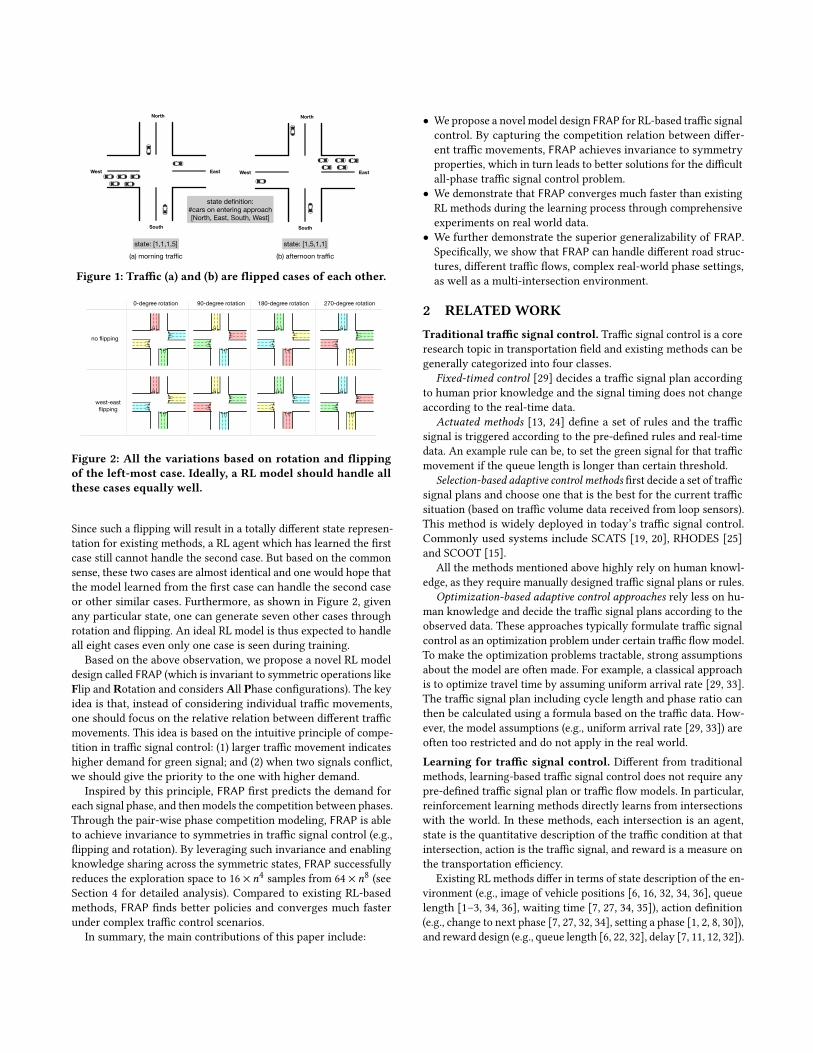
Figure 3: Illustration of preliminary definition.
In terms of algorithms, studies have utilized tabular methods (e.g.,
Q-learning [3, 11]) for discrete state space and approximation meth-
ods [17, 34], which can be further categorized into value based
(e.g., deep Q-Network [17, 32, 34]), policy based (e.g., policy gradi-
ent [26]), and actor critic [4, 5, 9].
However, to the best of our knowledge, none of these methods
have shown satisfactory results in complete 8-phase scenario for
one single intersection due to the large exploration space. In this
paper, we follow the universal principles of competition and invari-
ance in traffic signal control to design a novel model for efficient
exploration. Further, we adopt the distributed framework of Ape-X
DQN [14] as our base framework, which is shown to achieve the
state-of-the-art performance in playing Atari games. But our model
design can be adapted to other algorithmic frameworks including
policy based and actor critic based RL methods.
3 PROBLEM DEFINITION3.1 PreliminaryIn this paper, we investigate the traffic signal control in the sce-
nario of a single intersection. To illustrate the definitions, we use
the 4-approach intersection shown in Figure 3 as an example. But
the concepts can be easily generalized to different intersection
structures (e.g., different number of entering approaches).
• Entering approach: Each intersection has four entering ap-
proaches, named as North / South /West / East entering approach
(‘N’, ‘S’, ‘W’, ‘E’ for short) respectively. In Figure 3(a), we point
out the North entering approach.
• Traffic movement: A traffic movement is defined as the traffic
moving towards certain direction, i.e., left turn, through, and right
turn. In Figure 3(a), we show that there are 8 traffic movements.
Follow the traffic rules in most countries, right turn traffic can
pass regardless of the signal, but it needs to yield on a red light.
In addition, a traffic movement could occupy more than one lane
but this does not affect our model design because a traffic signal
controls a traffic movement instead of a lane.
• Movement signal: For each traffic movement, we can use one
bit with 1 as ‘green’ signal and 0 as ‘red’.
• Phase: We use an 8-bit vector p to represent a combination of
movement signals (i.e., a phase), as shown in Figure 3(b). As
indicated by the conflict matrix in Figure 3(d), some signals can-
not turn ‘green’ at the same time (e.g., signals #1 and #2). All
the non-conflicting signals will generate 8 valid paired-signal
phases (letters ‘A’ to ’H’ in Figure 3(c)) and 8 single-signal phases
(the diagonal cells in conflict matrix). Here we do not consider
the single-signal phase because in an isolated intersection, it is
always more efficient to use paried-signal phases.1
3.2 RL EnvironmentDriven by the idea of learning from the feedback, in this paper we
propose a reinforcement learning approach to traffic signal control.
In our problem, an agent can observe the traffic situation at an
isolated intersection (Figure 3(a)) and change the traffic signals
accordingly. The goal of the agent is to learn a policy for oper-
ating the signals which optimizes travel time. This traffic signal
control problem can be formulated as a Markov Decision Process
< S,A,P,R,γ > [31]:
Problem 1. Given the state observations set S, action set A, thereward function R is a function of S × A → R, specifically, Ra
s =
E[Rt+1 |St = s,At = a]. The agent aims to learn a policy π (At =a |St = s), which determines the best action a to take given state s , sothat the following expected discounted return is maximized:2
Gt = Rt+1 + γRt+2 + γ2Rt+3 + ... =
∞∑m=0
γmRt+m+1. (1)
For traffic signal control, our RL agent is defined as follows:
1When considering multiple intersections, single-signal phase might be necessary
because of the potential spill back.
2State transition probability matrix P is not described here because it is not explicitly
modeled in model-free methods.
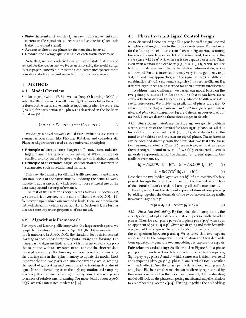
• State: the number of vehicles fvi on each traffic movement i andcurrent traffic signal phase (represented as one bit fsi for each
traffic movement signal).
• Action: to choose the phase for the next time interval.
• Reward: the average queue length of each traffic movement.
Note that, we use a relatively simple set of state features and
reward, for the reason that we focus on innovating the model design
in this paper. However, our method can easily incorporate more
complex state features and rewards for performance boosts.
4 METHOD4.1 Model OverviewSimilar to prior work [17, 34], we use Deep Q-learning (DQN) to
solve the RL problem. Basically, our DQN network takes the state
features on the traffic movements as input and predict the score (i.e.,
Q value) for each action (i.e., phase) as described in the Bellman
Equation [31]:
Q(st ,at ) = R(st ,at ) + γ maxQ(st+1,at+1). (2)
We design a novel network called FRAP (which is invariant to
symmetric operations like Flip and Rotation and considers AllPhase configurations) based on two universal principles:
• Principle of competition: Larger traffic movement indicates
higher demand for ‘green’ movement signal. When two signals
conflict, priority should be given to the one with higher demand.
• Principle of invariance: Signal control should be invariant to
symmetries such as rotation and flipping.
This way, the learning for different traffic movements and phases
can now occur at the same time by updating the same network
module (i.e., parameters), which leads to more efficient use of the
data samples and better performance.
The rest of this section is organized as follows. In Section 4.2,
we give a brief overview of the state-of-the-art Ape-X DQN [14]
framework, upon which our method is built. Then, we describe our
network design in details in Section 4.3. In Section 4.4, we further
discuss some important properties of our model.
4.2 Algorithmic FrameworkFor improved learning efficiency with the large search space, we
adopt the distributed framework Ape-X DQN [14] as our algorith-
mic framework. In Ape-X DQN, the standard deep reinforcement
learning is decomposed into two parts: acting and learning. Theacting part assigns multiple actors with different exploration poli-
cies to interact with an environment and to store the observed date
in a replay memory. The learning part is responsible for sampling
the training data in the replay memory to update the model. Most
importantly, the two parts can run concurrently while keeping
the speed of generating and consuming the training data almost
equal. In short, benefiting from the high exploration and sampling
efficiency, this framework can significantly boost the learning per-
formance of reinforcement learning. For more details about Ape-X
DQN, we refer interested readers to [14].
4.3 Phase Invariant Signal Control DesignAs we discussed before, training a RL agent for traffic signal control
is highly challenging due to the large search space. For instance,
for the four-approach intersection shown in Figure 3(a), assuming
there is only one lane on each traffic movement, the size of the
state space will be n8 × 8, where n is the capacity of a lane. Thus,
even with a small lane capacity (e.g., n = 10), DQN will require
billions of data samples to learn the relation between state, action
and reward. Further, intersections may vary in the geometry (e.g.,
3, 4, or 5 entering approaches) and the signal setting (i.e., different
combination of traffic movement signals). It is very inefficient if a
different agent needs to be learned for each different intersection.
To address these challenges, we design our model based on the
two principles outlined in Section 4.1, so that it can learn more
efficiently from data and also be easily adapted to different inter-
section structures. We divide the prediction of phase score (i.e., Q
value) into three stages: phase demand modeling, phase pair embed-ding, and phase pair competition. Figure 4 shows an overview of our
method. Next we describe these three stages in details.
4.3.1 Phase Demand Modeling. In this stage, our goal is to obtain
a representation of the demand for each signal phase. Recall that
for any traffic movement i, i ∈ {1, . . . , 8}, its state includes the
number of vehicles and the current signal phase. These features
can be obtained directly from the simulator. We first take these
two features, denoted as fvi and fsi respectively, as input, and pass
them through a neural network of two fully-connected layers to
generate a representation of the demand for ‘green’ signal on this
traffic movement, di .
hvi = ReLU (Wv fvi + bv ), hsi = ReLU (Ws fsi + b
s ). (3)
di = ReLU (Wh [hvi , hsi ] + b
h ). (4)
Note that the two hidden layer vectors hvi , hsi are combined before
passed through the output layer. Further, the learned parameters
of the neural network are shared among all traffic movements.
Finally, we obtain the demand representation of any phase pby adding together the demands of the two non-conflicting traffic
movement signals in p:
d(p) = di + dj , where pi = pj = 1. (5)
4.3.2 Phase Pair Embedding. By the principle of competition, the
score (priority) of a phase depends on its competition with the other
phases. Thus, for each phase p, we form phase pairs (p, q)where q isan opponent of p (i.e., q , p). Given a pair (p, q) and their demands,
our goal of this stage is therefore to obtain a representation of
the competition between p and q. We observe that two aspects
are essential to the competition: their relation and their demands.
Consequently, we generate two embeddings to capture the aspects.
Pair relation embedding: As illustrated in Figure 3(e), a phase
pair p and q can have two different relations: partial competing
(light grey, e.g., phase A and B, which shares one traffic movement)
and competing (dark grey, e.g., phase A and D, which totally conflict
with each other). Once the phase pair is determined, (e.g., phase A
and phase B), their conflict matrix can be directly represented by
the corresponding cell in the matrix in Figure 3(d). Our embedding
model will look up the phase competingmatrix andmap the relation
to an embedding vector e(p, q). Putting together the embedding
1
4
5
8
Phase demand modeling Phase pair competition
Phase H
7 phase pairs
8 phases
2 com
peting
phase
s
FE
HG
H
CD
GA
BA D
F
C
E
B
Pair relation embedding
Phase pair embedding
Table look up
Phase A
Pair demand embedding
Phase score
Phase pair relation representation
Phase pair demand representation
Phase competition representation
Traffic movement demand
Pairwise competition result
1x1 conv
1x1 conv
1x1 conv
Element-wise multiplication
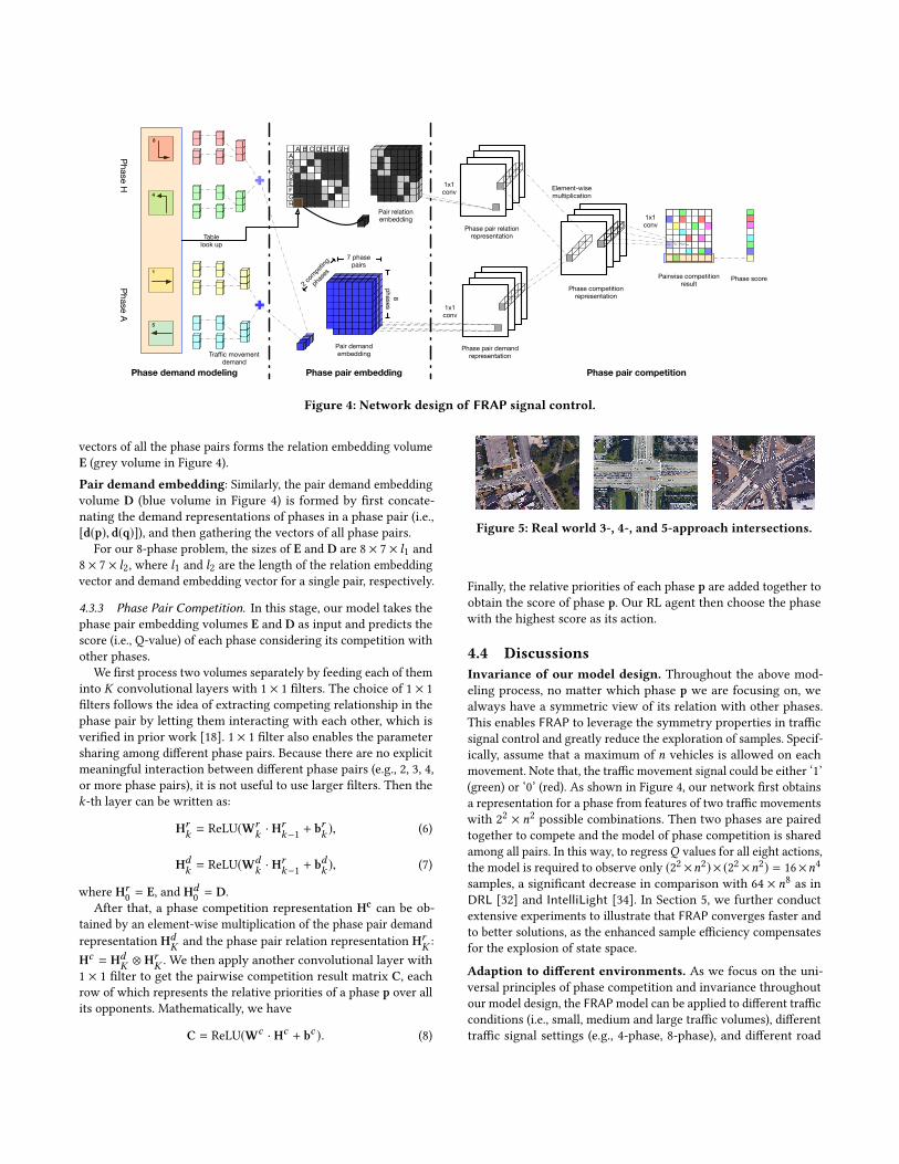
Figure 4: Network design of FRAP signal control.
vectors of all the phase pairs forms the relation embedding volume
E (grey volume in Figure 4).
Pair demand embedding: Similarly, the pair demand embedding
volume D (blue volume in Figure 4) is formed by first concate-
nating the demand representations of phases in a phase pair (i.e.,
[d(p), d(q)]), and then gathering the vectors of all phase pairs.
For our 8-phase problem, the sizes of E and D are 8 × 7 × l1 and8 × 7 × l2, where l1 and l2 are the length of the relation embedding
vector and demand embedding vector for a single pair, respectively.
4.3.3 Phase Pair Competition. In this stage, our model takes the
phase pair embedding volumes E and D as input and predicts the
score (i.e., Q-value) of each phase considering its competition with
other phases.
We first process two volumes separately by feeding each of them
into K convolutional layers with 1 × 1 filters. The choice of 1 × 1
filters follows the idea of extracting competing relationship in the
phase pair by letting them interacting with each other, which is
verified in prior work [18]. 1 × 1 filter also enables the parameter
sharing among different phase pairs. Because there are no explicit
meaningful interaction between different phase pairs (e.g., 2, 3, 4,
or more phase pairs), it is not useful to use larger filters. Then the
k-th layer can be written as:
Hrk = ReLU(Wr
k · Hrk−1 + b
rk ), (6)
Hdk = ReLU(Wd
k · Hrk−1 + b
dk ), (7)
where Hr0= E, and Hd
0= D.
After that, a phase competition representation Hccan be ob-
tained by an element-wise multiplication of the phase pair demand
representation HdK and the phase pair relation representation Hr
K :
Hc = HdK ⊗ Hr
K . We then apply another convolutional layer with
1 × 1 filter to get the pairwise competition result matrix C, eachrow of which represents the relative priorities of a phase p over all
its opponents. Mathematically, we have
C = ReLU(Wc · Hc + bc ). (8)
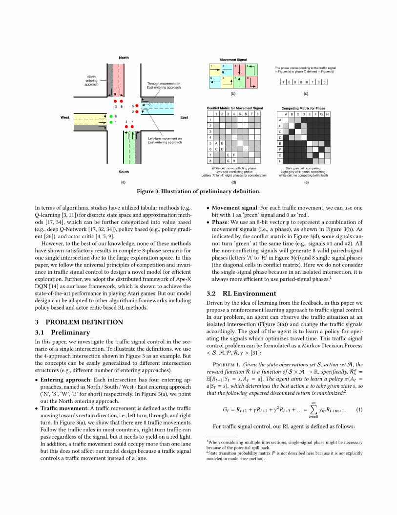
Figure 5: Real world 3-, 4-, and 5-approach intersections.
Finally, the relative priorities of each phase p are added together to
obtain the score of phase p. Our RL agent then choose the phase
with the highest score as its action.
4.4 DiscussionsInvariance of our model design. Throughout the above mod-
eling process, no matter which phase p we are focusing on, we
always have a symmetric view of its relation with other phases.
This enables FRAP to leverage the symmetry properties in traffic
signal control and greatly reduce the exploration of samples. Specif-
ically, assume that a maximum of n vehicles is allowed on each
movement. Note that, the traffic movement signal could be either ‘1’
(green) or ‘0’ (red). As shown in Figure 4, our network first obtains
a representation for a phase from features of two traffic movements
with 22 × n2 possible combinations. Then two phases are paired
together to compete and the model of phase competition is shared
among all pairs. In this way, to regressQ values for all eight actions,
the model is required to observe only (22 ×n2) × (22 ×n2) = 16×n4samples, a significant decrease in comparison with 64 × n8 as inDRL [32] and IntelliLight [34]. In Section 5, we further conduct
extensive experiments to illustrate that FRAP converges faster and
to better solutions, as the enhanced sample efficiency compensates
for the explosion of state space.
Adaption to different environments. As we focus on the uni-
versal principles of phase competition and invariance throughout
our model design, the FRAPmodel can be applied to different traffic
conditions (i.e., small, medium and large traffic volumes), different
traffic signal settings (e.g., 4-phase, 8-phase), and different road
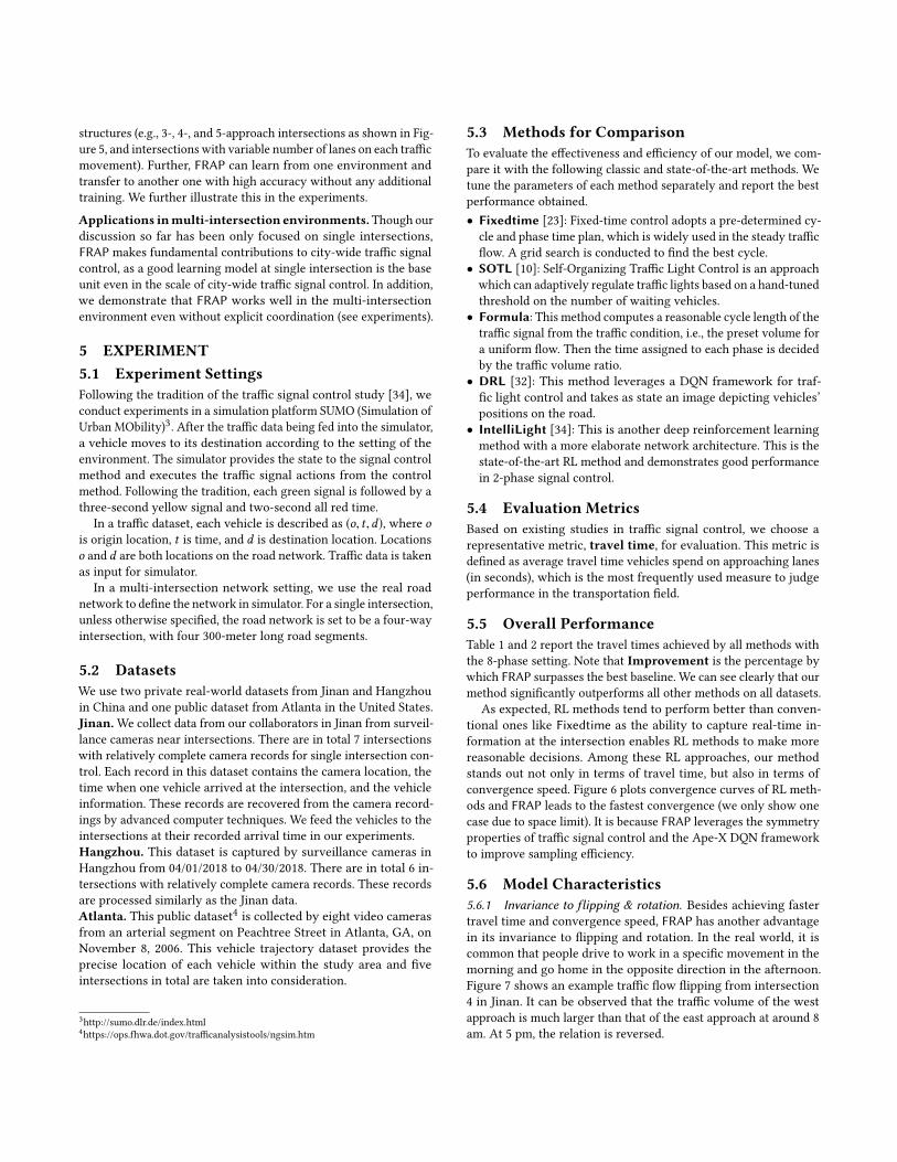
structures (e.g., 3-, 4-, and 5-approach intersections as shown in Fig-
ure 5, and intersections with variable number of lanes on each traffic
movement). Further, FRAP can learn from one environment and
transfer to another one with high accuracy without any additional
training. We further illustrate this in the experiments.
Applications inmulti-intersection environments.Though ourdiscussion so far has been only focused on single intersections,
FRAP makes fundamental contributions to city-wide traffic signal
control, as a good learning model at single intersection is the base
unit even in the scale of city-wide traffic signal control. In addition,
we demonstrate that FRAP works well in the multi-intersection
environment even without explicit coordination (see experiments).
5 EXPERIMENT5.1 Experiment SettingsFollowing the tradition of the traffic signal control study [34], we
conduct experiments in a simulation platform SUMO (Simulation of
Urban MObility)3. After the traffic data being fed into the simulator,
a vehicle moves to its destination according to the setting of the
environment. The simulator provides the state to the signal control
method and executes the traffic signal actions from the control
method. Following the tradition, each green signal is followed by a
three-second yellow signal and two-second all red time.
In a traffic dataset, each vehicle is described as (o, t ,d), where ois origin location, t is time, and d is destination location. Locations
o and d are both locations on the road network. Traffic data is taken
as input for simulator.
In a multi-intersection network setting, we use the real road
network to define the network in simulator. For a single intersection,
unless otherwise specified, the road network is set to be a four-way
intersection, with four 300-meter long road segments.
5.2 DatasetsWe use two private real-world datasets from Jinan and Hangzhou
in China and one public dataset from Atlanta in the United States.
Jinan.We collect data from our collaborators in Jinan from surveil-
lance cameras near intersections. There are in total 7 intersections
with relatively complete camera records for single intersection con-
trol. Each record in this dataset contains the camera location, the
time when one vehicle arrived at the intersection, and the vehicle
information. These records are recovered from the camera record-
ings by advanced computer techniques. We feed the vehicles to the
intersections at their recorded arrival time in our experiments.
Hangzhou. This dataset is captured by surveillance cameras in
Hangzhou from 04/01/2018 to 04/30/2018. There are in total 6 in-
tersections with relatively complete camera records. These records
are processed similarly as the Jinan data.
Atlanta. This public dataset4 is collected by eight video cameras
from an arterial segment on Peachtree Street in Atlanta, GA, on
November 8, 2006. This vehicle trajectory dataset provides the
precise location of each vehicle within the study area and five
intersections in total are taken into consideration.
3http://sumo.dlr.de/index.html
4https://ops.fhwa.dot.gov/trafficanalysistools/ngsim.htm
5.3 Methods for ComparisonTo evaluate the effectiveness and efficiency of our model, we com-
pare it with the following classic and state-of-the-art methods. We
tune the parameters of each method separately and report the best
performance obtained.
• Fixedtime [23]: Fixed-time control adopts a pre-determined cy-
cle and phase time plan, which is widely used in the steady traffic
flow. A grid search is conducted to find the best cycle.
• SOTL [10]: Self-Organizing Traffic Light Control is an approach
which can adaptively regulate traffic lights based on a hand-tuned
threshold on the number of waiting vehicles.
• Formula: This method computes a reasonable cycle length of the
traffic signal from the traffic condition, i.e., the preset volume for
a uniform flow. Then the time assigned to each phase is decided
by the traffic volume ratio.
• DRL [32]: This method leverages a DQN framework for traf-
fic light control and takes as state an image depicting vehicles’
positions on the road.
• IntelliLight [34]: This is another deep reinforcement learning
method with a more elaborate network architecture. This is the
state-of-the-art RL method and demonstrates good performance
in 2-phase signal control.
5.4 Evaluation MetricsBased on existing studies in traffic signal control, we choose a
representative metric, travel time, for evaluation. This metric is
defined as average travel time vehicles spend on approaching lanes
(in seconds), which is the most frequently used measure to judge
performance in the transportation field.
5.5 Overall PerformanceTable 1 and 2 report the travel times achieved by all methods with
the 8-phase setting. Note that Improvement is the percentage bywhich FRAP surpasses the best baseline. We can see clearly that our
method significantly outperforms all other methods on all datasets.
As expected, RL methods tend to perform better than conven-
tional ones like Fixedtime as the ability to capture real-time in-
formation at the intersection enables RL methods to make more
reasonable decisions. Among these RL approaches, our method
stands out not only in terms of travel time, but also in terms of
convergence speed. Figure 6 plots convergence curves of RL meth-
ods and FRAP leads to the fastest convergence (we only show one
case due to space limit). It is because FRAP leverages the symmetry
properties of traffic signal control and the Ape-X DQN framework
to improve sampling efficiency.
5.6 Model Characteristics5.6.1 Invariance to flipping & rotation. Besides achieving faster
travel time and convergence speed, FRAP has another advantage
in its invariance to flipping and rotation. In the real world, it is
common that people drive to work in a specific movement in the
morning and go home in the opposite direction in the afternoon.
Figure 7 shows an example traffic flow flipping from intersection
4 in Jinan. It can be observed that the traffic volume of the west
approach is much larger than that of the east approach at around 8
am. At 5 pm, the relation is reversed.
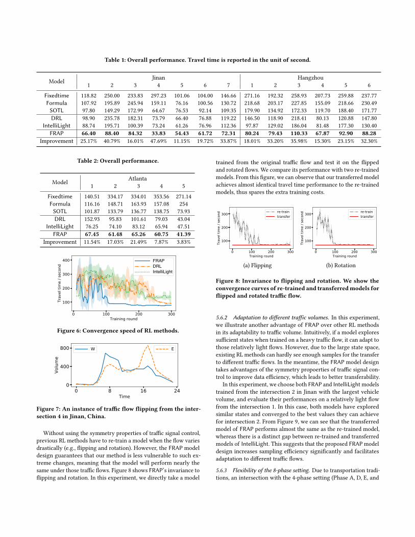
Table 1: Overall performance. Travel time is reported in the unit of second.
Model
Jinan Hangzhou
1 2 3 4 5 6 7 1 2 3 4 5 6
Fixedtime 118.82 250.00 233.83 297.23 101.06 104.00 146.66 271.16 192.32 258.93 207.73 259.88 237.77
Formula 107.92 195.89 245.94 159.11 76.16 100.56 130.72 218.68 203.17 227.85 155.09 218.66 230.49
SOTL 97.80 149.29 172.99 64.67 76.53 92.14 109.35 179.90 134.92 172.33 119.70 188.40 171.77
DRL 98.90 235.78 182.31 73.79 66.40 76.88 119.22 146.50 118.90 218.41 80.13 120.88 147.80
IntelliLight 88.74 195.71 100.39 73.24 61.26 76.96 112.36 97.87 129.02 186.04 81.48 177.30 130.40
FRAP 66.40 88.40 84.32 33.83 54.43 61.72 72.31 80.24 79.43 110.33 67.87 92.90 88.28Improvement 25.17% 40.79% 16.01% 47.69% 11.15% 19.72% 33.87% 18.01% 33.20% 35.98% 15.30% 23.15% 32.30%
Table 2: Overall performance.
Model
Atlanta
1 2 3 4 5
Fixedtime 140.51 334.17 334.01 353.56 271.14
Formula 116.16 148.71 163.93 157.08 254
SOTL 101.87 133.79 136.77 138.75 73.93
DRL 152.93 95.83 101.61 79.03 43.04
IntelliLight 76.25 74.10 83.12 65.94 47.51
FRAP 67.45 61.48 65.26 60.75 41.39Improvement 11.54% 17.03% 21.49% 7.87% 3.83%
0 100 200 300Training round
100
200
300
400
Trav
el ti
me
/ sec
ond
FRAPDRL IntelliLight
Figure 6: Convergence speed of RL methods.
0 8 16 24Time
0
400
800
Volu
me
W E
Figure 7: An instance of traffic flow flipping from the inter-section 4 in Jinan, China.
Without using the symmetry properties of traffic signal control,
previous RL methods have to re-train a model when the flow varies
drastically (e.g., flipping and rotation). However, the FRAP model
design guarantees that our method is less vulnerable to such ex-
treme changes, meaning that the model will perform nearly the
same under those traffic flows. Figure 8 shows FRAP’s invariance toflipping and rotation. In this experiment, we directly take a model
trained from the original traffic flow and test it on the flipped
and rotated flows. We compare its performance with two re-trained
models. From this figure, we can observe that our transferred model
achieves almost identical travel time performance to the re-trained
models, thus spares the extra training costs.
0 100 200 300Training round
100
200
300Tr
avel
tim
e / s
econ
d re-traintransfer
0 100 200 300Training round
100
200
300
Trav
el ti
me
/ sec
ond re-train
transfer
(a) Flipping (b) Rotation
Figure 8: Invariance to flipping and rotation. We show theconvergence curves of re-trained and transferredmodels forflipped and rotated traffic flow.
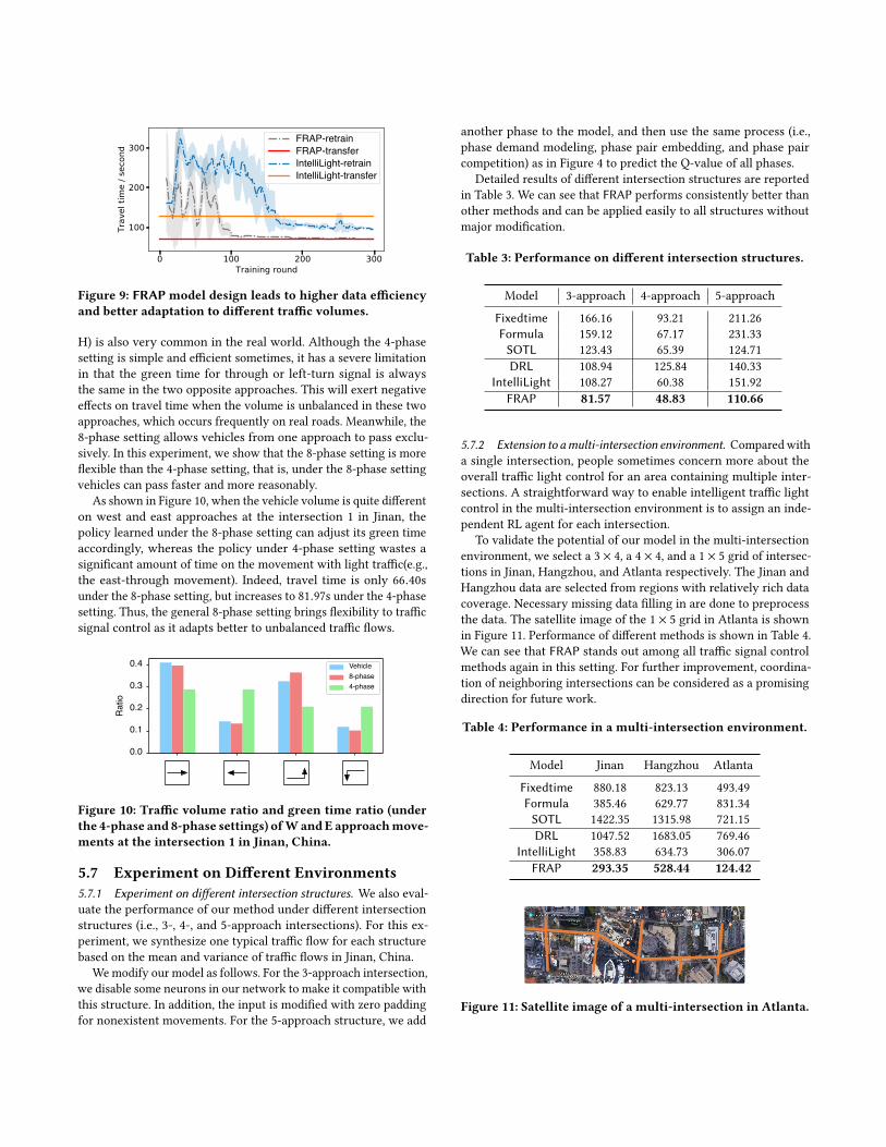
5.6.2 Adaptation to different traffic volumes. In this experiment,
we illustrate another advantage of FRAP over other RL methods
in its adaptability to traffic volume. Intuitively, if a model explores
sufficient states when trained on a heavy traffic flow, it can adapt to
those relatively light flows. However, due to the large state space,
existing RL methods can hardly see enough samples for the transfer
to different traffic flows. In the meantime, the FRAP model design
takes advantages of the symmetry propoerties of traffic signal con-
trol to improve data efficiency, which leads to better transferability.
In this experiment, we choose both FRAP and IntelliLightmodels
trained from the intersection 2 in Jinan with the largest vehicle
volume, and evaluate their performances on a relatively light flow
from the intersection 1. In this case, both models have explored
similar states and converged to the best values they can achieve
for intersection 2. From Figure 9, we can see that the transferred
model of FRAP performs almost the same as the re-trained model,
whereas there is a distinct gap between re-trained and transferred
models of IntelliLight. This suggests that the proposed FRAPmodel
design increases sampling efficiency significantly and facilitates
adaptation to different traffic flows.
5.6.3 Flexibility of the 8-phase setting. Due to transportation tradi-
tions, an intersection with the 4-phase setting (Phase A, D, E, and
0 100 200 300Training round
100
200
300
Trav
el ti
me
/ sec
ond
FRAP-retrainFRAP-transferIntelliLight-retrainIntelliLight-transfer
Figure 9: FRAP model design leads to higher data efficiencyand better adaptation to different traffic volumes.
H) is also very common in the real world. Although the 4-phase
setting is simple and efficient sometimes, it has a severe limitation
in that the green time for through or left-turn signal is always
the same in the two opposite approaches. This will exert negative
effects on travel time when the volume is unbalanced in these two
approaches, which occurs frequently on real roads. Meanwhile, the
8-phase setting allows vehicles from one approach to pass exclu-
sively. In this experiment, we show that the 8-phase setting is more
flexible than the 4-phase setting, that is, under the 8-phase setting
vehicles can pass faster and more reasonably.
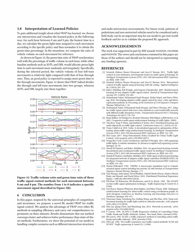
As shown in Figure 10, when the vehicle volume is quite different
on west and east approaches at the intersection 1 in Jinan, the
policy learned under the 8-phase setting can adjust its green time
accordingly, whereas the policy under 4-phase setting wastes a
significant amount of time on the movement with light traffic(e.g.,
the east-through movement). Indeed, travel time is only 66.40s
under the 8-phase setting, but increases to 81.97s under the 4-phase
setting. Thus, the general 8-phase setting brings flexibility to traffic
signal control as it adapts better to unbalanced traffic flows.
0.0
0.1
0.2
0.3
0.4
Ratio
Vehicle8-phase4-phase
Figure 10: Traffic volume ratio and green time ratio (underthe 4-phase and 8-phase settings) ofWandE approachmove-ments at the intersection 1 in Jinan, China.
5.7 Experiment on Different Environments5.7.1 Experiment on different intersection structures. We also eval-
uate the performance of our method under different intersection
structures (i.e., 3-, 4-, and 5-approach intersections). For this ex-
periment, we synthesize one typical traffic flow for each structure
based on the mean and variance of traffic flows in Jinan, China.
We modify our model as follows. For the 3-approach intersection,
we disable some neurons in our network to make it compatible with
this structure. In addition, the input is modified with zero padding
for nonexistent movements. For the 5-approach structure, we add
another phase to the model, and then use the same process (i.e.,
phase demand modeling, phase pair embedding, and phase pair
competition) as in Figure 4 to predict the Q-value of all phases.
Detailed results of different intersection structures are reported
in Table 3. We can see that FRAP performs consistently better than
other methods and can be applied easily to all structures without
major modification.
Table 3: Performance on different intersection structures.
Model 3-approach 4-approach 5-approach
Fixedtime 166.16 93.21 211.26
Formula 159.12 67.17 231.33
SOTL 123.43 65.39 124.71
DRL 108.94 125.84 140.33
IntelliLight 108.27 60.38 151.92
FRAP 81.57 48.83 110.66
5.7.2 Extension to amulti-intersection environment. Comparedwith
a single intersection, people sometimes concern more about the
overall traffic light control for an area containing multiple inter-
sections. A straightforward way to enable intelligent traffic light
control in the multi-intersection environment is to assign an inde-
pendent RL agent for each intersection.
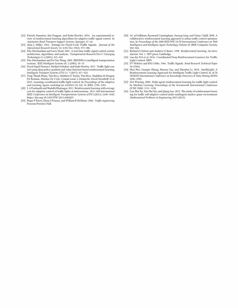
To validate the potential of our model in the multi-intersection
environment, we select a 3 × 4, a 4 × 4, and a 1 × 5 grid of intersec-
tions in Jinan, Hangzhou, and Atlanta respectively. The Jinan and
Hangzhou data are selected from regions with relatively rich data
coverage. Necessary missing data filling in are done to preprocess
the data. The satellite image of the 1 × 5 grid in Atlanta is shown
in Figure 11. Performance of different methods is shown in Table 4.
We can see that FRAP stands out among all traffic signal control
methods again in this setting. For further improvement, coordina-
tion of neighboring intersections can be considered as a promising
direction for future work.
Table 4: Performance in a multi-intersection environment.
Model Jinan Hangzhou Atlanta
Fixedtime 880.18 823.13 493.49
Formula 385.46 629.77 831.34
SOTL 1422.35 1315.98 721.15
DRL 1047.52 1683.05 769.46
IntelliLight 358.83 634.73 306.07
FRAP 293.35 528.44 124.42
Figure 11: Satellite image of a multi-intersection in Atlanta.
5.8 Interpretation of Learned PoliciesTo gain additional insight about what FRAP has learned, we choose
one intersection and visualize the learned policy in the following
way: for each hour between 8 am and 8 pm, the busiest time in a
day, we calculate the green light time assigned to each movement
according to the specific policy and then normalize it to obtain the
green time percentage. In the meantime, we compute the ratio of
vehicle volume on each movement for reference.
As shown in Figure 12, the green time ratio of FRAP synchronizeswell with the percentage of traffic volume in each hour, while other
baseline methods such as SOTL and DRL would allocate green light
time to each movement more randomly and irregularly. Specifically,
during the selected period, the vehicle volume of four left-turn
movements is relatively light compared with that of four through
ones. Thus, an good policy is expected to assign more green time to
the through movements. Figure 12 shows that FRAP indeed divides
the through and left-turn movements into two groups, whereas
SOTL and DRL largely mix them together.
0.00
0.15
0.30Vehicle Ratio
0.00
0.15
0.30
0.00
0.15
0.30SOTL
9 12 15 180.00
0.15
0.30DRL
Time
Ratio
12
34
56
78
FRAP
Figure 12: Traffic volume ratio and green time ratio of threetraffic signal control methods for each movement between8 am and 8 pm. The number from 1 to 8 indicates a specificmovement signal described in Figure 3(b).
6 CONCLUSIONIn this paper, inspired by the universal principles of competition
and invariance, we propose a novel RL model FRAP for traffic
signal control. We analyze the advantage of FRAP over other RL
methods in sampling efficiency and carry out comprehensive ex-
periments on three datasets. Results demonstrate that our method
converges faster and achieves better performance than state-of-the-
art methods. Furthermore, we show the potential of our model in
handling complex scenarios such as different intersection structures
and multi-intersection environments. For future work, patterns of
pedestrians and non-motorized vehicles need to be considered and a
field study can be an important step for our model to get real-world
feedback and for us to validate the proposed RL approach.
ACKNOWLEDGEMENTSThe work was supported in part by NSF awards #1652525, #1618448,
and #1639150. The views and conclusions contained in this paper are
those of the authors and should not be interpreted as representing
any funding agencies.
REFERENCES[1] Monireh Abdoos, Nasser Mozayani, and Ana LC Bazzan. 2011. Traffic light
control in non-stationary environments based on multi agent Q-learning. In
Intelligent Transportation Systems (ITSC), 2011 14th International IEEE Conferenceon. IEEE, 1580–1585.
[2] Monireh Abdoos, Nasser Mozayani, and Ana LC Bazzan. 2014. Hierarchical
control of traffic signals using Q-learning with tile coding. Applied intelligence40, 2 (2014), 201–213.
[3] Baher Abdulhai, Rob Pringle, and Grigoris J Karakoulas. 2003. Reinforcement
learning for true adaptive traffic signal control. Journal of Transportation Engi-neering 129, 3 (2003), 278–285.
[4] Mohammad Aslani, Mohammad Saadi Mesgari, Stefan Seipel, and Marco Wier-
ing. 2018. Developing adaptive traffic signal control by actor–critic and direct
exploration methods. In Proceedings of the Institution of Civil Engineers-Transport.Thomas Telford Ltd, 1–10.
[5] Mohammad Aslani, Mohammad Saadi Mesgari, and Marco Wiering. 2017. Adap-
tive traffic signal control with actor-critic methods in a real-world traffic network
with different traffic disruption events. Transportation Research Part C: EmergingTechnologies 85 (2017), 732–752.
[6] Bram Bakker, M Steingrover, Roelant Schouten, EHJ Nijhuis, LJHM Kester, et al.
2005. Cooperative multi-agent reinforcement learning of traffic lights. (2005).
[7] Tim Brys, Tong T Pham, and Matthew E Taylor. 2014. Distributed learning and
multi-objectivity in traffic light control. Connection Science 26, 1 (2014), 65–83.[8] Vinny Cahill et al. 2010. Soilse: A decentralized approach to optimization of fluc-
tuating urban traffic using reinforcement learning. In Intelligent TransportationSystems (ITSC), 2010 13th International IEEE Conference on. IEEE, 531–538.
[9] Noe Casas. 2017. Deep Deterministic Policy Gradient for Urban Traffic Light
Control. arXiv preprint arXiv:1703.09035 (2017).[10] Seung-Bae Cools, Carlos Gershenson, and Bart D’Hooghe. 2013. Self-organizing
traffic lights: A realistic simulation. In Advances in applied self-organizing systems.Springer, 45–55.
[11] Samah El-Tantawy and Baher Abdulhai. 2010. An agent-based learning towards
decentralized and coordinated traffic signal control. In Intelligent TransportationSystems (ITSC), 2010 13th International IEEE Conference on. IEEE, 665–670.
[12] Samah El-Tantawy and Baher Abdulhai. 2012. Multi-agent reinforcement learning
for integrated network of adaptive traffic signal controllers (MARLIN-ATSC). In
Intelligent Transportation Systems (ITSC), 2012 15th International IEEE Conferenceon. IEEE, 319–326.
[13] Martin Fellendorf. 1994. VISSIM: A microscopic simulation tool to evaluate
actuated signal control including bus priority. In 64th Institute of TransportationEngineers Annual Meeting. Springer, 1–9.
[14] Dan Horgan, John Quan, David Budden, Gabriel Barth-Maron, Matteo Hessel,
Hado van Hasselt, and David Silver. 2018. Distributed Prioritized Experience
Replay. CoRR abs/1803.00933 (2018).
[15] PB Hunt, DI Robertson, RD Bretherton, and M Cr Royle. 1982. The SCOOT
on-line traffic signal optimisation technique. Traffic Engineering & Control 23, 4(1982).
[16] Lior Kuyer, Shimon Whiteson, Bram Bakker, and Nikos Vlassis. 2008. Multiagent
reinforcement learning for urban traffic control using coordination graphs. In
Joint European Conference on Machine Learning and Knowledge Discovery inDatabases. Springer, 656–671.
[17] Xiaoyuan Liang, Xunsheng Du, Guiling Wang, and Zhu Han. 2018. Deep rein-
forcement learning for traffic light control in vehicular networks. arXiv preprintarXiv:1803.11115 (2018).
[18] Min Lin, Qiang Chen, and Shuicheng Yan. 2013. Network in network. arXivpreprint arXiv:1312.4400 (2013).
[19] P Lowrie. 1990. SCATS–A Traffic Responsive Method of Controlling Urban
Traffic. Roads and Traffic Authority, Sydney. New South Wales, Australia (1990).[20] PR Lowrie. 1992. SCATS–a traffic responsive method of controlling urban traffic.
Roads and traffic authority. NSW, Australia (1992).[21] JYK Luk. 1984. Two traffic-responsive area traffic control methods: SCAT and
SCOOT. Traffic engineering & control 25, 1 (1984).
[22] Patrick Mannion, Jim Duggan, and Enda Howley. 2016. An experimental re-
view of reinforcement learning algorithms for adaptive traffic signal control. In
Autonomic Road Transport Support Systems. Springer, 47–66.[23] Alan J. Miller. 1963. Settings for Fixed-Cycle Traffic Signals. Journal of the
Operational Research Society 14, 4 (01 Dec 1963), 373–386.
[24] Pitu Mirchandani and Larry Head. 2001. A real-time traffic signal control system:
architecture, algorithms, and analysis. Transportation Research Part C: EmergingTechnologies 9, 6 (2001), 415–432.
[25] Pitu Mirchandani and Fei-Yue Wang. 2005. RHODES to intelligent transportation
systems. IEEE Intelligent Systems 20, 1 (2005), 10–15.[26] Seyed Sajad Mousavi, Michael Schukat, and Enda Howley. 2017. Traffic light con-
trol using deep policy-gradient and value-function-based reinforcement learning.
Intelligent Transport Systems (ITS) 11, 7 (2017), 417–423.[27] Tong Thanh Pham, Tim Brys, Matthew E Taylor, Tim Brys, Madalina M Drugan,
PA Bosman, Martine-De Cock, Cosmin Lazar, L Demarchi, David Steenhoff, et al.
2013. Learning coordinated traffic light control. In Proceedings of the Adaptiveand Learning Agents workshop (at AAMAS-13), Vol. 10. IEEE, 1196–1201.
[28] L A Prashanth and Shalabh Bhatnagar. 2011. Reinforcement learningwith average
cost for adaptive control of traffic lights at intersections. 2011 14th InternationalIEEE Conference on Intelligent Transportation Systems (ITSC) (2011), 1640–1645.https://doi.org/10.1109/ITSC.2011.6082823
[29] Roger P Roess, Elena S Prassas, and William R McShane. 2004. Traffic engineering.Pearson/Prentice Hall.
[30] As’ ad Salkham, Raymond Cunningham, Anurag Garg, and Vinny Cahill. 2008. A
collaborative reinforcement learning approach to urban traffic control optimiza-
tion. In Proceedings of the 2008 IEEE/WIC/ACM International Conference on WebIntelligence and Intelligent Agent Technology-Volume 02. IEEE Computer Society,
560–566.
[31] Richard S Sutton and Andrew G Barto. 1998. Reinforcement learning: An intro-duction. Vol. 1. MIT press Cambridge.
[32] van der Pol et al. 2016. Coordinated Deep Reinforcement Learners for Traffic
Light Control. NIPS.
[33] FV Webster and BM Cobbe. 1966. Traffic Signals. Road Research Technical Paper56 (1966).
[34] Hua Wei, Guanjie Zheng, Huaxiu Yao, and Zhenhui Li. 2018. IntelliLight: A
Reinforcement Learning Approach for Intelligent Traffic Light Control. In ACMSIGKDD International Conference on Knowledge Discovery & Data Mining (KDD).2496–2505.
[35] MA Wiering. 2000. Multi-agent reinforcement learning for traffic light control.
In Machine Learning: Proceedings of the Seventeenth International Conference(ICML’2000). 1151–1158.
[36] Lun-Hui Xu, Xin-Hai Xia, and Qiang Luo. 2013. The study of reinforcement learn-
ing for traffic self-adaptive control under multiagent markov game environment.
Mathematical Problems in Engineering 2013 (2013).