Learning Probabilistic Models: An Expected Utility Maximization

Journal of Machine Learning Research 4 (2003) 257-291 Submitted 4/03; Published 7/03

Learning Probabilistic Models: An Expected UtilityMaximization Approach

Craig Friedman CRAIG [email protected]

Sven Sandow SVEN [email protected]

Standard & Poor’sRisk Solutions Group55 Water StreetNew York, NY 10041

Editors: David Maxwell Chickering

AbstractWe consider the problem of learning a probabilistic model from the viewpoint of an expected util-ity maximizing decision maker/investor who would use the model to make decisions (bets), whichresult in well defined payoffs. In our new approach, we seek good out-of-sample model perfor-mance by considering a one-parameter family of Pareto optimal models, which we define in termsof consistency with the training data and consistency with a prior (benchmark) model. We measurethe former by means of the large-sample distribution of a vector of sample-averaged features, andthe latter by means of a generalized relative entropy. We express each Pareto optimal model asthe solution of a strictly convex optimization problem and its strictly concave (and tractable) dual.Each dual problem is a regularized maximization of expected utility over a well-defined family offunctions. Each Pareto optimal model is robust: maximizing worst-case outperformance relative tothe benchmark model. Finally, we select the Pareto optimal model with maximum (out-of-sample)expected utility. We show that our method reduces to the minimum relative entropy method if andonly if the utility function is a member of a three-parameter logarithmic family.Keywords: Learning Probabilistic Models, Expected Utility, Relative Entropy, Pareto Optimality,Robustness

1. Introduction

From the viewpoint of a rational decision maker in an uncertain world, the efficacy of a probabilisticmodel is directly related to the quality of the decisions that he makes, based on the model. If, forexample, the decision maker is an investor in a financial market, a probabilistic market model canbe used by the investor to design an optimal investment strategy; the efficacy of the model should bejudged by the success of this (optimal with respect to the model) strategy. Should the decision makerbuild a model, he ought to take this into account. In principle, standard approaches to probabilisticmodeling (see, for example, Vapnik, 1999, Berger, 1985, or Hastie, Tibshirani, and Friedman,2001) allow for the model builder to incorporate the decision consequences of a model, usually interms of a risk functional or a loss function. However, these approaches often give no guidance as tohow to construct, from first principles, a risk functional or a loss function. In this paper, we proposea new approach to model building that takesexplicitly into account the decision consequences ofthe model; we measure these decision consequences by the success of the strategy that a rationalinvestor (who believes the model) would choose to place bets in a horse race (see, for example,

c©2003 Craig Friedman and Sven Sandow.

FRIEDMAN AND SANDOW

Cover and Thomas, 1991 for a discussion of the horse race). In particular, we monetize the decisionconsequences by assuming that there is a market with payoffs associated with each state (the horserace). The assumption of a rational investor who bets on horses allows us to relate the modeluser’s decisions and their consequences to the model itself; as we shall see, this assumption leadsto tractable models. Our approach combines ideas from maximum entropy modeling and utilitytheory.

Maximum entropy inference, introduced by Jaynes (1957, 1982, 1984) in the context of sta-tistical physics, has been successfully applied to image processing (see, for example, Wu, 1997,or Gull and Daniell, 1978) as well as to a wide range of problems in biology (see, for example,Burnham and Anderson, 2002), finance (see, for example, Avellaneda, 1998, Avellaneda et al.,1997, Samperi, 1997, Gulko, 2002 and Frittelli, 2000) and economics (see, for example, Golanet al., 1996). The basic idea of the maximum entropy approach is that one chooses a model thatmaximizes uncertainty, or, more generally, minimizes the information-theoretic (Kullback-Leibler)distance to a prior, while ensuring that important features of the data are reproduced. In many ap-plications, in order to avoid overfitting, one has to allow for some error in the calibration of themodel-expected feature values to the expected feature values under the empirical measure (see, forexample, Daniell, 1991, Skilling, 1991, Wu, 1997, Chen and Rosenfeld, 1999, or Lebanon andLafferty, 2001).

In order to evaluate a model in terms of the decision consequences of a rational decision makerwho believes the model, we need to first relate the rational decisions to the model and then evaluatethe consequences of these decisions. For both of these purposes, we employ a utility function, awell established concept in economics (see, for example, Neumann and Morgenstern, 1944, orLuenberger, 1998). One can show that, under some additional plausible assumptions, a decisionmaker has a well defined utility function if he has preferences between the possible states of theworld and probability weighted combinations of these states. It follows from the axioms of utilitytheory that a rational decision maker acts to maximize his expected utility based on the model hebelieves; his decisions are uniquely (and explicitly) determined by his model. Utility theory alsodictates that the consequences of these decisions should be evaluated by means of the expectedutility they lead to.

Friedman and Sandow (2003a) consider the performance of probabilistic models from the pointof view of an expected utility maximizing investor who bets on horses. In order to evaluate aparticular model, we assume that there is an investor who believes the model. This investor placesbets in a horse race so as to maximize his expected utility according to his beliefs, i.e., the investorbets so as to maximize the expectation of his utility under the model probability measure. We thenmeasure the success of the investor’s investment strategy in terms of the average utility the strategyprovides on an out-of-sample data set. An investor who has a highly accurate model will be ableto choose a sound investment strategy, while an investor with a less accurate model will sometimesoverbet or underbet, and consequently, be less successful in the long run. Therefore, the success ofthe investor’s strategy, as measured by the utility averaged over a test sample, is a measure of thequality of the model on which the investor bases his strategy. This measure was used to evaluateprobabilistic models.

In that work, we assume that there exist a number of candidate models and that an investorseeks the best (in the expected utility sense) of these models. A related, but harder, question is: howcan we learn a model (from data) so that an investor, who makes decisions according to the model,maximizes his expected utility? We address this question in this paper. Our modeling approach,

258

MAXIMUM EXPECTEDUTILITY LEARNING MODELS

which is different from existing approaches, is based on the idea that one can achieve good out-of-sample model performance (as measured by expected utility under the model-optimal strategy) byconsidering models on an efficient frontier (Pareto optimal models), which we define in terms ofconsistency with the training data and consistency with a prior (benchmark) model. We measure theformer by means of the large-sample distribution of a vector of sample-averaged features, and thelatter by means of the generalized relative entropy introduced by Friedman and Sandow (2003a).This generalized relative entropy is essentially the same as the one independently introduced byGrunwald and Dawid (2002). The models on the efficient frontier, each of which can be obtainedby solving a convex optimization problem (see Problems 2 and 8) form a single-parameter family.We show that each Pareto optimal model is robust in the sense that, for its level of consistencywith the data, the model maximizes the worst-case outperformance relative to the benchmark model(see Section 2.2.5 and Appendix A). For each level of consistency with the data, we derive thedual problem (see Problems 3, 4 and 9), which has a Pareto optimal measure as its solution; thisdual problem, which is new for non-logarithmic utility functions, amounts to the maximization ofexpected utility with a regularization penalty over a well-defined family of functions. We rank themodels on the efficient frontier by computing their expected utilities on a hold-out sample, andselect the model with maximum estimated expected utility. For ease of exposition, we consideronly one hold-out sample; our procedure can be modified fork−fold cross validation.

Our economic paradigm, in general, requires the specification of the payoff structure of the horserace. This requirement imposes an additional encumbrance on the model-builder. However, weshow that the optimization problems that follow from our paradigm are independent of the payoffsif and only if the investor’s utility function is in a three-parameter logarithmic family (see Theorem3). This logarithmic family is rich enough to describe a wide range of risk aversions, and it canbe used to well-approximate (under reasonable conditions) non-logarithmic utility functions (seeFriedman and Sandow, 2003a); it is therefore applicable to many practical problems. In the caseof a utility function from this logarithmic family, our method leads to a regularized relative entropyminimization similar to the ones by Daniell (1991), Skilling (1991), Wu (1997), or Lebanon andLafferty (2001) (see Corollary 1). This means that our approach provides new motivation of thisregularized relative entropy minimization. It is well known that the relative entropy can be relatedto the expected utility of an investor with a logarithmic utility (of the formU(z) = log(z)) who betsoptimally in a horse race (see, for example, Cover and Thomas, 1991). Our result, however, ismore general since we allow the investor’s utility to be any member of the three-parameter familyof logarithmic functions given byU(z) = γ1 log(z+ γ)+ γ2.

Some of our discussion, such as the definition and robustness of the Pareto optimal measures(See Appendix A) and the formulation of the primal problems (see Sections 2.2 and 3.2), can bedeveloped in a more general setting than the horse race. However, our dual problem formulation(see Sections 2.3 and 3.3), depends on the horse race setting. To keep things as simple as possible,we have confined our discussion to the horse race setting.

In Section 2, we formulate our modeling approach in the simplest context: we seek a discreteprobability model. In Section 3, we briefly discuss our approach in a more general context: we seeka model that describes the conditional distribution of a possibly vector-valued random variable witha continuous range and discrete point masses. Numerical experiments based on the methodology ofthis paper are reported by Friedman and Sandow (2003b), Friedman and Huang (2003) and Sandowet al. (2003).

259

FRIEDMAN AND SANDOW

2. Discrete Probability Models

In this section, we describe our modeling paradigm in the simplest context: discrete probabilities.

2.1 Preliminaries

This section sets the stage for our modeling approach for the case of discrete probabilities. Theideas outlined below are explained in more detail in Section 2 in Friedman and Sandow (2003a).

We seek a probabilistic model for the discrete random variableY, which can take any of themvaluesy1, . . . ,ym. For later use we define the following three probability measures:

Definition 1

py = true (unknown) probability that Y= y ,

py = empirical probability that Y= y ,

qy = model probability that Y= y .

The true probabilities,p = (p1, . . . , pm)T , are unknown, but we assume their existence; the em-pirical probabilities, ˜p = (p1, . . . , pm)T , are known from the data, and the model probabilities,q = (q1, . . . ,qm)T , are the ones we are trying to find. We define the probability simplex

Q = {q : q≥ 0,∑y

qy = 1}.

We identify the probabilistic problem with the horse race (see , for example, Cover and Thomas,1991, Chapter 6; Cover and Thomas discuss the horse race from the point of view of an investorwith logarithmic utility).

Definition 2 A horse race is a market characterized by the discrete random variable Y with mpossible states, in which an investor can place a bet that Y= y, which paysOy > 0 for each dollarwagered if Y= y, and0, otherwise.1

We consider a decision maker/investor2 who places bets on horses; we assume that our investorallocatesby to the eventY = y, where

∑y

by = 1. (1)

We note that Equation 1 corresponds to the assumption that the investor allocates all his wealth tobets on the horses, without cash borrowing or lending. This setting does not represent the mostgeneral financial market.

In order to quantify the benefits of a modelq to an expected utility-maximizing investor, weconsider the investor’s utility function,U , and assume that it is

(i) strictly concave,

1. The investor does not get his dollar back in addition to the payoff,Oy. This horse race definition is general enough toallow for situations where the investor loses with certainty.

2. Throughout the rest of this paper we will use the term investor for any type of decision maker, while keeping in mindthat the decision maker does not necessarily act in a financial market.

260


(ii ) twice differentiable, and

(iii ) strictly monotone increasing.

We note that many popular utility functions (for example, the logarithmic, exponential and powerutilities (see Luenberger, 1998)) are consistent with these conditions. It is possible to develop theideas in this paper under more relaxed assumptions.

Our investor allocates his assets so as to maximize his expected utility according to his beliefs,i.e., the investor allocates so as to maximize the expectation of his utility under the model probabilitymeasure. This means that our investor allocates according to

b∗(q) = arg max{b:∑y by=1}∑y

qyU(byOy). (2)

It has been shown (see Theorem 1 from Friedman and Sandow, 2003a) that

b∗y(q) =1

Oy(U ′)−1

(λ

qyOy

), (3)

whereλ is the solution of the following equation:

∑y

1Oy

(U ′)−1(

λqyOy

)= 1 , (4)

if the solution of Equation 4 exists, which we assume to be the case here:

Assumption 1 There exists a solution to Equation 4.

We note that there does not always exist a solution to Equation 4, however, there exists a solutionfor many common utilities, for example the logarithmic, power, exponential and quadratic utilities(see Corollary 1, Appendix B of Friedman and Sandow, 2003a).

Equipped with above tools, we can formulate our modeling objective:

Objective:Find argmax

q∈QEp[U(b∗(q),O)] , (5)

where, slightly abusing notation,

Ep[U(b∗(q),O)] = ∑y

pyU(b∗y(q)Oy) .

Thus, it is our objective to find the model that maximizes thetrue expectation of the utility of aninvestor who bets according to the model.

Since we don’t know the true model,p, we cannot compute thep−expectation in Equation 5exactly. Therefore, we approximate it by a sample average; in order to construct models that don’toverfit, we approximate thep−expectation in Equation 5 by an average over a test sample:

Ep[U(b∗(q),O)] ≈ Ep[U(b∗(q),O)] ,

where p is the empirical measure of the test sample, which is different from the sample the modelwas trained on. It is obvious that one cannot maximize such an out-of-sample average analytically

261

FRIEDMAN AND SANDOW

over an arbitrary family of models. However, one can easily (numerically) maximizeEp[U(b∗(q),O)]over a one-parameter family of models. This is the approach we will take. In Sections 2.2 and 2.3we will describe how one can construct a one-parameter family of candidate models based on theidea of an efficient frontier, which we define in terms of consistency with the training data and con-sistency with a prior distribution. We shall see that the construction of the candidate models involvesa regularized in-sample expected utility maximization, and that each candidate model is robust inthe sense that, for its level of consistency with the data, it maximizes the worst case outperformancerelative to the benchmark model. This is another rationale for our choice of candidate models.

For our approach we will make use of the concept of generalized relative entropy, which wasintroduced in Friedman and Sandow (2003a) (Section 2.2). A very similar generalization of therelative entropy was independently introduced by Grünwald and Dawid (2002). The approach inGrunwald and Dawid (2002) is based on the idea of expected loss, and is therefore closely relatedto the approach in Friedman and Sandow (2003a), in which the utility function of an investor whobets (utility-optimally) on horses leads to an expected utility that can be viewed as the negative ofan expected loss. Unlike Grünwald and Dawid (2002), however, Friedman and Sandow (2003a)explicitely link the decision-maker’s/investor’s action/investment-strategy to the probabilities heassigns to the states of the world. In Friedman and Sandow (2003a), the generalized relative entropybetween the measuresq andq0 was defined as

DU,O(q||q0) = ∑y

qyU(b∗y(q)Oy)−∑y

qyU(b∗y(q0)Oy) (6)

It can be interpreted as the loss in expected utility experienced by an investor who bets accordingto modelq0 whenq is the true probability measure. It has been shown (see Friedman and Sandow,2003a, Theorem 2) thatDU,O(q||q0) is a strictly convex function ofq and thatDU,O(q||q0)≥ 0 withequality if and only ifq = q0. We note that forU(W) = γ1log(W + γ) + γ2, DU,O reduces to theKullback-Leibler relative entropy, up to a constant factor (see Theorem 3 in Section 2.5, below).

2.2 Modeling Approach

We consider the tradeoff between consistency with the data and consistency with the investor’s priorbeliefs (as encoded in the prior measure,q0). This approach is similar to others; see, for example,Lebanon and Lafferty (2001) or Wu (1997). However, we strive to formulate our problem(s) ineconomically meaningful ways. Given models equally consistent with the investor’s prior beliefs,we assume that the investor prefers a model that is more consistent with the data; given modelsequally consistent with the data, we assume that the investor prefers a model that is more consistentwith the investor’s prior beliefs. We also show that these assumptions lead to measures which arerobust, in the sense that they maximize a worst-case relative outperformance over the benchmarkmodel. We make all of this precise below.

2.2.1 CONSISTENCY WITH THEDATA

For a model measureq ∈ Q, let µdata(q) denote the investor’s measure of the consistency ofqwith the data; this consistency is expressed in terms of expectations of thefeature vector, f (y) =( f1(y), . . . , fJ(y))T ∈RJ where each feature,3 f j , is a mapping fromR to R. We make the followingassumption:

3. For further discussion, see, for example, Vapnik (1999).

262


Assumption 2 The investor measures the consistency,4 µdata(q), of the model q∈ Q with the dataas a strictly monotone decreasing function of the large sample probability density of the samplefeature means, evaluated at the model q feature expectations, Eq[ f ].

It is possible (for small sample sets, for example) to develop the theory under more general assump-tions, by considering more general families of convex level sets.

To elaborate, for a fixed measureq ∈ Q, the model feature mean,Eq[ f j ], is a deterministicquantity depending onq. The sample mean off j , however, depends on the sample set and istherefore a random variable,φ j . The quantityEp[ f j ] is therefore an observation of the randomvariableφ j . By the Central Limit Theorem, for a large number of observations,N, the randomvector φ = (φ1, . . . ,φJ)T is approximately normally distributed with meanEp[ f ] and covariancematrix 1

N Σ, whereΣ is the empirical feature covariance matrix. Therefore, for a given measureq∈Q, the probability density for the random variableφ, evaluated atEq[ f ] is (approximately) givenby

pc(c)≡ pd f(φ)|φ=Eq[ f j ] = (2π)−12JN

12 |Σ|− 1

2 e−N2 cTΣ−1c, (7)

where

c = (c1, . . . ,cJ)T

and

cj = Eq[ f j ]−Ep[ f j ]. (8)

We note that though we have used the Central Limit Theorem tomotivateour assumption, wehave not made any assumption on the probability distribution of the measuresq∈ Q. Our assump-tion allows us to parameterize the degree of consistency of a measureq with the data. Equallyconsistent measures,q, lie on the same level set of the functionµdata(q). We parameterize thenested family of sets, consisting of pointsq∈Q that are equally consistent with the data.

Note that, by construction,µdata(q) is invariant with respect to translations and rotations of thefeature vectors. James Huang (2003) first pointed this out to the authors.

2.2.2 CONSISTENCY WITH THEPRIOR MEASURE

To quantify consistency of the model,q∈ Q, with the investor’s prior beliefs, we make use of thegeneralized entropyDU,O(q||q0), whereU is the investor’s utility function andO is the set of oddsratios.

Assumption 3 The investor measures the consistency, µprior(q), of the model q∈ Q with the prior,q0, by using some strictly monotone increasing function of the generalized relative entropy DU,O(q||q0).

More precisely, lowµ values are associated with highly consistent models and highµ values areassociated with less consistent models. We shall see in Section 2.3 that generalized relative entropyis an appropriate measure of consistency, as it leads to models which asymptotically maximizeexpected utility.

4. More precisely, lowµ values are associated with highly consistent models and highµ values are associated with lessconsistent models.

263

FRIEDMAN AND SANDOW

2.2.3 PARETO OPTIMAL MEASURES

To characterize the measuresq∗ ∈ Q which are optimal (in a sense to be made precise), we definedominance, Pareto optimalprobability measures, the set ofachievable measures, and theefficientfrontier. These notions are from vector optimization theory (see, for example, Boyd and Vanden-berghe, 2001) and portfolio theory (see, for example, Luenberger, 1998).

Definition 3 q1 ∈Q dominates q2 ∈Q with respect to µdata and µprior if

(i)

(µdata(q1),µprior(q1)) 6= (µdata(q2),µprior (q2))

and

(ii)

µdata(q1)≤ µdata(q2)

and

µprior(q1)≤ µprior(q2).

Observe thatq1 ∈ Q dominatesq2 ∈ Q with respect toµdata andµprior if and only if q1 ∈ Qdominatesq2 ∈ Q with respect totdata(µdata) and t prior(µprior), wheretdata and t prior are strictlymonotone increasing functions. Therefore, it follows from Equation 7 and Assumptions 2 and 3that, without loss of generality, we may continue our discussion with5

µdata(q) = α(q)≡ NcTΣ−1c≥ 0 (9)

and

µprior(q) = DU,O(q||q0).

This choice is convenient as it leads to numerically tractable convex optimization problems (see Sec-tion 2.3, below). We note thatα(q) is the Mahalanobis distance. For a definition of the Mahalanobisdistance and its properties, see, for example, Kullback (1997), p. 190.

Definition 4 A model, q∗ ∈Q, is Pareto optimal if and only if no measure q∈Q dominates q∗ withrespect to µdata(q) = α(q) and µprior(q) = DU,O(q||q0). The efficient frontier is the set of Paretooptimal measures.

We note that for any Pareto optimal measureq∗ ∈Q,

α(q) ≤ α(q∗) implies thatDU,O(q||q0)≥ DU,O(q∗||q0) (10)

for all q∈Q.The Pareto optimal measures are contained in theachievable set,A , which is defined as follows:

5. This form forµdata leads to the regularization used, for example, in Wu (1997), and Gull and Daniell (1978).

264


Definition 5 The achievable set,A , is given by

A = {(α,D)|α(q) ≤ α and DU,O(q||q0)≤ D for some q∈Q} ⊂R2.

We slightly abuse notation: we sometimes useα andD to denote functions, and at other times weuse the same symbols to denote real values; our intentions should be clear from the context.

By Equations 8 and 9, measuresq that are equally consistent with the data lie on the same levelset of the function

α(q) = N(Eq[ f ]−Ep[ f ])TΣ−1(Eq[ f ]−Ep[ f ]). (11)

We parameterize the nested family of sets, consisting of pointsq∈Q that are equally consistent withthe data, by Equation 11. We note thatΣ−1 is a nonnegative definite matrix, soα(q) is a convexfunction ofq.

The achievable set,A , is convex. To see this, recall thatα(q) and DU,O(q||q0) are convexfunctions ofq (see the remark following Equation 11 for the convexity ofα(q); see Friedmanand Sandow (2003a), Theorem 2 for the strict convexity ofDU,O(q||q0)). A is convex by theconvexity of α(q) and DU,O(q||q0) (see, for example, Boyd and Vandenberghe, 2001, Section4.7). The convexity of the achievable set follows from the particular choiceµdata(q) = α(q) andµprior(q) = DU,O(q||q0).

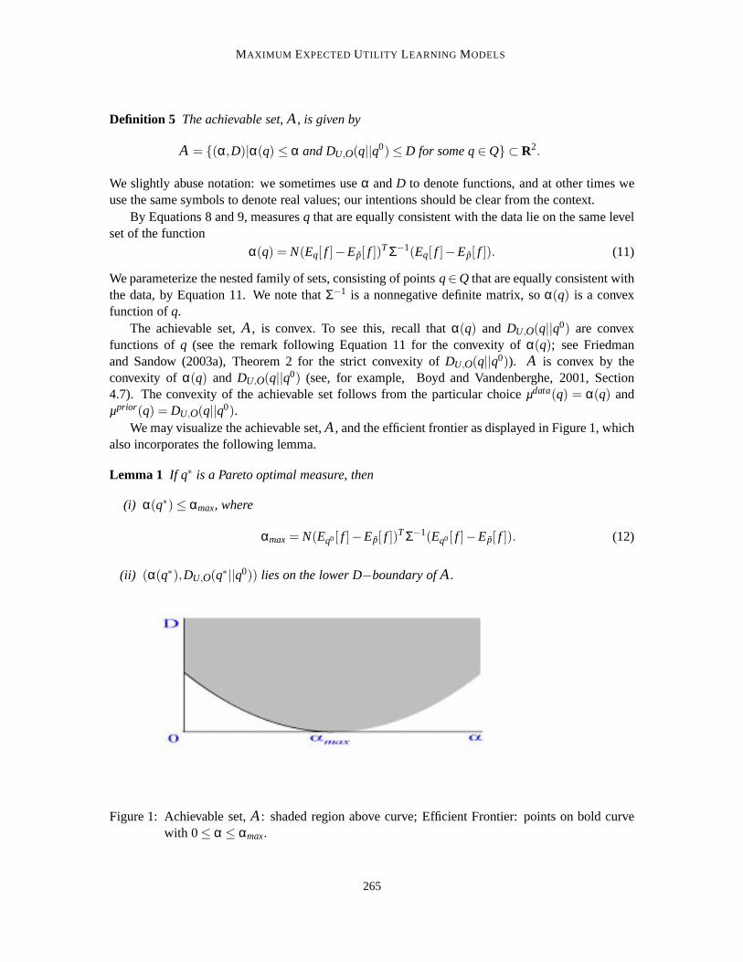
We may visualize the achievable set,A , and the efficient frontier as displayed in Figure 1, whichalso incorporates the following lemma.

Lemma 1 If q∗ is a Pareto optimal measure, then

(i) α(q∗)≤ αmax, where

αmax= N(Eq0[ f ]−Ep[ f ])TΣ−1(Eq0[ f ]−Ep[ f ]). (12)

(ii) (α(q∗),DU,O(q∗||q0)) lies on the lower D−boundary ofA .

Figure 1: Achievable set,A : shaded region above curve; Efficient Frontier: points on bold curvewith 0≤ α ≤ αmax.

265

FRIEDMAN AND SANDOW

Proof: (i) For the measureq0, we haveα(q0) = αmaxandD = DU,O(q0||q0) = 0. If α(q) > αmax,thenq cannot be identical toq0, soDU,O(q||q0) > 0, soq is dominated byq0 and cannot be efficient.(ii ) follows directly from Equation 10.�

We shall make use of the preceding lemma when we formulate our optimization problem.We make the following assumption, which serves as one of our guiding principles.

Assumption 4 The investor selects a measure on the efficient frontier.

Thus, given a set of measures equally consistent with the prior, our investor prefers measures thatare more consistent with the data, and, given a set of measures equally consistent with the data,he prefers measures that are more consistent with the prior. He makes no assumptions about theprecedence of these two preferences. We shall see (in Section 2.2.5) that every Pareto optimalmeasure is robust in the sense that it maximizes, over all measures, the worst-case (over measuresequally consistent with the data) relative outperformance of the model over the benchmark model.

2.2.4 CONVEX OPTIMIZATION PROBLEM

We seek the set of Pareto optimal measures. That is, motivated by Lemma 1, for allq ∈ Q withα(q) = α, we seek all solutions of the following problem, asα ranges from 0 toαmax, whereαmax

is defined in Equation 12.

Problem 1 (Initial Problem, Givenα,0≤ α ≤ αmax)

Find arg infq∈(R+)m,c∈RJ

DU,O(q||q0) (13)

under the constraints1 = ∑y

qy (14)

and NcTΣ−1c = α (15)

where cj = Eq[ f j ]−Ep[ f j ] . (16)

Problem 1 is not a standard convex optimization problem (see, for example, Berkovitz, 2002),since Equation 15 is a non-affine equality constraint. However, we formulate a different (strictlyconvex optimization) problem, which, as we shall show, has the same solutions:

Problem 2 (Initial Strictly Convex Problem, Givenα,0≤ α ≤ αmax)

Find arg minq∈(R+)m,c∈RJ

DU,O(q||q0) (17)


qy (18)

and NcTΣ−1c ≤ α (19)


Lemma 2 Problem 2 is a strictly convex optimization problem and Problems 1 and 2 have the sameunique solution.

266


Proof: See Appendix B.

In order to visualize the solutions to Problem 2, we define

Sα = {q : NcTΣ−1c = α,q∈Qc}, (21)

where

Qc = {q : q≥ 0,∑y

qy = 1,∑y

qy f j(y) = cj +Ep[ f j ], j = 1, . . . ,J}.

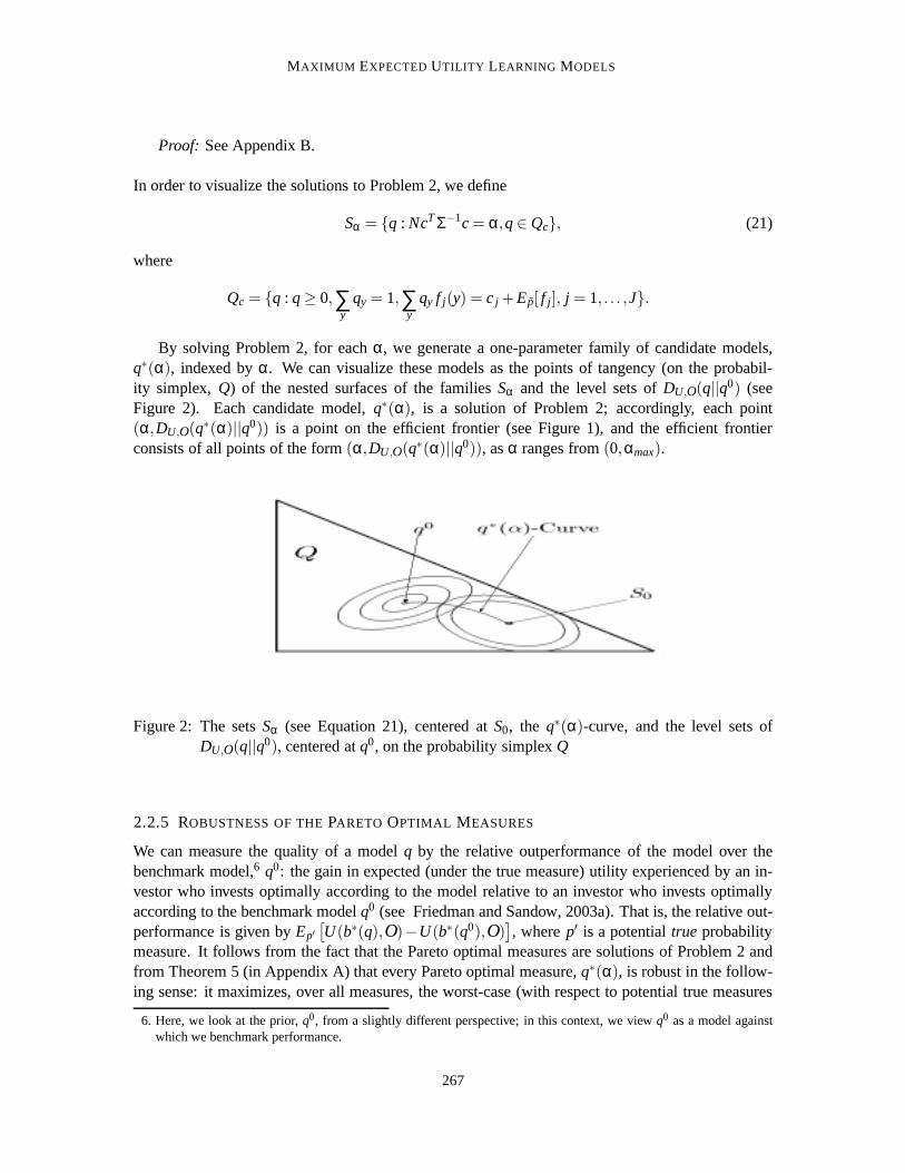
By solving Problem 2, for eachα, we generate a one-parameter family of candidate models,q∗(α), indexed byα. We can visualize these models as the points of tangency (on the probabil-ity simplex, Q) of the nested surfaces of the familiesSα and the level sets ofDU,O(q||q0) (seeFigure 2). Each candidate model,q∗(α), is a solution of Problem 2; accordingly, each point(α,DU,O(q∗(α)||q0)) is a point on the efficient frontier (see Figure 1), and the efficient frontierconsists of all points of the form(α,DU,O(q∗(α)||q0)), asα ranges from(0,αmax).

Figure 2: The setsSα (see Equation 21), centered atS0, the q∗(α)-curve, and the level sets ofDU,O(q||q0), centered atq0, on the probability simplexQ

2.2.5 ROBUSTNESS OF THEPARETO OPTIMAL MEASURES

We can measure the quality of a modelq by the relative outperformance of the model over thebenchmark model,6 q0: the gain in expected (under the true measure) utility experienced by an in-vestor who invests optimally according to the model relative to an investor who invests optimallyaccording to the benchmark modelq0 (see Friedman and Sandow, 2003a). That is, the relative out-performance is given byEp′

[U(b∗(q),O)−U(b∗(q0),O)

], wherep′ is a potentialtrue probability

measure. It follows from the fact that the Pareto optimal measures are solutions of Problem 2 andfrom Theorem 5 (in Appendix A) that every Pareto optimal measure,q∗(α), is robust in the follow-ing sense: it maximizes, over all measures, the worst-case (with respect to potential true measures

6. Here, we look at the prior,q0, from a slightly different perspective; in this context, we viewq0 as a model againstwhich we benchmark performance.

267

FRIEDMAN AND SANDOW

equally consistent with the data) relative outperformance of the model over the benchmark model,i.e.,

q∗(α) = argmaxq∈Q

minp′∈Sα

{Ep′ [U(b∗(q),O)]−Ep′

[U(b∗(q0),O)

]}.

2.2.6 CHOOSING A MEASURE ON THEEFFICIENT FRONTIER

According to our paradigm, the best candidate model lies on a one-parameter efficient frontier. Inorder to choose the best candidate model from this one-parameter family, we make the followingassumption.

Assumption 5 The investor choosesα so as to maximize his expected utility on an out-of-sampledata set.

Thus, given a utility function,U , odds ratios,O, and a prior belief,q0, Assumptions 1 to 5 leadto a method for finding a probability measure

q∗∗ = q∗(α∗) ,

with α∗ = argmaxα

Ep[U(b∗(q∗(α)),O)] ,

wherep is the empirical measure of the test set. In our method, the relative importance of the dataand the prior is determined by the out-of-sample performance (expected utility) of the model.

2.2.7 INFORMAL COMMENT: PRACTICAL BOUND FORα

In practice, given a confidence level,l , under Assumption 2, we can search over the range,

α ∈ (0,αsearch),

where

αsearch= min(αl ,αmax)

and

αl = (cd fχ2J)−1(l)

(see, for example, Davidson and MacKinnon, 1993 or Wu, 1997). That is, we search until

(i) we are 100· l% confident that the true value ofc is within the regionNcTΣ−1c≤ α,

(ii ) the regionNcTΣ−1c≤ α includesq0 andq∗ is insensitive to further increasing the value ofα.

In practice, the covariance matrixΣ may be nearly singular, so we may need to regularize it toinsure that our search spansc−space.

268


2.3 Dual Problem

We have shown in Section 2.2 that, in order to find the Pareto optimal model,q∗, for a givenα, wehave to solve Problem 2. As we have seen, this problem is strictly convex. Convex problems areknown to have so called dual problems.

We show in Appendix C that the dual of Problem 2 can be formulated as:

Problem 3 (Easily Interpreted Version of Dual Problem, Givenα)

Find β∗ = arg maxβ

h(β) (22)

with h(β) = ∑y

pyU(b∗y(q∗)Oy) −

√α

βTΣβN

, (23)

where b∗y(q∗) =

1Oy

(U ′)−1

(λ∗

q∗yOy

)(24)

and q∗y =λ∗

OyU ′ (U−1(Gy(q0,β,µ∗))), (25)

with Gy(q0,β,µ∗) = U(b∗y(q0)Oy) + βT f (y) − µ∗ , (26)

where µ∗ solves 1 = ∑y

1Oy

U−1(Gy(q0,β,µ∗))

, (27)

and λ∗ =

{∑y

1OyU ′ (U−1(Gy(q0,β,µ∗)))

}−1

. (28)

Equation 25 is often referred to as the connecting equation (see, for example, Lebanon andLafferty, 2001).

We also show in Appendix C that an alternative formulation of the dual problem is the following:

Problem 4 (Easily Implemented Version of Dual Problem, Givenα)


h(β) (29)

with h(β) = βTEp[ f ] − µ∗ −√

αβTΣβ

N, (30)


1Oy

U−1(Gy(q0,β,µ∗))

(31)

with Gy(q0,β,µ∗) = U(b∗y(q0)Oy) + βT f (y) − µ∗ . (32)

The optimal probability distribution is then

q∗y =λ∗

OyU ′ (U−1(Gy(q0,β∗,µ∗))), (33)

with λ∗ =

{∑y

1OyU ′ (U−1(Gy(q0,β∗,µ∗)))

}−1

. (34)

269

FRIEDMAN AND SANDOW

We state the following theorem:

Theorem 1 Problems 2, 3 and 4 have the same unique solution, q∗y.

Proof: see Appendix C.

Problems 3 and 4 are equivalent. Problem 4 is easier to implement and Problem 3 is easier tointerpret. The first term in the objective function of Problem 3 is the utility (of the utility maximizinginvestor) averaged over the training sample. Thus, our dual problem is a regularized maximizationof the training-sample averaged utility, where the utility function,U , is the utility function on whichthe generalized relative entropyDU,O(q||q0) depends.

The dual problems, Problems 3 and 4, areJ-dimensional (J is the number of features), un-constrained, concave maximization problems (see Boyd and Vandenberghe, 2001, p. 159 for theconcavity). The primal problem, Problem 2, on the other hand, is anm-dimensional (m is the num-ber of states) convex minimization with convex quadratic constraints. The dual problem, Problem4, may be easier to solve than the primal problem, Problem 2, ifm> J. In the more general contextdiscussed in section 3, the dual problem will always be easier to solve than the primal problem.

We note that we can obtain the sameα−parameterized family of solutions to Problems 3 and4, if we allowα to vary over[0,∞), by dropping the square roots in Equations 23 and 30; we showthat this is so in Appendix E.

2.3.1 ASYMPTOTIC OPTIMALITY

It follows from Equation 23 that

Theorem 2 As N→ ∞, to leading order, the optimal solution to Problem 2 maximizes (over theparametric family prescribed by the connecting equation, Equation 25) the expected utility for theinvestor.

2.3.2 EXAMPLE: A L OGARITHMIC FAMILY OF UTILITIES

We consider a utility of the form

U(z) = γ1log(z+ γ)+ γ2 , γ >− 1

∑y1

Oy

, γ1 > 0 , (35)

(see Theorems 3 and 4 in Friedman and Sandow, 2003a). This logarithmic family is rich enoughto describe a wide range of risk aversions; and it can be used to approximate non-logarithmic utilityfunctions (see Friedman and Sandow, 2003a).

In Appendix D, we show that the dual problem is given by:

Problem 5 (Dual Problem for our Logarithmic Family of Utilities)


h(β)

with h(β) = ∑y

py logq∗y −√

αγ2

1

βTΣβN

,

where q∗y =1

∑yq0yeβT f (y)

q0y eβT f (y) .

270


This problem is equivalent to a regularized maximum likelihood search, which is independentof the odds ratios,O; this is consistent with Section 2.5, where we show that the odds ratios dropout of the primal problem for this logarithmic family of utility functions.

2.3.3 EXAMPLE: POWER UTILITY

We consider a utility of the form

U(z) =z1−κ−1

1−κ. (36)

(see Section 2.1.1 in Friedman and Sandow, 2003a). In order to specify the dual problem for thisutility, note that

U ′(z) = z−κ , (37)

U−1(z) = [1+(1−κ)z]1

1−κ (38)

andU ′(U−1(z)) = [1+(1−κ)z]−κ1−κ . (39)

One can show that

b∗(q) =(qyOy)

1κ

OyB(q,O)(40)

with B(q,O) = ∑y

1Oy

(qyOy)1κ , (41)

(see Section 2.1.1 in Friedman and Sandow, 2003a). Using this equation, we can writeGy(q0,β,µ∗)from Equation 26 as

Gy(q0,β,µ∗) =1

1−κ

[((q0

yOy)1−κ

κ

(B(q0,O))1−κ

)−1

]+ βT f (y) − µ∗ . (42)

Inserting Equations 38 and 42 into Equation 27 gives

1 = ∑y

1Oy

[(q0

yOy)1−κ

κ

(B(q0,O))1−κ +(1−κ)[βT f (y)−µ∗]

] 11−κ

, (43)

which is our condition forµ∗. Next we specify the condition Equation 28 forλ∗. We use Equations39 and 42 to write Equation 28 as

λ∗ =

∑

y

1Oy

[(q0

yOy)1−κ

κ

(B(q0,O))1−κ +(1−κ)[βT f (y)−µ∗]

] κ1−κ−1

. (44)

By means of Equations 25, 39 and 42 we obtain for the optimal probability distribution

q∗y =1

Oy

[(q0

yOy)1−κ

κ

(B(q0,O))1−κ +(1−κ)[βT f (y)−µ∗]

] κ1−κ

. (45)

Collecting Equations 43, 41, 44 and 45, we obtain:

271

FRIEDMAN AND SANDOW

Problem 6 (Dual problem for power utility)


h(β)

with h(β) = βTEp[ f ] − µ∗ −√

αβTΣβ

N,


1Oy

[(q0

yOy)1−κ

κ

(B(q0,O))1−κ +(1−κ)[βT f (y)−µ∗]

] 11−κ

with B(q0,O) = ∑y

1Oy

(q0yOy)

1κ .

The optimal probability distribution is then

q∗y =λ∗

Oy

[(q0

yOy)1−κ

κ

(B(q0,O))1−κ +(1−κ)[β∗T f (y)−µ∗]

] κ1−κ

with λ∗ =

∑

y

1Oy

[(q0

yOy)1−κ

κ

(B(q0,O))1−κ +(1−κ)[β∗T f (y)−µ∗]

] κ1−κ−1

2.4 Summary of Modeling Approach

The modeling approach described in Sections 2.2 and 2.3 is based on the idea that our investorselects a Pareto optimal model, i.e. a model on an efficient frontier, which we have defined in termsof consistency with the training data and consistency with a prior distribution. We measured theformer by means of the large-sample distribution of a vector of sample-averaged features, and thelatter by means of a generalized relative entropy. We have seen that the measures on the efficientfrontier form a family which is parameterized by the single parameterα ∈ (0,αmax), and that, for agivenα, the Pareto optimal measure is the unique solution of Problem 2, which is a strictly convexoptimization problem. Moreover, the Pareto optimal measures are robust in the sense of Theorem 5.For a givenα, the Pareto optimal measure can be found by solving the dual (concave maximization)problem in the form of Problem 3 or in the form of Problem 4. Solving this dual problem amountsto a regularized expected utility maximization (over the training sample) over a certain family ofmeasures; for many practical examples, solving the dual problem can be easier than solving theprimal problem. Having thus computed anα-parameterized family of Pareto optimal measures, wepick the measure with highest expected utility on a hold-out sample.

We note that the procedure to selectα is, by virtue of the fact thatα is one-dimensional, bothtractable and barely susceptible to overfitting on the hold-out sample set.

Our approach boils down to the following procedure:

272


1. Break the data into a training set and a hold-out sample. (In their numerical experiments,Friedman and Sandow, 2003b, Friedman and Huang, 2003, and Sandow et al., 2003 used75% or 80% of the data, selected randomly, to train the model.)

2. Choose a discrete setA = {αk ∈ (0,αmax),k = 1, . . . ,K}.3. Fork = 1, . . . ,K,

• Solve Problem 4 forβ∗(αk), based on the training set,

• Compute the out-of-sample performancePk = Ep[U(b∗(q∗(αk)),O)] on the out-of-sample test set, where ˜p is the empirical measure on this test set, andq∗, is determinedfrom Equation 33 with parametersβ∗(αk), andb∗ is determined from Equation 3.

4. Putk∗ = argmaxk Pk.

5. Our model,q∗∗, is determined from Equation 33 with parametersβ∗(αk∗).

2.5 Utilities Admitting Odds Ratio Independent Problems: a Logarithmic Family

Model builders who use probabilistic models make decisions (bets) which result in well definedbenefits or ill effects (payoffs) in the presence of risk. In principle, the payoffs associated withthe various outcomes can be assigned precise values; in practice, it may be difficult to assign suchvalues. Outside the financial modeling context, for example, there may be no “market makers” whoset odds ratios. Even in the financial modeling context, the data for the payoffs (or equivalently,market prices or odds ratios) may not exist or be of poor quality. In this context, given market priceson instruments which have nonzero payoffs for more than one state, we would need a completemarket in order to calculate the odds ratios (see, for example, Duffie, 1996, for a definition ofcomplete markets). In the absence of high quality data, one might consider modeling the oddsratios, but that introduces additional complexity; moreover, the resulting model, under a generalutility function, will be sensitive to the odds ratio model.

For these reasons, we seek the most general family of utility functions for which our problemformulation is independent of the odds ratios. This family is specified in the following theorem

Theorem 3 The generalized relative entropy, DU,O(q||q0), is independent of the odds ratios,O, forany candidate model q and prior measure, q0, if and only if the utility function, U, is a member ofthe logarithmic family

U(W) = γ1 log(W + γ)+ γ2 , ∀W > max{0,−γ} , (46)

whereγ1 > 0, γ2 andγ >− 1∑y

1Oy

are constants. In this case,

DU,O(q||q0) = γ1Eq

[log

(qq0

)], (47)

which depends onγ1 in a trivial way and is independent ofγ andγ2.

273

FRIEDMAN AND SANDOW

Proof: First we prove that if the utility function has the form Equation 46 thenDU,O(q||q0)is independent ofO, for any measuresq andq0, and Equation 47 holds. Theorem 4 in Friedmanand Sandow (2003a) states that, if the utility function has the form Equation 46 then the relativeperformance measure7

∆U(q1,q2,O) = ∑y

py[U(b∗y(q2)Oy)−U(b∗y(q

1)Oy)] (48)

is independent ofO, for any measuresq1,q2, and p. Puttingp= q, q1 = q0 andq2 = q, we see fromEquations 48 and 6 that

DU,O(q||q0) = ∆U(q1,q2,O) .

It follows from Theorem 4 in Friedman and Sandow (2003a) that

DU,O(q||q0) = γ1Eq

[log

(qq0

)],

which is independent ofO, for any measuresq andq0.Next we prove the reverse: IfDU,O(q||q0) is independent ofO, for any measuresq, andq0, then

the utility function has the form Equation 46. IfDU,O(q||q0) is independent ofO, for any measuresq andq0, then bothDU,O(p||q1) andDU,O(p||q2) are independent ofO, for any measures ˜p,q1 andq2. Consequently, the performance measure

∆U(q1,q2,O) = DU,O(p||q1)−DU,O(p||q2)

is independent ofO, for any measures ˜p,q1 andq2. It follows then from Theorem 3 in Friedmanand Sandow (2003a) that the utility function has the form Equation 46.�

From this theorem and Problem 2, we obtain

Corollary 1 For utility functions of the form Equation 35, Problem 2 reduces to Problem 7.

Problem 7 (Initial Strictly Convex Problem for U in our Logarithmic Family, Givenα,0≤ α ≤αmax)

Find arg minq∈(R+)m,c∈RJ

γ1Eq

[log

(qq0

)]under the constraints1 = ∑

yqy

and NcTΣ−1c ≤ αwhere cj = Eq[ f j ]−Ep[ f j ] .

We have already explicitly derived the dual problem for utility functions of the form Equation46 in Section 2.3.2.

We note that the family of utility functions Equation 46 admits a wide range of risk aversions(see the discussion in Friedman and Sandow, 2003a, Section 2.3). Moreover, for utilities not ofthis form and horse races with sufficiently homogeneous expected returns, we can approximate wellDU,O(q||q0) by Dlog,O(q||q0); see Friedman and Sandow (2003a), Theorem 5. For utilities in thislogarithmic family, the primal problem (Problem 2) and equivalent dual problems (Problems 3 and4) are independent of the odds ratios.

7. Modelq2 outperforms modelq1 if and only if ∆U (q1,q2,O) > 0.

274


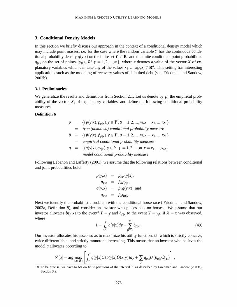
3. Conditional Density Models

In this section we briefly discuss our approach in the context of a conditional density model whichmay include point masses, i.e. for the case where the random variableY has the continuous condi-tional probability densityq(y|x) on the finite setY ⊂Rn and the finite conditional point probabilitiesqρ|x on the set of points{yρ ∈ Rn,ρ = 1,2, ...,m}, wherex denotes a value of the vectorX of ex-planatory variables which can take any of the valuesx1, ...,xM ,xi ∈ Rd. This setting has interestingapplications such as the modeling of recovery values of defaulted debt (see Friedman and Sandow,2003b).

3.1 Preliminaries

We generalize the results and definitions from Section 2.1. Let us denote by ˜px the empirical prob-ability of the vector,X, of explanatory variables, and define the following conditional probabilitymeasures:

Definition 6

p = {(p(y|x), pρ|x),y∈ Y ,ρ = 1,2, ...,m,x = x1, ...,xM}= true (unknown) conditional probability measure

p = {(p(y|x), pρ|x),y∈ Y ,ρ = 1,2, ...,m,x = x1, ...,xM}= empirical conditional probability measure

q = {(q(y|x),qρ|x),y∈ Y ,ρ = 1,2, ...,m,x = x1, ...,xM}= model conditional probability measure

Following Lebanon and Lafferty (2001), we assume that the following relations between conditionaland joint probabilities hold:

p(y,x) = pxp(y|x),pρ,x = pxpρ|x,

q(y,x) = pxq(y|x), and

qρ,x = pxqρ|x.

Next we identify the probabilistic problem with the conditional horse race ( Friedman and Sandow,2003a, Definition 8), and consider an investor who places bets on horses. We assume that ourinvestor allocatesb(y|x) to the event8 Y = y andbρ|x to the eventY = yρ, if X = x was observed,where

1 =∫

Yb(y|x)dy+

m

∑ρ=1

bρ|x . (49)

Our investor allocates his assets so as to maximize his utility function,U , which is strictly concave,twice differentiable, and strictly monotone increasing. This means that an investor who believes themodelq allocates according to

b∗[q] = arg max{b∈B}

[∫Y

q(y|x)U(b(y|x)O(x,y))dy+∑y

qρ|xU(bρ|xOx,ρ)

],

8. To be precise, we have to bet on finite partitions of the intervalY as described by Friedman and Sandow (2003a),Section 3.2.

275

FRIEDMAN AND SANDOW

where

B = {(b(y|x),bρ|x) :∫

Yb(y|x)dy+

m

∑ρ=1

bρ|x = 1}′

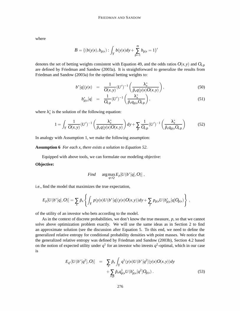
denotes the set of betting weights consistent with Equation 49, and the odds ratiosO(x,y) andOx,ρare defined by Friedman and Sandow (2003a). It is straightforward to generalize the results fromFriedman and Sandow (2003a) for the optimal betting weights to:

b∗[q](y|x) =1

O(x,y)(U ′)−1

(λ∗x

pxq(y|x)O(x,y)

), (50)

b∗ρ|x[q] =1

Ox,ρ(U ′)−1

(λ∗x

pxqρ|xOx,ρ

), (51)

whereλ∗x is the solution of the following equation:

1 =∫

Y

1O(x,y)

(U ′)−1(

λ∗xpxq(y|x)O(x,y)

)dy+∑

ρ

1Ox,ρ

(U ′)−1(

λ∗xpxqρ|xOx,ρ

)(52)

In analogy with Assumption 1, we make the following assumption:

Assumption 6 For each x, there exists a solution to Equation 52.

Equipped with above tools, we can formulate our modeling objective:

Objective:

Find argmaxq∈Q

Ep[U(b∗[q],O)] ,

i.e., find the model that maximizes the true expectation,

Ep[U(b∗[q],O)] = ∑x

px

{∫Y

p(y|x)U(b∗[q](y|x)O(x,y))dy+∑y

pρ|xU(b∗ρ|x[q]Oρ|x)

},

of the utility of an investor who bets according to the model.As in the context of discrete probabilities, we don’t know the true measure,p, so that we cannot

solve above optimization problem exactly. We will use the same ideas as in Section 2 to findan approximate solution (see the discussion after Equation 5. To this end, we need to define thegeneralized relative entropy for conditional probability densities with point masses. We notice thatthe generalized relative entropy was defined by Friedman and Sandow (2003b), Section 4.2 basedon the notion of expected utility underq1 for an investor who investsq2-optimal, which in our caseis

Eq1[U(b∗[q2],O)] = ∑x

px

∫Y

q1(y|x)U(b∗[q2](y|x)O(x,y))dy

+∑x,ρ

pxq1ρ|xU(b∗ρ|x[q

2]Oρ|x) . (53)

276


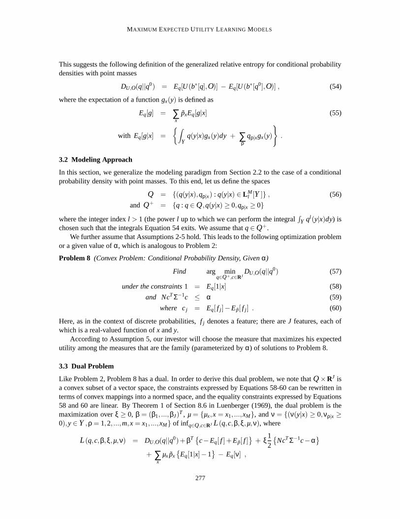
This suggests the following definition of the generalized relative entropy for conditional probabilitydensities with point masses

DU,O(q||q0) = Eq[U(b∗[q],O)] − Eq[U(b∗[q0],O)] , (54)

where the expectation of a functiongx(y) is defined as

Eq[g] = ∑x

pxEq[g|x] (55)

with Eq[g|x] ={∫

Yq(y|x)gx(y)dy + ∑

ρqρ|xgx(y)

}.

3.2 Modeling Approach

In this section, we generalize the modeling paradigm from Section 2.2 to the case of a conditionalprobability density with point masses. To this end, let us define the spaces

Q = {(q(y|x),qρ|x) : q(y|x) ∈ LMl [Y ]} , (56)

and Q + = {q : q∈ Q ,q(y|x) ≥ 0,qρ|x ≥ 0}where the integer indexl > 1 (the powerl up to which we can perform the integral

∫Y ql (y|x)dy) is

chosen such that the integrals Equation 54 exits. We assume thatq∈ Q +.We further assume that Assumptions 2-5 hold. This leads to the following optimization problem

or a given value ofα, which is analogous to Problem 2:

Problem 8 (Convex Problem: Conditional Probability Density, Givenα)

Find arg minq∈Q +,c∈RJ

DU,O(q||q0) (57)

under the constraints1 = Eq[1|x] (58)



Here, as in the context of discrete probabilities,f j denotes a feature; there areJ features, each ofwhich is a real-valued function ofx andy.

According to Assumption 5, our investor will choose the measure that maximizes his expectedutility among the measures that are the family (parameterized byα) of solutions to Problem 8.

3.3 Dual Problem

Like Problem 2, Problem 8 has a dual. In order to derive this dual problem, we note thatQ ×RJ isa convex subset of a vector space, the constraints expressed by Equations 58-60 can be rewritten interms of convex mappings into a normed space, and the equality constraints expressed by Equations58 and 60 are linear. By Theorem 1 of Section 8.6 in Luenberger (1969), the dual problem is themaximization overξ ≥ 0, β = (β1, ...,βJ)T , µ = {µx,x = x1, ...,xM}, andν = {(ν(y|x) ≥ 0,νρ|x ≥0),y∈ Y ,ρ = 1,2, ...,m,x = x1, ...,xM} of infq∈Q ,c∈RJ L(q,c,β,ξ,µ,ν), where

L(q,c,β,ξ,µ,ν) = DU,O(q||q0)+ βT {c−Eq[ f ]+Ep[ f ]}

+ ξ12

{NcTΣ−1c−α

}+ ∑

xµxpx

{Eq[1|x]−1

} − Eq[ν] ,

277

FRIEDMAN AND SANDOW

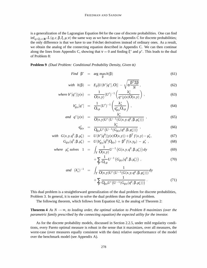
is a generalization of the Lagrangian Equation 84 for the case of discrete probabilities. One can findinfq∈Q ,c∈RJ L(q,c,β,ξ,µ,ν) the same way as we have done in Appendix C for discrete probabilities;the only difference is that we have to use Fréchet derivatives instead of ordinary ones. As a result,we obtain the analog of the connecting equation described in Appendix C. We can then continuealong the lines from Appendix C, showing thatν = 0 and findingξ∗ andµ∗. This leads to the dualof Problem 8:

Problem 9 (Dual Problem: Conditional Probability Density, Givenα)


h(β) (61)

with h(β) = Ep[U(b∗[q∗],O)] −√

αβTΣβ

N, (62)

where b∗[q∗](y|x) =1

O(x,y)(U ′)−1

(λ∗x

q∗(y|x)O(x,y)

), (63)

b∗ρ|x[q∗] =

1Ox,ρ

(U ′)−1

(λ∗x

q∗ρ|xOx,ρ

), (64)

and q∗(y|x) =λ∗x

O(x,y)U ′ (U−1(G(x,y,q0,β,µ∗x))), (65)

q∗ρ|x =λ∗x

Oρ|xU ′ (U−1(Gρ|x(q0,β,µ∗x))) , (66)

with G(x,y,q0,β,µ∗x) = U(b∗[q0](y|x)O(x,y))+ βT f (x,y)−µ∗x, (67)

Gρ|x(q0,β,µ∗x) = U(b∗ρ|x[q0]Oρ|x) + βT f (x,yρ) − µ∗x , (68)

where µ∗x solves 1 =∫

Y

1O(x,y)

U−1(G(x,y,q0,β,µ∗x))

dy (69)

+∑ρ

1Ox,ρ

U−1(Gρ|x(q0,β,µ∗x))

, (70)

and (λ∗x)−1 =

∫Y

1O(x,y)U ′ (U−1(G(x,y,q0,β,µ∗x)))

dy

+∑ρ

1

Oρ|xU ′ (U−1(Gρ|x(q0,β,µ∗x))) . (71)

This dual problem is a straightforward generalization of the dual problem for discrete probabilities,Problem 3. In general, it is easier to solve the dual problem than the primal problem.

The following theorem, which follows from Equation 62, is the analog of Theorem 2:

Theorem 4 As N→ ∞, to leading order, the optimal solution to Problem 8 maximizes (over theparametric family prescribed by the connecting equation) the expected utility for the investor.

As for the discrete probability models, discussed in Section 2.2.5, under mild regularity condi-tions, every Pareto optimal measure is robust in the sense that it maximizes, over all measures, theworst-case (over measures equally consistent with the data) relative outperformance of the modelover the benchmark model (see Appendix A).

278


We note that we can obtain the sameα−parameterized family of solutions to Problem 10, if weallow α to vary over[0,∞), by dropping the square root in Equation 75; we show that this is so inAppendix E.

3.3.1 EXAMPLE: UTILITIES FROM OUR LOGARITHMIC FAMILY

Because of its practical relevance, we state the above dual problem for the case of a utility fromthe logarithmic family Equation 35. It is easy to see that, in this case, the Equations 50-52 for theoptimal betting weights give:

b∗ρ|x[q] = qρ|x

[1+ γ∑

ρ′

1Ox,ρ′

]− γ

Ox,ρ(72)

b∗[q](y|x) = q(y|x)[

1+ γ∑y′

1O(x,y′)

]− γ

O(x,y). (73)

The generalized relative entropy, which enters Problem 8, is then

DU,O(q||q0) = γ1Eq

[log

(qq0

)]. (74)

Inserting Equations 35, 72 and 73 into Problem 9, we derive the dual problem as:

Problem 10 (Dual Problem for Probability Densities and our Logarithmic Family of Utilities)


h(β)

with h(β) =1N ∑

ilogq(β)(yi |xi) −

√αγ2

1

βTΣβN

, (75)

where q(β)(y|x) = Z−1x eβT f (x,y) ×

{q0

ρ|x if y = yρ for someρq0(y|x) otherwise,

(76)

and Zx =∫

Yq0(y|x)eβT f (x,y)dy + ∑

ρq0

ρ|xeβT f (x,yρ) , (77)

where the(xi ,yi) are the observed values andN is the number of observations. The measure on theefficient frontier is then

q∗ = {(q∗(y|x),q∗ρ|x),y∈ Y ,ρ = 1,2, ...,m,x = x1, ...,xM}with q∗(y|x) = q(β∗)(y|x)

and q∗ρ|x = q(β∗)(yρ|x) .

We note that we can obtain the sameα−parameterized family of solutions to Problem 10, if weallow α to vary over[0,∞), by dropping the square root in Equation 75; we show that this is so inAppendix E.

3.3.2 EXAMPLE: LOGISTIC REGRESSION

We note that in the special case whereU(W) is in our logarithmic family Equation 35,Y = /0, m= 2,the prior is flat, andα = 0, the dual problem, Problem 10, is the logistic regression problem.

279

FRIEDMAN AND SANDOW

3.4 Summary of Modeling Approach

The logic of our modeling approach in this section’s more general context is similar to the logicdescribed in Section 2.4. We have the following procedure:

1. Break the data into a training set and a hold-out sample. (In their numerical experiments,Friedman and Sandow, 2003b, Friedman and Huang, 2003, and Sandow et al., 2003) used75% or 80% of the data, selected randomly, to train the model.)

2. Choose a discrete setA = {αk ∈ (0,αmax),k = 1, . . . ,K}.3. Fork = 1, . . . ,K,

• Solve Problem 9 forβ∗(αk),

• Compute the out-of-sample performancePk = Ep[U(b∗(q∗(αk)),O)] on the out-of-sample test set, where ˜p is the empirical measure on this test set, andq∗, is determinedfrom Equations 65 and 66 with parametersβ∗(αk), andb∗ is determined from Equations63 and 64.

4. Putk∗ = argmaxk Pk.

5. Our model,q∗∗, is determined from Equations 65 and 66 with parametersβ∗(αk∗).

Acknowledgments

We thank Max Chickering, James Huang and an anonymous referee for their insightful comments.

Appendix A. Robustness of the Minimum Generalized Relative Entropy Measure

In this appendix, we state and prove the following theorem, which is only a slight modification of aresult from Grunwald and Dawid (2002) and is based on the logic from Topsøe (1979).

Theorem 5

argminq∈K

DU,O(q||q0) = argmaxq∈Q

minp′∈K

{Ep′ [U(b∗(q),O)]−Ep′

[U(b∗(q0),O)

]},

where Q is the compact convex set of all possible probability measures, and K⊂Q is compact andconvex.

Interpretation: We can measure the quality of a modelq by the gain in expected (under the truemeasure) utility experienced by an investor who invests optimally according to the model relative toan investor who invests optimally according to the benchmark modelq0 (see Friedman and Sandow,2003a), i.e. byEp′

[U(b∗(q),O)−U(b∗(q0),O)

], wherep′ is thetrueprobability measure. If we use

this performance measure, Theorem 5 states the following: minimizingDU,O(q||q0) with respect toq∈ K is equivalent to searching for the measureq∗ ∈Q that maximizes the worst-case (with respect

280


to the potential true measures,p′ ∈ K) relative model performance. The optimal model,q∗, is robustin the sense that for any other model,q, the worst (over potential true measuresp′ ∈ K) relativeperformance is even worse than the worst-case relative performance underq∗. We do not know thetrue measure; an investor who makes allocation decisions based onq∗ is prepared for the worst thatnature can offer.

Proof: We start with the definition, Equation 6, of the generalized relative entropy:

DU,O(q||q0) = Eq [U(b∗(q),O)]−Eq[U(b∗(q0),O)

].

By the definition (Equation 2) of the optimal betting weights,b∗,

Eq [U(b∗(q),O)] ≥ Eq [U(b∗(π),O)] , (78)

for any measureπ ∈Q. Therefore, we have

DU,O(q||q0) = maxπ∈Q

{Eq [U(b∗(π),O)]−Eq

[U(b∗(q0),O)

]},

and

minq∈K

DU,O(q||q0) = minq∈K

maxπ∈Q


[U(b∗(q0),O)

]}.

Since bothK andQ are compact and convex, andEq[U(b∗(π),O)−U(b∗(q0),O)

]is a continuous

concave-convex function onK×Q, we can apply a minimax theorem (see, for example, Frenket al., 2002, Theorem 3); we obtain

minq∈K

DU,O(q||q0) = maxπ∈Q

minq∈K


[U(b∗(q0),O)

]}.

The maximum is attained for some pair,(π∗,q∗). From Equation 78, it follows thatπ∗ = q∗. To seethis, suppose thatπ∗ 6= q∗; then, withq∗ fixed, we can increase the value of the term{

Eq∗ [U(b∗(π∗),O)]−Eq∗[U(b∗(q0),O)

]}by settingπ∗ = q∗, which contradicts our assumption that the maximum is attained for the pair(π∗,q∗) with π∗ 6= q∗. So

argminq∈K

DU,O(q||q0) = argmaxπ∈Q

minq∈K


[U(b∗(q0),O)

]}.

After renaming the optimization variables of the right-hand-side:q as p′ and π as q, we obtainTheorem 5.�.

We note that this result can be applied directly to the discrete probability case (see Section2.2.5). For conditional density models, we restrict the admissible probability measures so thatthe maximum value of the probability density is less than some finite number,qmax, to insure thecompactness ofK in the preceding theorem. We can always do so without changing the Paretooptimal measure by choosing

qmax= a·maxx,y

q∗(y|x),

wherea> 1 is some constant andq∗(y|x) is given in Equation 65. Note that any measure inQ + canbe approximated by a measure inK for a sufficiently large, and thatq∗(y|x) is finite for all utilities.

281

FRIEDMAN AND SANDOW

Appendix B. Proof of Lemma 2

We restate Lemma 2:Lemma 2Problem 2 is a strictly convex optimization problem and Problems 1 and 2 have the sameunique solution.

Proof: We note that the objective function,DU,O(q||q0), is strictly convex (see Theorem 2 inFriedman and Sandow, 2003a). The inequality constraint, Inequality 19, of Problem 2 is also con-vex; this follows from the fact thatΣ is a covariance matrix and therefore nonnegative definite. Theequality constraints, Equations 18 and 20, are both affine. Therefore, Problem 2 is a strictly convexprogramming problem (see, for example, the Convex Programming Problem II Berkovitz, 2002).

We now show that Problems 1 and 2 have the same unique solution.We firstassume thatα < αmax, and show that in this case, the solution to Problem 2 satisfies

NcTΣ−1c = α.

To this end, we note thatDU,O(q||q0) is strictly convex inq, for q in the simplexQ, and that theglobal minimum of the functionDU,O(q||q0) occurs atq = q0 (see Friedman and Sandow, 2003a,Theorem 2 for theseDU,O(q||q0) properties), which occurs only ifα = αmax; therefore,

∇qDU,O(q||q0) 6= 0 (79)

for q 6= q0. Suppose thatq∗ is such thatNc(q∗)TΣ−1c(q∗) < α where

c(q) = Eq[ f ]−Ep[ f ].

Then there exists a neighborhood ofq∗ on the simplexQ, such that for allq in the neighborhood,Nc(q)TΣ−1c(q)≤ α. From Equation 79, we see that there is a direction of decrease of the objectivefunctionDU,O(q||q0) on the simplexQ, soq∗ cannot be the optimal solution. Therefore, we cannothaveNc(q∗)TΣ−1c(q∗) < α. It follows that NcTΣ−1c = α, so the solution to Problem 2 is thesolution to 1 for the caseα < αmax.

In the caseα = αmax, it is obvious that both problems have the unique solutionq∗ = q0.The objective function,DU,O(q||q0) is strictly convex inq, so the solution of Problem 2 is unique

(see, for example, Rockafellar, 1970, Section 27). It follows that the solution to Problem 1 is alsounique.�

Appendix C. Proof of Theorem 1

We will show that Problem 2, which we restate below for convenience, has the (equivalent) dualformulations Problems 3 and 4.

Problem 2 (Initial Convex Problem, Givenα,0≤ α ≤ αmax)

Find minq∈(R+)m,c∈RJ

DU,O(q||q0) (80)


qy (81)



282


We will derive the dual of Problem 2 now. To this end, note that the Lagrangian is given by

L(q,c,β,ξ,µ,ν) = DU,O(q||q0)+ βT {c−Eq[ f ]+Ep[ f ]}

+ξ12

{NcTΣ−1c−α

}+ µ

{∑y

qy−1

}

−νTq, (84)

whereξ ≥ 0, β = (β1, ...,βJ)T , µ, andνT = (ν1, . . . ,νm) ≥ 0 are Lagrange multipliers andq variesoverRm.

C.1 The Connecting Equation

In order to derive the connecting equation, we have to solve

0 =∂L(q,c,β,ξ,µ,ν)

∂cj(85)

and 0 =∂L(q,c,β,ξ,µ,ν)

∂qy. (86)

The first one of these equations has solution

c = c∗ ≡ − 1ξN

Σβ . (87)

In order to solve Equation 86, we insert Equation 84 and the equation (see Lemma 2 from Friedmanand Sandow, 2003a)

∂DU,O(q||q0)∂qy

= U(b∗y(q)Oy)−U(b∗y(q0)Oy) , (88)

into Equation 86, and obtain

0 = U(b∗y(q)Oy)−U(b∗y(q0)Oy) − βT f (y) + µ−νy . (89)

We rewrite this equation as

U(b∗y(q)Oy) = Gy(q0,β,µ,ν) (90)

with Gy(q0,β,µ,ν) = U(b∗y(q0)Oy) + βT f (y) − µ+ νy , (91)

whereGy(q0,β,µ,ν) does not depend onq. In order to solve forq, we substitute Equation 3 intoEquation 90, to obtain

U

(U ′−1

(λ

qyOy

))= Gy(q0,β,µ,ν) . (92)

Solving forqy, we obtain the connecting equation

q∗y ≡λ

OyU ′ (U−1(Gy(q0,β,µ,ν))). (93)

283

FRIEDMAN AND SANDOW

From Equation 93, by the positivity of theOy and the fact theU is a monotone increasingfunction, we conclude that all of theq∗y andλ have the same sign. We note, from Equation 81, thattheq∗y andλ must be positive. From the Karush-Kuhn-Tucker conditions, we must haveνyq∗y = 0;it follows thatν∗y = 0 for all y. Accordingly, we may suppress the dependence ofG andL on ν.

The connecting equation, Equation 93, depends onβ,λ, andµ. We now show how to calculate

λ andµ in terms ofβ. Solving Equation 92 forU ′−1(

λqyOy

)and substituting into Equation 4, we

obtain a condition forµ∗:

∑y

1Oy

U−1(Gy(q0,β,µ∗))

= 1 . (94)

This equation is easy to solve numerically forµ∗, by the following lemma.

Lemma 3 There exists a unique solution, µ∗, to Equation 94. The left hand side of Equation 94 isa strictly monotone decreasing function of µ∗.

Proof: First, we note that sinceU is a strictly increasing function,

(U−1)′ =1

dUdW

> 0,

soU−1 is a strictly increasing function and the left hand side of Equation 94 is a strictly decreasingfunction ofµ∗.

Letting

µ= maxy

βT f (y),

we see that

βT f (y)−µ≤ 0 for all y.

In this case, it follows from Equation 91 that

Gy(q0,β,µ)≤U(b∗y(q0)Oy) for all y,

so, by the monotonicity ofU−1,

∑y

1Oy

U−1(Gy(q0,β,µ)) ≤ ∑

y

1Oy

U−1(U(b∗y(q0)Oy)

)(95)

= ∑y

b∗y(q0) = 1.

Note thatGy(q0,β,µ) ∈ dom(U−1) for all y, by Equation 90. Similarly, by letting

µ= miny

βT f (y),

we can guarantee that

∑y

1Oy

U−1(Gy(q0,β,µ))≥ 1.

284


By the Intermediate Value Theorem and the monotonicity and continuity of the left hand side ofEquation 94, there exists a unique solution to Equation 94.�

We now show how to calculateλ in terms ofβ andµ∗. We insert Equation 93 into Equation 81,and obtain:

1 = λ∑y

1OyU ′ (U−1(Gy(q0,β,µ∗)))

;

solving forλ, we obtain

λ∗ ≡{

∑y

1OyU ′ (U−1(Gy(q0,β,µ∗)))

}−1

. (96)

Summarizing the result of this subsection:

The connecting equation, which describesq∗ as a member of a parametric fam-ily (in β), is given by

q∗y =λ∗

OyU ′ (U−1(Gy(q0,β,µ∗))), (97)

where we determineµ∗ from Equation 94 via Lemma 3 andλ∗ from Equation96.

C.2 Dual Problems

We now show that

Lemma 4 Problem 4 is the dual of Problem 2.

Proof: Equations 87 and 93, together with the Equations 94 and 96, give the vectorc∗, theprobabilitiesq∗y and the Lagrange multipliersµ∗,ν∗ for which the Lagrangian is at its minimum forgiven multipliersβ,ξ. This allows us to formulate the dual problem as an optimization with respectto β andξ. To this end, we have to computeL(q∗,c∗,β,ξ,µ∗). We insert Equations 6 and 87 intoEquation 84), and obtain:

L(q∗,c∗,β,ξ,µ∗) = ∑y

q∗yU(b∗y(q∗)Oy)−∑

yq∗yU(b∗y(q

0)Oy)

+βT

{− 1

ξNΣβ−∑

yq∗y f (y)+Ep[ f ]

}

+ξ12

{N

1ξ2N2βTΣΣ−1Σβ−α

}

+µ∗{

∑y

q∗y−1

},

285

FRIEDMAN AND SANDOW

so

L(q∗,c∗,β,ξ,µ∗) = ∑y

q∗y{U(b∗y(q

∗)Oy)−U(b∗y(q0)Oy)−βT f (y)+µ∗

}+βTEp[ f ] − 1

2ξNβTΣβ − 1

2ξα−µ∗ .

Because of Equation 89, the first line on the r.h.s. of above equation is zero, i.e., we obtain

L(q∗,c∗,β,ξ,µ∗) = βTEp[ f ] − 12ξN

βTΣβ − 12

ξα−µ∗ .

The dual problem is to maximize the functionh(β) = L(q∗,c∗,β,ξ,µ∗) with respect toβ,ξ. We

can analytically maximize with respect toξ, by solving 0= ∂L(q∗,c∗,β,ξ,µ∗)∂ξ for ξ. The maximum is

attained when

ξ = ξ∗ ≡√

βTΣβNα

≥ 0 ;

the Lagrangian atξ = ξ∗ is given by

L(q∗,c∗,β,ξ∗,µ∗) = βTEp[ f ]−µ∗ −√

αβTΣβ

N. (98)

Now we are ready to formulate the dual problem: maximizeh(β) = L(q∗,c∗,β,ξ∗,µ∗) with respectto β. From Equations 98, 91, 97, 96 and 94 we obtain Problem 4, which completes the proof of theequivalence of the solutions to Problems 4 and 2.�

In the following lemma, we show that we can express the dual problem objective function in amore easily interpreted form.

Lemma 5 Problem 4 can be restated as Problem 3.

Proof: Using Equation 89 to replaceβTEp[ f ]−µ∗ in Equation 30, and noticing thatU(b∗y(q0)Oy)does not depend onβ, we obtain:

h(β) = ∑y

pyU(b∗y(q∗)Oy) −

√α

βTΣβN

, (99)

up to an unimportant constant. This means that the dual problem can be restated as in Problem 3.�The proof of Theorem 1 is a direct consequence of Lemmas 4 and 5 and the fact that the primal

problem satisfies the Slater condition and therefore there is no duality gap (see, for example SectionV, Theorem 4.2 in Berkovitz, 2002). The primal problem is strictly convex and therefore has aunique solution (see, for example, Rockafellar, 1970, Section 27).

Appendix D. Dual Problem for our Logarithmic Family

In order to specify the dual problem for our utility (Equation 35), we first notice that

U ′(z) =γ1

z+ γ, (100)

U−1(z) = ez−γ2

γ1 − γ (101)

andU ′(U−1(z)) = γ1e−z−γ2

γ1 . (102)

286


Using the relation

b∗y(q) = qy

[1+ γ∑

y′

1Oy′

]− γ

Oy, (103)

(see Theorem 4 in Friedman and Sandow, 2003a), we can writeGy(q0,β,µ∗) from Equation 26 as

Gy(q0,β,µ∗) = γ1

[log

(q0

yOy

[1+ γ∑

y′

1Oy′

])+ βT f (y) − µ∗

]+ γ2 . (104)

Inserting Equations 101 and 104 into Equation 27 gives

1 = ∑y

1Oy

{q0

yOy

[1+ γ∑

y′

1Oy′

]eβT f (y)−µ∗ − γ

}(105)

= e−µ∗[

1+ γ∑y′

1Oy′

]∑y

[q0

yeβT f (y)]− γ∑

y′

1Oy′

, (106)

which can be solved forµ∗:

µ∗ = log

(∑y

q0yeβT f (y)

). (107)

Next we solve Equation 28 forλ∗. We use Equations 102 and 104 to write Equation 28 as

1 = λ∗ ∑y

{1

Oy

(q0

yOy

[1+ γ∑

y′

1Oy′

]eβT f (y)−µ∗

)}

= λ∗[

1+ γ∑y′

1Oy′

]∑y

{q0

yeβT f (y)−µ∗}

.

After inserting Equation 107 we can solve forλ∗ and get:

λ∗ =1

1+ γ∑y′1

Oy′. (108)

By means of Equations 25, 102, 108 and 104 we obtain for the optimal probability distribution

q∗y =1

1+ γ∑y′1

Oy′

1Oy

(q0

yOy

[1+ γ∑

y′

1Oy′

]eβT f (y)−µ∗

)

= q0y eβT f (y)−µ∗ (109)

=1

∑yq0yeβT f (y)

q0y eβT f (y) (by Equation 107). (110)

We can now compute the objective functionh(β). Based on Equations 23 and 109, we obtain

h(β) = ∑y

py logq∗y −√

αγ2

1

βTΣβN

, (111)

up to the constantsEp[logq0y] andγ2 and the factorγ1.

Collecting Equations 110 and 111, we obtain Problem 5.

287

FRIEDMAN AND SANDOW

Appendix E. Family-Equivalent Dual Problems

In this appendix, we show that we can construct problems that are family-equivalent to the dualoptimization problem 4 (or 3, or 9), where we call two problems family-equivalent if they have thesame family of solutions (as parameterized byα). We first state and prove the following lemma:

Lemma 6 Let K and g be functions onRJ; and letκ be a strictly monotone increasing function onthe range of g. Furthermore, let K andκ◦g be concave. If, for someα ≥ 0, the function

h(β) = K(β)+ αg(β)

has its maximum atβ = β∗ ∈RJ, then there exists anα ≥ 0 such that the function

h(β) = K(β)+ ακ(g(β)) (112)

has its maximum atβ = β∗ too. Moreover, if K, g andκ are differentiable, and∇βg(β)∣∣β=β∗ 6= 0,

then

α =α

κ′(g(β∗)). (113)

Proof: We first show the existence ofα. Sinceβ∗ maximizes the functionK +αg, it correspondsto a Pareto optimal value of the vector−(K,g), i.e., if, for someβ, (K(β),g(β)) 6= (K(β∗),g(β∗)),then eitherK(β) < K(β∗) or g(β) < g(β∗), or both (see, for example, the section on scalarization inBoyd and Vandenberghe, 2001). Becauseκ is a strictly monotone increasing, i.e. order-preserving,function,β∗ also corresponds to a Pareto optimal value of the vector−(K,κ◦g). SinceK andκ◦gare concave, the setA of achievable−(K,κ◦g) is convex. Therefore, there exists a nonnegativeαsuch thatβ∗ maximizes the functionh = K + ακ◦g from Equation 112 (α defines a tangent onA ,see, for example Section 2.6 in Boyd and Vandenberghe, 2001).

Next, we show that, ifK, g andκ are differentiable and∇βg(β)∣∣β=β∗ 6= 0, then Equation 113

holds. To this end, we consider the first-order conditions for the maximization ofh andh:

0 = ∇βK(β)∣∣β=β∗ + α∇βg(β)

∣∣β=β∗ (114)

and 0 = ∇βK(β)∣∣β=β∗ + ακ′(g(β∗))∇βg(β)

∣∣β=β∗ .

Comparing these two equations results in Equation 113.�As a direct consequence of Lemma 6, we have the following lemma:

Lemma 7 Let K and g be functions onRJ; and letκ be a strictly monotone increasing function onthe range of g. Furthermore, let K,g andκ◦g be concave. Then theα-parameterized (withα ≥ 0)family of maxima of

h(β) = K(β)+ αg(β) (115)

is the same as theα-parameterized (withα≥ 0) family of maxima of

h(β) = K(β)+ ακ(g(β)) . (116)

288


Proof: It follows from Lemma 6 that for every memberβ∗ of the family of solutions of Equation115 (withα≥ 0) there exists a valueα≥ 0 such thatβ∗ is a solution of Equation 116, i.e. a memberof the family of solutions of Equation 116. Next we define the functiong = κ−1◦g, which has thepropertyκ ◦g = g. Using again Lemma 6 withg replaced byg, we can see that for every memberβ∗ of the family of solutions of Equation 116 (withα ≥ 0) there exists a valueα ≥ 0 such thatβ∗is a solution of Equation 115, i.e. a member of family of solutions of Equation 115. Therefore,Equations 115 and 116 have the same family of solutions.�.

Lemma 7 allows us to construct family-equivalent problems to our dual optimization problems(such as Problems 3, 4 or 9) if we allowα to vary form zero to infinity. This follows from thefact that our dual optimization problems have the form given by Equation 115 with concaveKandg. (The concavity ofK andg is a consequence of the concavity ofh = K + αg for all α ≥ 0,which, in its turn, follows from the fact that, for anyα ≥ 0, h is the objective function of the dualof a convex optimization problem.) In order to construct a family-equivalent problem, we haveto choose a strictly monotone increasing functionκ such thatκ ◦ g is concave. For example, bychoosingκ(x) = x2, we obtain a family-equivalent problem to our dual optimization problem thatdoes not have the square root in the second term.

References

M. Avellaneda. Minimum-relative-entropy calibration of asset pricing models.Int. J. Theor. andAppl. Fin., 1(4):447, 1998.

M. Avellaneda, C. Friedman, R. Holmes, and D. Samperi. Calibrating volatility surfaces via relative-entropy minimization.Applied Math Finance, 1997.

J. Berger.Statistical Decision Theory and Bayesian Analysis. Springer, New York, 1985.

J. Berkovitz.Convexity and Optimization in Rn. John Wiley & Sons, Inc., New York, 2002.

S. Boyd and L. Vandenberghe.Convex Optimization.http://www.stanford.edu/˜boyd/bv_cvxbook_12_02.pdf , 2001.

K. Burnham and D. Anderson.Model Selection and Multimodel Inference. Springer, New York,2002.

S. F. Chen and R. Rosenfeld. A gaussian prior for smoothing maximum entropy models.TechnicalReport CMU-CS-99-108, School of Computer Science Carnegie Mellon University, Pittsburgh,PA, 1999.

T. Cover and J. Thomas.Elements of Information Theory. Wiley, New York, 1991.

G. J. Daniell. Of maps and monkeys. In B. Buck and V. A. Macaulay, editors,Maximum Entropyin Action. Clarendon Press, Oxford, 1991.

R. Davidson and J. MacKinnon.Estimation and Inference in Econometrics. Oxford UniversityPress, New York, 1993.

D. Duffie. Dynamic Asset Pricing Theory. Princeton University Press, Princeton, 1996.

289

FRIEDMAN AND SANDOW

G. Frenk, G. Kassay, and J. Kolumbán. Equivalent results in minimax theory.working paper, 2002.

C. Friedman and J. Huang. Default probabilty modeling: A maximum expected utility approach.working paper, 2003.

C. Friedman and S. Sandow. Model performance measures for expected utility maximizing in-vestors.International Journal of Theoretical and Applied Finance, 6(4):355, 2003a.

C. Friedman and S. Sandow. Recovery rates of defaulted debt: A maximum expected utility ap-proach. forthcoming.Risk, 2003b.

M. Frittelli. The minimal entropy martingale measure and the valuation problem in incompletemarkets.Math. Finance, 10:39, 2000.

A. Golan, G. Judge, and D. Miller.Maximum Entropy Econometrics. Wiley, New York, 1996.

P. Grunwald and A. Dawid. Game theory, maximum generalized entropy, minimum discrepancy,robust bayes and pythagoras.Proceedings ITW, 2002.

L. Gulko. The entropy theory of bond option pricing.International Journal of Theoretical andApplied Finance, 5:355, 2002.

S. F. Gull and G. J. Daniell. Image reconstruction with incomplete and noisy data.Nature, 272:686,1978.

T Hastie, R. Tibshirani, and J. Friedman.The Elements of Statistical Learning. Springer, New York,2001.

J. Huang. Personal communication. 2003.

E. Jaynes. Information theory and statistical mechanics.Physical Review, 106:620, 1957.

E. Jaynes. On the rationale of maximum entropy methods.Proc IEEE, 70:939, 1982.

E. Jaynes. Monkeys, kangeroos, andn. Maximum Entropy And Bayesian Methods in Applied Statis-tics: Proceedings of the Fourth Maximum Entropy Workshop, University of Calgery, page 26,1984.

S. Kullback. Information Theory and Statistics. Dover, New York, 1997.

G. Lebanon and J. Lafferty. Boosting and maximum likelihood for exponential models.TechnicalReport CMU-CS-01-144 School of Computer Science Carnegie Mellon University, 2001.

D. Luenberger.Optimization by Vector Space Methods. Wiley, New York, 1969.

D. Luenberger.Investment Science. Oxford University Press, New York, 1998.

J. Von Neumann and O. Morgenstern.Theory of Games and Economic Behavior. Princeton Uni-versity Press, Princeton, 1944.

R. T. Rockafellar.Convex Analysis. Princeton University Press, Princeton, 1970.

290


D. Samperi.Model Selection and Entropy in Derivative Security Pricing. Ph.D. Thesis, New YorkUniversity, New York, 1997.

S. Sandow, C. Friedman, M. Gold, and P. Chang. Economy-wide bond default rates: A maximumexpected utility approach.Working Paper, 2003.

J. Skilling. Fundamentals of maxent in data analysis. In B. Buck and V. A. Macaulay, editors,Maximum Entropy in Action. Clarendon Press, Oxford, 1991.

F. Topsøe. Economy-wide bond default rates: A maximum expected utility approach.Kybernetika,15:8, 1979.

V. Vapnik. The Nature of Statistical Learning Theory. Springer, New York, 1999.

N. Wu. The Maximum Entropy Method. Springer, New York, 1997.

291

Documents

Learning Probabilistic Models: An Expected Utility Maximization