Learning Shape Placements by Example

Paul Guerrero∗

KAUST, Vienna University of TechnologyStefan Jeschke†

IST AustriaMichael Wimmer‡

Vienna University of TechnologyPeter Wonka§

KAUST

propagate

propagate

Figure 1: New York-style skyscrapers generated by our method: Individual shape placement operations are learned during an examplemodeling session. Two of these operations are shown in the top row. New skyscraper variations like the ones in the bottom row can begenerated from the learned model without additional user input.

Abstract

We present a method to learn and propagate shape placements in2D polygonal scenes from a few examples provided by a user. Theplacement of a shape is modeled as an oriented bounding box. Sim-ple geometric relationships between this bounding box and nearbyscene polygons define a feature set for the placement. The featuresets of all example placements are then used to learn a probabilisticmodel over all possible placements and scenes. With this model,we can generate a new set of placements with similar geometricrelationships in any given scene. We introduce extensions that en-able propagation and generation of shapes in 3D scenes, as well asthe application of a learned modeling session to large scenes with-out additional user interaction. These concepts allow us to generatecomplex scenes with thousands of objects with relatively little userinteraction.

∗paul@cg.tuwien.ac.at†sjeschke@ist.ac.at‡wimmer@cg.tuwien.ac.at§pwonka@gmail.com

CR Categories: I.3.5 [Computer Graphics]: Computational Ge-ometry and Object Modeling—Geometric algorithms, languages,and systems;

Keywords: modeling by example, complex model generation

1 Introduction

Recently, the amount of detail that is expected in polygonal scenesin computer graphics has increased significantly, suggesting theneed for powerful tools for model creation and manipulation. Ex-isting systems mostly employ rule-based methods or formulate op-timization problems, where an expert user encodes domain-specificknowledge as a large set of rules, constraints and/or objective func-tions. A disadvantage of these tools is that they are very differ-ent from the commercial modeling software that most modelers areproficient with. To resolve this discrepancy, example-based model-ing methods have recently gained interest, since they do not requirea complex pre-encoding of domain knowledge, but mostly workwith familiar modeling operations. One typical option is to provideone or several complete scenes as examples and to produce “simi-lar” scenes as output. Unfortunately, the degrees of freedom growexponentially with example scene complexity—a typical case of the“curse of dimensionality”. This means that impractically many ex-ample scenes are required to disambiguate object relations, whichmakes user control fairly limited.

The key problem to tackle is an efficient way to encode what valid

1 ex

ampl

e3

exam

ples

? ? ?

Figure 2: A single example of a mirror placement leaves room for inter-pretation of the user’s modeling intention, as is illustrated in the top row.The red lines indicate the matched relations. Should the mirror match thewidth of the sink? Should its vertical position match the sink or the wall?Each interpretation results in a different placement. Providing multiple ex-amples like the ones in the bottom row disambiguates the user’s intention.

and desirable object relations are, as intended by a user. To reachthis goal, we believe that it is more promising to provide exam-ples not as complete scenes but at the level of individual editingoperations. In this paper, we propose such a method. Specifi-cally, a model that captures the placement of a shape is learnedfrom a few given examples, illustrated in Figure 1. Our input isa two-dimensional scene, composed of a set of simple polygonswith attached labels that describe scene semantics like “door” or“window”. A user can now define any number of locations, orien-tations, widths and heights of a new shape, called example place-ments. By analyzing the shape’s neighborhood, a model of the in-tended placement is learned without requiring further user input.With this model, we can then automatically identify any numberof qualitatively “similar” placements in any given scene such thatthe modeling intent of the user is met. In the case of city model-ing, such a user’s intent may be “20 cm below each window” on abuilding facade, or something less precise like “close to a house butnot close to a street” in a city layout. In such contexts, a single ex-ample placement is often too ambiguous to clearly reveal the user’sintention, as illustrated in Figure 2. Therefore, one main point ofthis work is to analyze multiple input placements of a shape to re-solve these ambiguities and thus efficiently narrow down the user’sparticular intent. Furthermore, we support varying shape rotationand per-axis scaling, which is not the case in existing frameworks.Such a general approach is novel to the best of our knowledge.

Technically, our model of the user’s supposed intent is built on akernel regression method for which we introduce a new distancemetric between shape placements. It is specifically designed towork for different numbers and types of scene elements in the ex-ample shape’s neighborhood. We prove that the kernel based on thisdistance metric fulfills the validity requirements for kernel regres-sion. We also show how the 2D placement method can be extendedto 3D scenes using extrusion and Boolean operators. The appli-cation of our method in different domains is presented, includingplacing elements in city layouts, on building facades, and on inte-rior floorplans, demonstrating the capabilities of our method whereprevious methods fail. By recording edit operations, introducingrandom variations and applying them to larger scenes, our example-based shape-placement method can be used to generate both com-plex and unique models in large quantities.

2 Related Work

Most closely related to the work described here are analysis-and-edit approaches and scene modeling-by-example methods. Simi-lar to this paper, these existing approaches exploit relationships be-tween objects or object parts to help designers populate or modifycomplex models or scenes in a meaningful way.

One line of research concentrates on analyzing and editing individ-ual objects [Gal et al. 2009; Zheng et al. 2011; Bokeloh et al. 2012].The general idea is to derive geometric relationships between dif-ferent object parts, such as one-dimensional feature lines [Gal et al.2009] or other meaningful components [Zheng et al. 2011; Bokelohet al. 2012]. Local edit operations are then propagated to similarobject parts using these relationships. If a model database with nu-merous examples within an object class is available, new modelscan be synthesized as combinations of object parts found in thisdatabase [Funkhouser et al. 2004; Chaudhuri et al. 2011; Kaloger-akis et al. 2012]. Here the challenge is to automatically identifymodel parts and their mutual relations, which are learned from thedatabase [Chaudhuri et al. 2011; Kalogerakis et al. 2012]. Con-ceptually, the aforementioned body of work aims at finding sets ofexisting model parts that can be modified and recombined to gener-ate reasonable new variants of objects. The model parts are placedeither manually or using predefined placement points. In contrast,in this work, we learn where to place new shapes. Additionally, wecan learn shape placements anywhere in a scene; the shapes neednot be connected to each other.

Instead of studying the structure of object parts, modeling-by-example approaches focus on complex, three-dimensional scenes(mostly indoors) [Xu et al. 2002] by studying individual objectsand their spatial, structural, semantic, and functional relationships.Related questions include how to efficiently retrieve relevant 3Dobjects from a database such that they fit in a given scene con-text with high probability [Fisher and Hanrahan 2010; Fisher et al.2011]. New scenes can be synthesized after learning object rela-tionships from a database of example scenes [Fisher et al. 2012; Yuet al. 2011; Yeh et al. 2012]. The proposed mathematical models in-clude probabilistic models based on Bayesian networks and Gaus-sian mixtures [Fisher et al. 2012] and specialized probability dis-tributions together with constraints encoded as factor graphs [Yehet al. 2012]. The space spanned by these models is then appropri-ately sampled to derive plausible scenes. Alternatively, a cost func-tion can be formulated whose optimization yields realistic furniturearrangements [Yu et al. 2011]. For some indoor scenes, synthesiscan be based on special design guidelines [Merrell et al. 2011] thatinclude functional and visual criteria apart from purely geometricrelationships. While these methods have a broader scope than ourwork (e.g., they also need to pick the right type and number ofobjects), their placement models are limited compared with our ap-proach. In Section 5, we compare our approach to one of the recentmethods [Fisher et al. 2012]. Additionally, our approach to provideexamples at the level of individual operations has some advantagescompared with using complete scenes as examples. First, there ismore user control: the modeler can decide which operations to ap-ply next based on feedback from the previous operation. Second,each individual operation has far fewer degrees of freedom, whichmeans that fewer examples are necessary to communicate the user’smodeling intent clearly. Finally, the modeling session includes in-formation that is not available in the final model, e.g., which indi-vidual operations were used to create the model? More informationto work with means better results; that is, a better estimation of theuser’s intent.

Recently, Guerrero et al. [2014] proposed an example-based editingsystem that propagates an example object with a particular orienta-tion (called a pose) to locations in a two-dimensional polygonal

a b

cd

p qr s

t uwx x

p p

u u

s s

w w(a) examples P1,P2 (b) propagated points (c) candidate placements C1,..,Cn (d) final placements O1,O2

...

.........

......

... ... ...

............... ...

...

ϕ(t)

model y ab

model y cd

ϕ(c) ϕ(d) model y

Φ(P )1 Φ(P )2

...

...

...

...

sink dist.wall distance

sink local x

a

...

Φ(C )1 Φ(C )2

train

train

train eval.at

selectbest

ϕ(u)ϕ(w)ϕ(c)

ϕ(a)ϕ(b)

ϕ(a)

ϕ(d)

ϕ(b)

ϕ(p)ϕ(q)ϕ(s)

ϕ(p)

ϕ(u) ϕ(w)

ϕ(s)

(e) feature sets (f) point placement model (g) shape placement model

sample grid,find modes

t

sample grid,find modes

Figure 3: Main steps of the proposed method: Given a set of example placements (outlined in red in (a)), our method sparsely samples the bounding box ofeach placement with two sample points (red and green dots; in our implementation we use 5 sample points). For each sample point, relationships to surroundingscene elements as shown in (e) are combined into a feature set. Based on this feature set, we train a statistical point-placement model (f) and extract promisingsample-point positions on a dense grid, shown as heat map in (b). In this sub figure, the lower half of the heat map corresponds to the lower-left sample point,and the upper half to the upper-right sample point. The candidate placements in (c) are constructed from combinations of the extracted heat-map maxima andevaluated with a combined statistical shape-placement model in (g). Finally, the best candidate placements are selected as the final propagated shapes, shownin (d).

scene that exhibit a similar set of geometric relations to the sur-rounding geometry. In that system, a user can provide only a singleexample, which is often not enough to uniquely specify the desiredplacement properties. As is illustrated in Figure 2, a single exam-ple is ambiguous when transferring a shape from a large rectangleto a small one: should the shape scale with the rectangle or retainits size? Should it retain the same distance to an edge of the rect-angle or to its center? Specifying multiple examples in rectanglesof different sizes disambiguates the placement. Furthermore, repre-senting shapes by a single point limits the class of relations that canbe captured. For example, a user may want to place a balcony on afacade above a door and in front of two windows. In this placement,different parts of the balcony are constrained by different relations:the bottom part of the balcony needs to be close to a door, whilethe sides need to be close to two different windows. Placements ofthis type cannot be captured when representing shapes with a sin-gle point. Finally, Guerrero et al. only considered strictly 2D layoutproblems.

In this paper, we use multiple placements to solve ambiguous casesthat are inherent in any placement process. More importantly, we donot just spatially position objects; we adjust them in width, heightand orientation to automatically fit a learned local neighborhood,which is not possible with existing approaches to the best of ourknowledge. Finally, because our mathematical model is based onthe more general concept of object relationship functions, it gener-ally provides higher synthesis quality than previous work based onbinary relations.

3 Placement Learning and Propagation

3.1 Overview

The input of our method is one or multiple example scenesS1, . . . , Sn, each composed of simple 2D polygons. All polygonshave labels describing semantics, like “door” or “window”. For apolygonal input shape to be propagated, the user provides a set ofexample placements P1, . . . , Pn, where a placement P is given asan oriented bounding box defined by five parameters: the centerposition, width, height and orientation. Given these example shape

placements and a query scene S, our intuitive goal is to automat-ically find placements O1, . . . , Om in S that are “similar” to theexample placements. The following sections provide four concep-tual building blocks that formalize this process.

Placement descriptors In Section 3.2 we introduce the notionof a placement descriptor. To capture user intent, such as “placea flower box 20 cm below a window” on a building facade, wedescribe a placement using a feature set Φ(P, S), which is com-posed of simple geometric relationships between the placement Pand nearby elements of the scene S, such as the distance to a poly-gon boundary or the coordinates with respect to the local frame ofa polygon.

Placement similarity measure Having a formal placement de-scription, the next key concept is an adequate measure of similar-ity between any two given shape placements. The challenge hereis that two placement descriptors typically contain different num-bers and types of features. Additionally, the number of featuresis usually large, but only some of them are relevant for determin-ing the similarity. In Section 3.3, we introduce the SL0 kernelk(Φ(P1, S1),Φ(P2, S2)), defined on the placement’s feature sets,which is well suited to address these challenges.

Statistical placement model As noted above, one main goal ofthis work is to exploit the information implicitly encoded in multi-ple input placements in order to resolve potential placement ambi-guities. For this, we define the similarity of a placement to a set ofexample placements by a kernel regression model y(Φ(P, S)) overthe space of feature sets, using the similarity k as a kernel. Thismodel is trained on all example placements Φ(Pi, Si), as describedin detail in Section 3.4.

Placement propagation method Finally, given the trainedmodel y and a query scene S, we show how to identify placementswith high similarity y(Φ(P, S)) to the example placements in Sec-tion 3.5. Unfortunately, an exhaustive search of all possible place-ments P in S is prohibitively expensive. Instead, we evaluate y

only for a set of candidate placements C. To find these candidates,we first decompose the high-dimensional search space into several2D subspaces and separately find point locations with high similar-ity in each subspace. Candidate placements C are then formed ascombinations of three point locations coming from different sub-spaces. We output candidates with high similarity y(Φ(P, S)) asoutput placements Om.

Figure 3 illustrates the concepts described above. In Section 4, wepresent several application-dependent filters to select output place-ments, as well as extensions to allow the generation of 3D scenesfrom example modeling sessions. Finally, we show applicationslike mass modeling, interior modeling and facade modeling. Wealso provide comparisons to existing work and detailed quantitativeevaluations in Section 5.

3.2 Placement Descriptors

In this section, we describe a placement by a feature set, based onthe geometric relationship between the placement and the surround-ing scene geometry. To make the notion of such a geometric rela-tionship tractable, our first step is to decompose the scene geometryinto simple parts, called scene elements, as detailed below. In addi-tion, we start our exposition by describing geometric relationshipsbetween individual points and scene elements with so-called rela-tionship functions, and then extend this concept to placements. Thevalue of a relationship function will be called feature tuple, and theset of tuples for all nearby elements is the feature set of a placement.

Scene elements Similar to Guerrero et al. [2014], all scene poly-gons are decomposed into “smooth” segments, which are com-prised of edges with no sharp angles, and sharp corners, whichconnect the smooth segments. This gives us elements of type poly-gon, segment, and corner, which are more formally defined in Ap-pendix A.1.

Feature tuples A relationship function ψ expresses multiple ge-ometric relationships between a point and a scene element numer-ically, such as the boundary distance and the corner ratio. Theyare more formally defined in Appendix A.2. The function ψ mapsa point and a scene element to a tuple (v1, v2, ..., v|ψ|) ∈ R|ψ|of geometric relationship values vi, called a feature tuple. Eachelement type has a specific set of |ψ| relationships, defined in Ap-pendix A.2. For example, for a point p and corner c, the featuretuple ψ(p, c) = (v1, v2) consists of the relationship values for thecorner distance v1 and corner ratio v2. Note that unlike the rela-tionship definition in Guerrero et al. [2014], we use points insteadof poses, i.e., we discard directional information.

Point placement descriptors We call the set of all feature tu-ples of a point p in scene S the per-point feature set φ(p, S) ={ψ(p, e)|e ∈ S}, which is a descriptor of the point’s relationshipto all surrounding scene elements.

Shape placement descriptors Now we extend the placementdescriptor from points to shapes. Recall that we defined the place-ment of a shape by position, orientation, width, and height of theshape’s bounding box. To describe the shape’s relationship toneighboring scene elements, we sample its bounding box with afixed set of points (five in our implementation: the bounding boxcorners and center). The descriptor of a shape placement is thensimply a combination of the descriptors of its sample points. Morespecifically, for each scene element e, we describe the relationshipsbetween placement and element with a compound tuple by concate-nating the feature tuples ψ(p, e) of all sample points for that ele-

ment in a defined order (e.g., point 1, 2, ...). The set of all compoundfeature tuples is the per-shape feature set Φ(P, S), called a shapeplacement descriptor. As will become clear in the next section, thisdefinition allows us to conveniently compare shape placements.

3.3 Similarity Measures

In this section, we first develop a measure of similarity betweenindividual feature tuples. Then we extend this measure to pointplacements and finally to shape placements.

Feature tuples Assume that we are given two points, each witha feature tuple that encodes the relationship to some neighboringscene element. We can compare the placement of the two pointswith respect to the surrounding scene elements with a similaritymeasure s between two feature tuples. Three main observationsguide us in the design of s. First, such a comparison is only usefulfor scene elements with the same label and of the same type, suchthat the tuple size (i.e., the number of tuple elements) is identicaland their entries are comparable. Otherwise, we will define s to bezero. Second, we are interested in whether two tuple values “agree”(given a certain tolerance range) or not. For example, when com-paring two distances, it is irrelevant if they differ by 10 or 100 timesthe tolerance range. Finally, to successfully capture various user’sintents, we use a large set of tuples. For a given input placement,this set of tuples typically over-represents the user’s intent such thattwo similar placements agree on only a small subset of the features.Therefore, a single unmatched element should only have a limitedinfluence on the overall similarity. With these observations, we de-fine a SL0 similarity measure s(ψ1, ψ2) 1 between two feature tu-ples ψ1 and ψ2 based on the smoothed `0 (SL0) distance [Oxviget al. 2012; Cui et al. 2010] as

s(ψ1, ψ2) =

|ψ1|∑i=1

G(ψi1 − ψi2|0, σ), if type(ψ1) = type(ψ2)

0, otherwise,(1)

where |ψ| is the tuple size of ψ and ψi indicates the i-th elementin tuple ψ. G(x|µ, σ) is a Gaussian with mean µ and variance σ(defined further below). The function type(ψ) gives the type andlabel of the scene element used to compute the tuple ψ. The mea-sure in Equation (1) counts the number of comparable relationshipfunctions with similar values, which can intuitively be understoodas accumulating “evidence” that the two relationships are similar.

Point placements Now we extend the above similarity defini-tion from a single scene element to multiple elements per point.The feature sets φ1 and φ2 for any two points (see Section 3.2)will now be used to compute a placement similarity between thesepoints. Of course, the tuples in the two feature sets generally differbecause each point is surrounded by a different number of sceneelements of different type. Therefore, we establish a bijective map-ping M : φ1 → φ2 from tuples in φ1 to tuples in φ2. To match thesize of the two feature sets, we fill the smaller one with NIL tuples,which will give zero similarity s. M tells us which scene elementsto compare, so that we can apply s(ψ1, ψ2) to the correspondingtuple pairs ψ1 and ψ2 and accumulate the results. This gives us ameasure of placement similarity for two points:

k(φ1, φ2) =∑ψ∈φ1

s(ψ,M(ψ)). (2)

1See the supplementary material for a proof that this similarity can beused as a valid kernel for regression.

Given the above setup, our goal is to find a mapping M that maxi-mizes k(φ1, φ2), i.e., M = arg maxM k(φ1, φ2). In other words,we seek an assignment between scene elements that maximizes oursimilarity measure. This assignment problem is well studied ingraph theory and we solve it efficiently using the Hungarian al-gorithm [Kuhn 1955]. We further improve the efficiency of theassignment by using the fact that s is zero for elements of differ-ent type. Consequently, we only compute the assignment for tu-ple sets with the same element type. Note that since k(φ1, φ2) isa sum over SL0 similarities s(ψ1, ψ2), k(φ1, φ2) is again a SL0similarity. Maximizing k(φ1, φ2) therefore corresponds to findingthe mapping M with the maximum SL0 similarity. The resultingvalue of k(φ1, φ2) is a good measurement of how similar two pointplacements are with respect to the scene elements surrounding eachpoint.

Shape placements Finally, we extend the placement similarityk from single points to placed shapes. This extension is a straight-forward replacement of the point placement descriptors in (2) withthe shape placement descriptors Φ introduced in Section 3.2:

k(Φ1,Φ2) =∑ψ∈Φ1

s(ψ,M(ψ)), (3)

where ψ are now compound tuples. This naturally extends our sim-ilarity measure from individual points to placed shapes, where allabove arguments still hold.

3.4 The Statistical Placement Model

To take multiple example placements into account, we need to eval-uate how well a candidate placement corresponds to a set of givenexample placements, based on the similarity k between two place-ments. Since we use feature sets as placement descriptors, we needto operate in feature space, i.e., the space of all possible per-shapefeature sets.

The input is a set of per-shape feature sets Q = {Φ1, . . . ,Φn}corresponding to the example placements, and a feature set x cor-responding to a new candidate placement. While we could createa measure based on the similarities of x to the elements of Q (forexample using kernel density estimation), this would give prefer-ence to placements that are provided more often by a user. Instead,the user assigns a target value t (0 ≤ t ≤ 1) to all Φ ∈ Q,which are then used to predict the target value of x. Note that talso gives users some freedom to specify preferences for particu-lar placements. Consequently, given Q and t = (t1, . . . , tn)T, wehave to learn a function yQ,t(x), in short y(x). If no target valuesare given, we set all ti = 1.

In machine learning, kernel regression is a method for learningfunctions that has several advantages for our setting. First, it uses nofixed set of basis functions that need to completely cover the spaceof possible functions; instead, it adapts to the given data points.Second, it can be expressed using a kernel function quantifying thesimilarity between two input elements. The kernel function canbe chosen freely under some validity constraints and can thereforebe applied directly to our feature sets. The disadvantage of kernelmethods is that the evaluation can be slow because all input ele-ments are used to represent the target function. Fortunately, thisis no problem in our case as the number of example placements iscomparably low.

More precisely, we follow the definition of Bishop [2006] of kernelregression, where the target function is calculated as

y(x) = k(x)(K + λI)−1t. (4)

Here, λ is a regularization factor to avoid overfitting, and k(x) =(k(Φ1,x), . . . , k(Φn,x)), where k(x,y) is the kernel function de-fined in Equation (3). Similarly, K is the gram matrix of the kernel

Kij = k(Φi,Φj). (5)

We choose a kernel size σ proportional to the size of the placement.A more detailed discussion is provided in Section 5. We prove inthe supplementary material that this is a valid kernel function. Notealso that the methodology described in this section can be appliedto per-point feature sets, and we will use this fact to simplify shapeplacement propagation in Section 3.5.

3.5 Shape Placement Propagation

Propagating a shape in a scene S can be described as finding five-parameter transformations (2D translation, 2D scaling, and rota-tion) that lead to “good” placements. Given the learned modely(x), the quality of any given candidate placement P can be com-puted from its feature set x = Φ(P, S). Unfortunately, exhaus-tively searching the five-dimensional space of possible placementsto find good ones seems computationally impractical. Instead, ouridea is to take advantage of the special problem structure to extractan approximate set of local maxima of y(x).

Point propagation First, we decompose the space of placementsinto five two-dimensional subspaces, one (spatial) subspace foreach bounding-box sample point (the bounding box center and cor-ners, see Section 3.3). For each such sample point pi, i ∈ {1, .., 5},we learn an individual statistical model yi(x) from all input place-ments using the methodology described in Section 3.4. Then, eachyi(x) is sampled on a dense grid spanning the given spatial domain,shown as heat map in Figure 4(b). In this grid, we extract pointsets Pi at local maxima by non-maximum suppression with a smallfixed radius [Kitchen and Rosenfeld 1982]. Intuitively, these max-ima represent propagations of the sample point pi to positions thatare locally optimal in the statistical model yi. To improve computa-tional efficiency, we discard positions at local maxima below 10%of the global maximum.

Candidate placements We now derive a set of potentially goodshape placements. Recall that a placement has five degrees of free-dom. Therefore, it is uniquely defined by a triplet of three lo-cally optimal point positions (pi ∈ Pi, pk ∈ Pk, pl ∈ Pl) withi 6= k 6= l, except for triplets with collinear points (which leavetoo many degrees of freedom). We call each such triplet a candi-date placement. Figure 4 (c),(d) shows an example of candidateplacements on a facade.

Candidate rating Given the statistical model y learned from theexample placements (Section 3.4), we now evaluate the generatedcandidate placements using their full per-shape descriptors (basedon the compound tuples) x. Then y(x) gives us the similarity be-tween a candidate placement and the given example set. Note thatthe combined statistical model y better encodes the intuition behinda placement compared with simply taking the sum of the target val-ues yi of all five sample points. This is illustrated in Figure 4(c) and(d). One reason is that only placements that are consistent acrossall sample points get a high score. In the given example, this en-sures that each placement’s lower left and upper left corners haverelations to the same window, which avoids many unsound balconyplacements.

(a) (b) (c) (d) (e)

Figure 4: Candidate placements and ranking: Given are two facades with one red example balcony placement each, shown in (a). The candidate placementsin (b) are identified using individual sample points; the quality score for the lower left corner is shown as heat map. In (c) the ranking of these candidates isbased on the sum of all individual sample-point scores, with the highest score in red and the lowest score in blue. One can observe that this results in undesirableplacements, which are marked by red arrows. The proposed combined model used in (d) includes sufficient information about the entire placement’s intuition,and the combined score gives better results. A user can adjust a score threshold so that only the placements most similar to the examples remain, shown in (e).

Geometric deformations The statistical model y(x) considersgeometric relations to neighboring scene elements, but not geomet-ric deformations of the placed shapes themselves. We penalize suchdeformations based on the change of aspect ratio and area of theshape. More precisely, let we,he,Ae be the average width, heightand area, respectively, of all example-placement bounding boxes.Furthermore, letw, h,A be the width, height and area, respectively,of a particular candidate placement x. The tolerance to deviationsin these measures is then modeled as Gaussians with user-specifiedvariance σwh and σA, which modify y(x) to get y′(x):

y′(x) = y(x)G(log(w heh we

)|0, σwh)G(log

(AAe

)|0, σA). (6)

Note that we employ only this basic form of shape matching sinceour focus lies on matching the relations between shapes and neigh-boring scene elements, rather than the geometric properties of theplaced shapes themselves.

Overlapping shapes In our model, we focus on learning rele-vant relationships of a single shape to the surrounding geometry, butwe do not consider the relationships between candidate placementsof the same propagation. Therefore, a set of candidates with highscores may contain overlapping shapes, which may not be desirablein some applications. As a simple solution, we optionally removeplacements that overlap with a “better” candidate placement withrespect to y′.

Finally, we are left with a list of reasonably good candidate place-ments ordered by y′. Depending on the application, we providevisualizations (like the color coding in Figure 4) and selection toolsto let a user select final placements. As a simple example, a slidermight be used as a selection tool to threshold placement quality y′.

4 Applications

The proposed method can be used directly for 2D modeling appli-cations, like shape placement on a facade given as a set of labeledpolygons, or shape placement in parcels. A large scene can be pop-ulated by providing few example placements. In this section, weintroduce several extensions to improve modeling efficiency for cer-tain types of applications and to implement several steps in a 3D citymodeling pipeline using our method, including building placementin parcels, mass modeling, facade modeling, and furniture place-ment. We also show how to record a modeling session in an opera-tions tree that can be applied to new scenes to automatically createcomplex and varied models. Results for these applications will beshown in Section 5.

4.1 Extensions

Polygon hierarchy Complex layouts such as facades or streetplans can often be naturally divided into several disjoint areaswhere the elements are placed independently; for example, if thereis little influence between the layouts of adjacent parcels. Similarto Guerrero et al. [2014], we create a hierarchy of polygons to gen-eralize this notion to arbitrary polygonal scenes. A polygon Ap isparent of a polygon Ac if it contains Ac or if the polygons intersectand Ap has a larger area. The parent polygon of a placed shape Pis defined similarly, while the parent of a point p is defined as thesmallest polygon containing the point. When computing the featureset Φ or φ, only relationships to elements that have the same parentas P or p are considered. Additionally, each polygon has a mainorientation and we optionally constrain all placements to share theorientation of their parent. Finally, we can filter out placed shapesthat intersect polygons with labels that were not intersected by anyexample placement.

Distance importance Elements close to a placed shape are typ-ically considered to be more important than elements farther away.To take this into account, we can add a weight to the tuple similaritydefined in Equation (1), based on the distance to a scene element:

s′(ψ1, ψ2) = w1w2 s(ψ1, ψ2), (7)

wherewi = G(di|0, σ) is a Gaussian of the distance di between thepoint or placement and the scene element of tuple ψi. The standarddeviation

√σ of this Gaussian is set to a multiple of the placement’s

bounding box diagonal (2 in our case).

Shape arrays Instead of stretching a shape to fit the placementbounding box, we can repeat the shape with a fixed size inside thebounding box, resulting in a 1D or 2D array of shapes (e.g., win-dows). The supplementary material provides details.

3D extensions Since our method operates on two-dimensionaldomains, we cannot apply it directly to three-dimensional city mod-els. Instead, we apply it to parametrized planar surfaces in a 3Dscene. Each planar surface forms a separate 2D scene, and 3Dshapes placed on this surface are represented by the outline of their2D projection onto this surface. To allow for mass modeling, weintroduce extrusions of 2D shapes, including a simple roof genera-tor, and Boolean operations on 3D shapes. For example, a buildingfootprint might be extruded to form a house, which is merged in aBoolean union with the extruded footprint of a garage. We refer tothe supplementary material for more details of these extensions.

(a) (b)

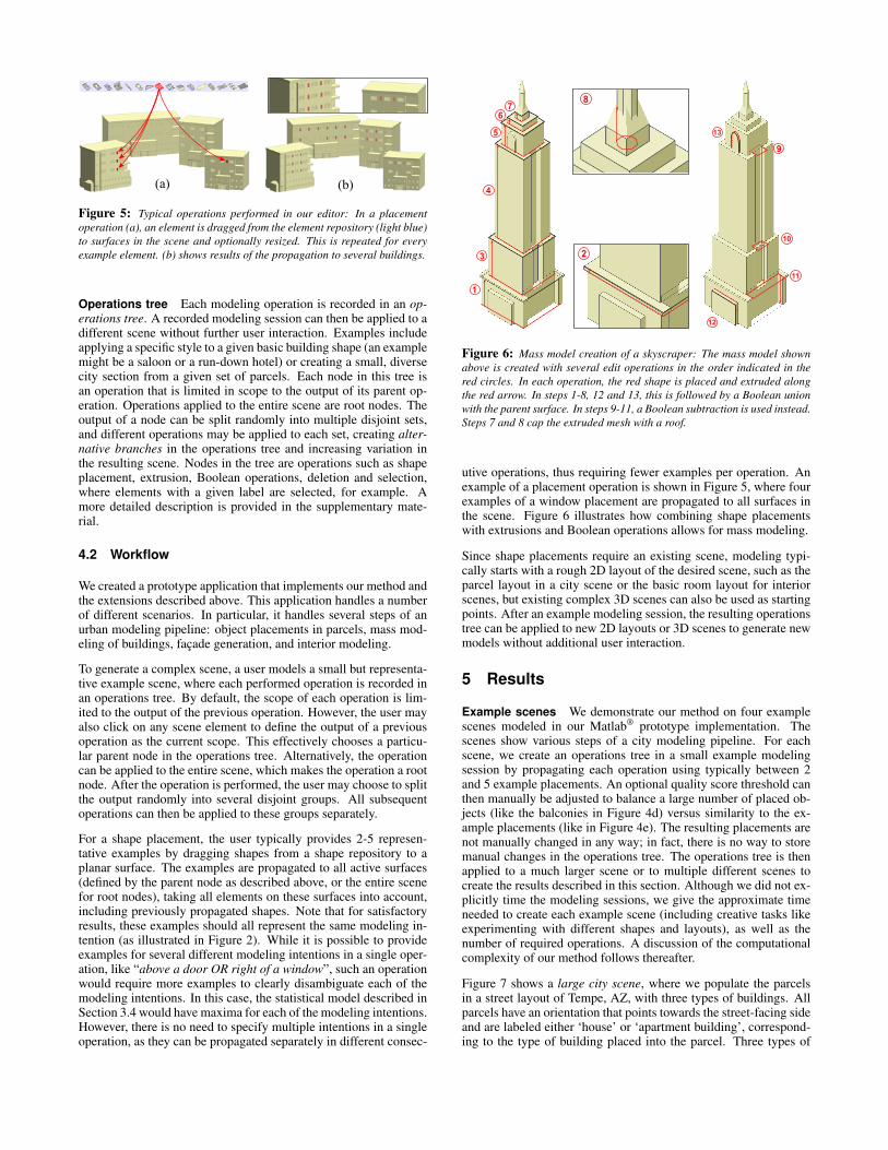
Figure 5: Typical operations performed in our editor: In a placementoperation (a), an element is dragged from the element repository (light blue)to surfaces in the scene and optionally resized. This is repeated for everyexample element. (b) shows results of the propagation to several buildings.

Operations tree Each modeling operation is recorded in an op-erations tree. A recorded modeling session can then be applied to adifferent scene without further user interaction. Examples includeapplying a specific style to a given basic building shape (an examplemight be a saloon or a run-down hotel) or creating a small, diversecity section from a given set of parcels. Each node in this tree isan operation that is limited in scope to the output of its parent op-eration. Operations applied to the entire scene are root nodes. Theoutput of a node can be split randomly into multiple disjoint sets,and different operations may be applied to each set, creating alter-native branches in the operations tree and increasing variation inthe resulting scene. Nodes in the tree are operations such as shapeplacement, extrusion, Boolean operations, deletion and selection,where elements with a given label are selected, for example. Amore detailed description is provided in the supplementary mate-rial.

4.2 Workflow

We created a prototype application that implements our method andthe extensions described above. This application handles a numberof different scenarios. In particular, it handles several steps of anurban modeling pipeline: object placements in parcels, mass mod-eling of buildings, facade generation, and interior modeling.

To generate a complex scene, a user models a small but representa-tive example scene, where each performed operation is recorded inan operations tree. By default, the scope of each operation is lim-ited to the output of the previous operation. However, the user mayalso click on any scene element to define the output of a previousoperation as the current scope. This effectively chooses a particu-lar parent node in the operations tree. Alternatively, the operationcan be applied to the entire scene, which makes the operation a rootnode. After the operation is performed, the user may choose to splitthe output randomly into several disjoint groups. All subsequentoperations can then be applied to these groups separately.

For a shape placement, the user typically provides 2-5 represen-tative examples by dragging shapes from a shape repository to aplanar surface. The examples are propagated to all active surfaces(defined by the parent node as described above, or the entire scenefor root nodes), taking all elements on these surfaces into account,including previously propagated shapes. Note that for satisfactoryresults, these examples should all represent the same modeling in-tention (as illustrated in Figure 2). While it is possible to provideexamples for several different modeling intentions in a single oper-ation, like “above a door OR right of a window”, such an operationwould require more examples to clearly disambiguate each of themodeling intentions. In this case, the statistical model described inSection 3.4 would have maxima for each of the modeling intentions.However, there is no need to specify multiple intentions in a singleoperation, as they can be propagated separately in different consec-

1

9

10

11

12

13

23

4

5

67

8

Figure 6: Mass model creation of a skyscraper: The mass model shownabove is created with several edit operations in the order indicated in thered circles. In each operation, the red shape is placed and extruded alongthe red arrow. In steps 1-8, 12 and 13, this is followed by a Boolean unionwith the parent surface. In steps 9-11, a Boolean subtraction is used instead.Steps 7 and 8 cap the extruded mesh with a roof.

utive operations, thus requiring fewer examples per operation. Anexample of a placement operation is shown in Figure 5, where fourexamples of a window placement are propagated to all surfaces inthe scene. Figure 6 illustrates how combining shape placementswith extrusions and Boolean operations allows for mass modeling.

Since shape placements require an existing scene, modeling typi-cally starts with a rough 2D layout of the desired scene, such as theparcel layout in a city scene or the basic room layout for interiorscenes, but existing complex 3D scenes can also be used as startingpoints. After an example modeling session, the resulting operationstree can be applied to new 2D layouts or 3D scenes to generate newmodels without additional user interaction.

5 Results

Example scenes We demonstrate our method on four examplescenes modeled in our Matlab® prototype implementation. Thescenes show various steps of a city modeling pipeline. For eachscene, we create an operations tree in a small example modelingsession by propagating each operation using typically between 2and 5 example placements. An optional quality score threshold canthen manually be adjusted to balance a large number of placed ob-jects (like the balconies in Figure 4d) versus similarity to the ex-ample placements (like in Figure 4e). The resulting placements arenot manually changed in any way; in fact, there is no way to storemanual changes in the operations tree. The operations tree is thenapplied to a much larger scene or to multiple different scenes tocreate the results described in this section. Although we did not ex-plicitly time the modeling sessions, we give the approximate timeneeded to create each example scene (including creative tasks likeexperimenting with different shapes and layouts), as well as thenumber of required operations. A discussion of the computationalcomplexity of our method follows thereafter.

Figure 7 shows a large city scene, where we populate the parcelsin a street layout of Tempe, AZ, with three types of buildings. Allparcels have an orientation that points towards the street-facing sideand are labeled either ‘house’ or ‘apartment building’, correspond-ing to the type of building placed into the parcel. Three types of

Figure 7: Given a set of labeled parcels, large city areas can be generated by our method without further user interaction. Three different types of houses(condominium building, two-story house and one-story house) were generated in three editing sessions. The resulting operations tree was applied to four citymaps shown in the inset on the left. The left image is taken from the lower-right tile, the right image from the upper-left tile.

houses are generated in the parcels: two types of family houses andone apartment building type. The example modeling session wasdone on a scene with 7 houses and 2–6 examples were providedfor each operation. Note how the building shape and consequentlythe facade details are determined by the parcel size, creating variedhouse models. Other sources of variation are the random selectionof alternative branches in the operations tree and the use of randomextrusion heights, as described in Section 4. The example modelingsession took approximately 3.5 hours: one hour for each of the twofamily houses and ~ 1.5 hours for the apartment building. A total of135 operations (including selections) were used to create all threebuilding types.

Figure 1 shows a scene with New York-style skyscrapers, wherewe apply an operations tree to coarse footprints of the skyscrapers.Nine skyscrapers were part of the example scene and between 2 and8 examples were provided in each operation. Variation is generatedin part through the skyscraper footprints and in part through ran-dom selection operations and extrusions with random height. Cre-ating the example scene took around 4 hours and was split into fourediting sessions: mass modeling (~ 1.5 hours), facades on the basefloors of the skyscrapers (~ 1.5 hours), on the center floors (~ 0.5hours) and on the top floors (~ 0.5 hours). All together, 146 opera-tions were performed in these four editing sessions.

Figure 8 shows a subset of various kitchen scenes that we gener-ated, where we applied an operations tree to single rooms. Thestarting point in this example is a polygon defining the shape of theroom and labels indicating walls with a planned door. The examplescene contained 9 kitchens and 2–6 examples were given in eachoperation. Note how the furniture adapts to the shape of each room,creating variation in the scenes. Additionally, alternative branchesin the tree were used to place different window styles and furni-ture models. In total, 85 operations were performed in a modelingsession that took around 3 hours.

Three Japanese garden scenes are shown in Figure 9. These were

generated from 2D layouts of paths, lakes, stone gardens and pavil-ion footprints. One of the gardens was used as the example scene(marked in the figure), which was created with 18 operations in ap-proximately one hour, with 2–6 examples given for each operation.Variation is generated mainly by adaption to the input layout, aswell as alternative branches in the operations tree for pavilions withor without roofs.

Computational complexity The computational complexity ofthe method mainly depends on the number of example placementsNe, the number of points Np in the position grid defined in Sec-tion 3.5, and the maximum number of elements Nf with the samelabel and type in the example feature sets. Since we use a kernelmethod, the feature sets of all grid points have to be compared tothe feature sets of all example placements. For each pair of featuresets, one assignment problem has to be solved with a maximumsize given by the number of elements with same type and label, asdefined in Equations (2) and (3). The resulting computational com-plexity is O(Ne ·Np ·N3

f ). In practice, Nf does not depend on thescene size, since increasing the scene complexity usually only in-creases the number of independent surfaces or hierarchy polygons,like facades or parcels, while the number of mutually dependentelements inside these areas stays more or less constant. Ne is usu-ally independent of the scene size as well; typically a user provides2-10 example placements. This leaves the term Np, which directlydepends on the scene size, giving our method a linear time complex-ity in practice. In practice, operations typically take between halfa second up to one minute. In the most demanding scenes, like theskyscraper facades with hundreds of elements on a single facade, apropagation can even take several minutes in our unoptimized Mat-lab prototype. These timings can certainly be improved in futurework. For example, the relations between each sample grid en-try and the surrounding geometry are computed directly in Matlab,taking every facade element into account. Considering only thoseelements that can actually have a significant contribution could al-ready provide a large speedup.

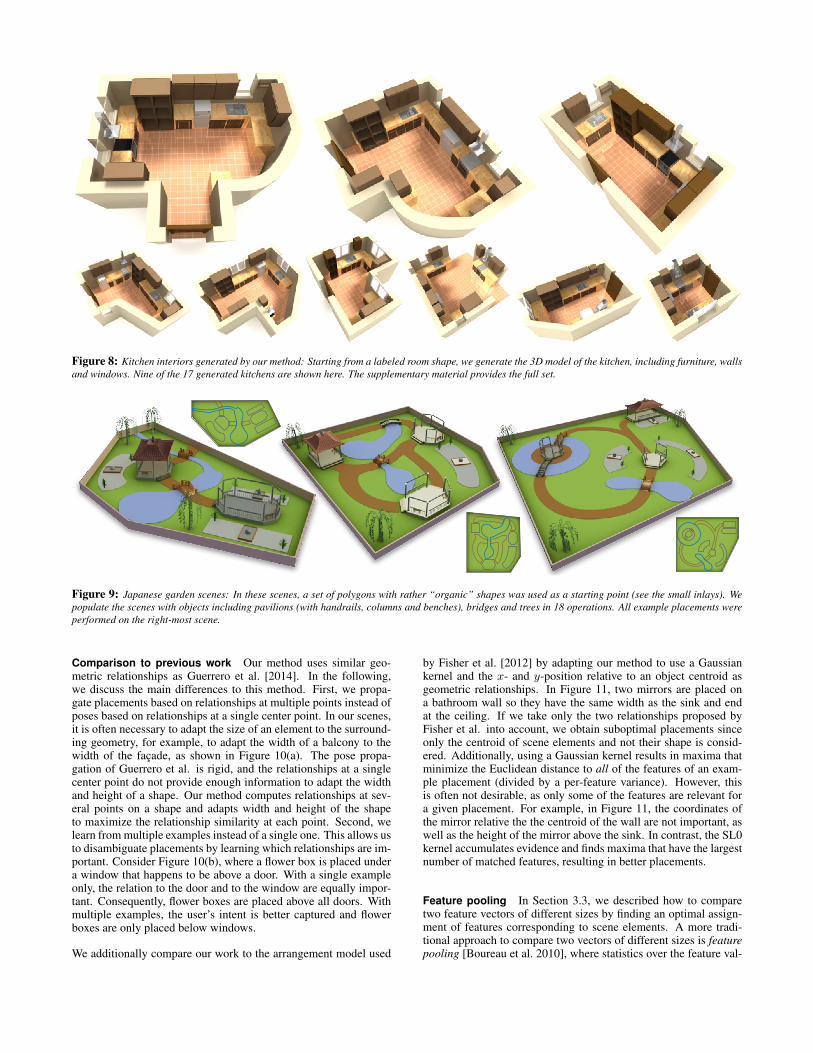
Figure 8: Kitchen interiors generated by our method: Starting from a labeled room shape, we generate the 3D model of the kitchen, including furniture, wallsand windows. Nine of the 17 generated kitchens are shown here. The supplementary material provides the full set.

Figure 9: Japanese garden scenes: In these scenes, a set of polygons with rather “organic” shapes was used as a starting point (see the small inlays). Wepopulate the scenes with objects including pavilions (with handrails, columns and benches), bridges and trees in 18 operations. All example placements wereperformed on the right-most scene.

Comparison to previous work Our method uses similar geo-metric relationships as Guerrero et al. [2014]. In the following,we discuss the main differences to this method. First, we propa-gate placements based on relationships at multiple points instead ofposes based on relationships at a single center point. In our scenes,it is often necessary to adapt the size of an element to the surround-ing geometry, for example, to adapt the width of a balcony to thewidth of the facade, as shown in Figure 10(a). The pose propa-gation of Guerrero et al. is rigid, and the relationships at a singlecenter point do not provide enough information to adapt the widthand height of a shape. Our method computes relationships at sev-eral points on a shape and adapts width and height of the shapeto maximize the relationship similarity at each point. Second, welearn from multiple examples instead of a single one. This allows usto disambiguate placements by learning which relationships are im-portant. Consider Figure 10(b), where a flower box is placed undera window that happens to be above a door. With a single exampleonly, the relation to the door and to the window are equally impor-tant. Consequently, flower boxes are placed above all doors. Withmultiple examples, the user’s intent is better captured and flowerboxes are only placed below windows.

We additionally compare our work to the arrangement model used

by Fisher et al. [2012] by adapting our method to use a Gaussiankernel and the x- and y-position relative to an object centroid asgeometric relationships. In Figure 11, two mirrors are placed ona bathroom wall so they have the same width as the sink and endat the ceiling. If we take only the two relationships proposed byFisher et al. into account, we obtain suboptimal placements sinceonly the centroid of scene elements and not their shape is consid-ered. Additionally, using a Gaussian kernel results in maxima thatminimize the Euclidean distance to all of the features of an exam-ple placement (divided by a per-feature variance). However, thisis often not desirable, as only some of the features are relevant fora given placement. For example, in Figure 11, the coordinates ofthe mirror relative the the centroid of the wall are not important, aswell as the height of the mirror above the sink. In contrast, the SL0kernel accumulates evidence and finds maxima that have the largestnumber of matched features, resulting in better placements.

Feature pooling In Section 3.3, we described how to comparetwo feature vectors of different sizes by finding an optimal assign-ment of features corresponding to scene elements. A more tradi-tional approach to compare two vectors of different sizes is featurepooling [Boureau et al. 2010], where statistics over the feature val-

A o

nly

pose

plac

emen

t

A,B

and

CAA B CA B C

exam

ples

exam

ples

(a) (b) (c)

Figure 10: Comparison of poses versus placements, as well as single ex-amples versus multiple examples: In (a), we show that using multiple instadof a single example point allows adaption of the shape to the surroundinggeometry (windows). In (b), the ambigous placement of the flower box inexample A (above a door or below a window) can be resolved when us-ing additional examples B and C. Providing multiple examples for doors onempty facades in (c) makes it clear that doors should maintain their size(bottom row) instead of adapting to the size of the facade (center row).

example 1 example 2 Fisher rel., Gaussian kernel our rel., Gaussian kernel

Fisher rel., SL0 kernel our rel., SL0 kernel

Figure 11: Comparison to Fisher et al. [2012] for propagating the twomirror placements shown on the left. We show the propagated mirrors (red)and the prediction for the top left corner of the mirror as heat maps inthe background for the two relationships proposed by Fisher et al. (centercolumn) versus our relationships (right column) and for a Gaussian kernel(top row) versus the SL0 kernel (bottom row). Our method (bottom right)finds the best interpretation of example placements: ‘Same width as the sinkand ending at the ceiling.’

ues are extracted. Figure 12 compares two feature-pooling methodsto our approach. If we use only the relationships to the three closestelements, the implied assignment fails to correctly identify the rele-vant elements and results in bad placements, indicated by the num-bered windows. Similarly, histograms are not usable since they alsoinclude the contributions of irrelevant elements (i.e., the windowson the first floor). Our approach finds the assignment that maxi-mizes the similarity to the examples and thereby correctly identifiesthe relevant elements.

Deformation tolerance and overlap filter Although the focusof this paper is learning the relationships of shapes to surroundingscene elements, but not the properties of the shapes themselves, weprovided a simple way to optionally penalize shape deformation inSection 3.5. The effect of the deformation tolerance is illustrated inFigure 13(a). Similarly, we focus on placing single shapes but noshape arrangements. In Section 3.5, we also provided a simple wayto avoid overlap between those candidate placements presented tothe user. Figure 13(b) shows the effects of this filter on a scene withthree potentially good placements of the example balcony. Withoutthe filter, all three placements are presented to the user. In contrast,the overlapping placements with a lower score are removed by thefilter.

window distance0 maxwindow distance0 max

1 1

2

31 2 3 2 3

example (a) 3 closest elements (b) histograms (c) assignment

Figure 12: Comparison to feature pooling: The balcony on the left ispropagated using the three closest scene elements only (a), a histogram overfeature values (b) and our scene element assignment (c). For the red point(correct position of the lower-left balcony corner), the implied assignmentbetween windows is indicated by the numbers in (a) and (c) and the his-togram of window distance values is shown in (b). Our approach comparesthe correct feature pairs and finds a good balcony placement (c).

example placements (a) distortion tol. (b) overlap filteroff on0.5∞

Figure 13: Effect of deformation tolerance and the overlap filter: Two ex-amples of a balcony placement on the left are propagated to the two scenesin (a) and (b). In (a), the distortion tolerance is set to infinity, i.e., turned off(left), and to a moderate value of 0.5 (right), while in (b), the overlap filter isturned off (left) and on (right). Depending on the situation, the resulting listof candidates (red) may be more useful when applying one of these filters.

Quantitative evaluation In Figure 14, we show detailed quanti-tative evaluations of our method and compare to previous work andthe variations of our own method as described above. A groundtruth was manually created for several shape placement operationsin the scenes shown on the left (only parts are shown here; the com-plete scenes are provided as supplementary material). Exhaustivecross validation (or repeated random sub-sampling cross validationwith a minimum of 25 splits if exhaustive cross-validation was notfeasible) was conducted to compare the results of each operationto the ground truth. The tested training set size was varied fromone to the number of ground truth placements. To simulate the useradjusting the score threshold for candidate placements, we chosethe optimal threshold with respect to the ground truth in each op-eration (in all of the tested methods). The average F1-score (i.e.,the harmonic mean of precision and recall) of our method over alloperations compared to previous methods is shown in the center ofFigure 14. These evaluations support our conclusion that learningfrom multiple examples significantly increases the quality of prop-agated placements. In the table on the right, we show the averageF1-score over typical sets of 2-5 examples. The proposed methodresults in placements with significantly higher quality than the gen-erated by existing methods. Since Guerrero et al. [2014] only usea single example and additionally cannot adapt the shape size, theupper bound for this method is given by the “single example” col-umn of the table. Using feature pooling with the closest three ele-ments is on average not much worse compared with our assignmentapproach. However, note that there are several scenes where thisapproach clearly provides sub-optimal results (e.g., the balconiesand windows in scene 1, decorations A and B in scene 2, classroomchairs in scene 3 in Figure 14), for the reasons discussed earlier.

Relationship influence The influence of each relationship typeon the score of a point is determined by the kernel. We show themost important relationships learned from two sample points of twoexample placements in Figure 15. Note that the wall light varies insize, but like the example placements, the mirror remains at the sizeof the sink. The effect of learning the examples is noticeable in the

scen

e 1

scen

e 2

scen

e 3

scen

e 4

0.2

0.6

1

0.2

0.2

0.6

0.6

1

1

0.4

0.7

1

1 4 8 12 16

F1 score

# examples

93 5 71

2 3 4 5 61

2 3 4 5 61

# placem

ents

Fisher

Gaussi

an

allGau

ssian

Fisher

SL0

histog

rampo

oling

closes

t 3po

oling

single

exam

ple

ours o

verlapfilter)

ours

. filter)

ours

doors 16 0.62 0.73 0.54 0.87 0.89 0.70 0.84 0.90 0.89flowerboxes 14 0.14 0.17 0.69 0.46 0.67 0.48 0.82 0.67 0.75

balconies 24 0.03 0.02 0.65 0.36 0.74 0.59 0.84 0.84 0.89doorsigns 16 0.17 0.33 0.65 0.80 0.96 0.78 0.96 0.96 0.96

windowframes 133 0.00 0.00 0.80 0.25 0.97 0.93 0.94 0.81 0.97door roofs 15 0.20 0.24 0.74 0.68 0.86 0.59 0.90 0.85 0.87

windows 18 0.03 0.03 0.72 0.37 0.59 0.47 0.78 0.73 0.71scene1 average 0.17 0.22 0.68 0.54 0.81 0.65 0.87 0.82 0.86

edit operation

F1 scores

F1 scores

F1 scores

F1 scores

windows 8 0.29 0.39 0.26 0.80 0.85 0.58 0.70 0.75 0.82columns 9 0.38 0.37 0.55 0.58 0.71 0.55 0.73 0.68 0.73staircase 13 0.21 0.31 0.50 0.47 0.72 0.57 0.73 0.59 0.70

balconies 19 0.04 0.03 0.45 0.49 0.76 0.53 0.71 0.68 0.77decorations A 32 0.00 0.00 0.80 0.31 0.72 0.60 0.82 0.73 0.88

door frames 12 0.25 0.21 0.95 0.70 0.95 0.89 0.97 0.94 0.96decorations B 10 0.00 0.00 0.95 0.27 0.76 0.60 0.96 0.95 0.95

scene 2 average 0.17 0.19 0.64 0.52 0.78 0.62 0.80 0.76 0.83

beds 6 0.29 0.29 0.94 0.60 0.95 0.78 0.92 0.95 0.94night tables 7 0.62 0.62 0.82 0.70 0.81 0.74 0.90 0.85 0.82

rugs 6 0.01 0.01 0.69 0.34 0.69 0.46 0.73 0.63 0.69desk chairs 12 0.11 0.11 0.75 0.44 0.75 0.37 0.77 0.79 0.75

classroom chairs 7 0.00 0.00 0.83 0.01 0.21 0.34 0.86 0.83 0.83scene 3 average 0.21 0.21 0.81 0.42 0.68 0.54 0.84 0.81 0.81

pavilionbeams 34 0.07 0.07 0.93 0.63 0.90 0.83 0.94 0.56 0.93stone area 6 0.50 0.50 0.81 0.67 0.78 0.55 0.82 0.63 0.81

stones 5 0.71 0.71 0.74 0.75 0.79 0.71 0.82 0.69 0.82bridges 6 0.00 0.00 0.82 0.07 0.81 0.58 0.89 0.78 0.82

scene 4 average 0.32 0.32 0.82 0.53 0.82 0.67 0.87 0.66 0.84

(no defo

rm

(

Figure 14: Quantitative evaluation of several shape placement operations by cross-validating against a manually generated ground truth and comparisonwith the results of previous methods. In the center, the average F1-score over all edit operations is plotted as the number of examples selected from the groundtruth increases. Each curve corresponds to the method with the same line style in the table. The table shows the average F1-score for each edit operation overtypical sets of 2-5 examples. Part of the scenes are shown on the left. See the supplementary material for the complete scenes.

τ = 1 τ = 0.1 τ = 10examples

Figure 16: Effects of changing the kernel size: In two examples, a smallroof is placed between a door and a window (left). The score for the lowerleft edge point is shown as heat maps. The upper window is strongly mis-aligned, the lower window only slighty. With a small τ as the kernel size,both misalignments are too strong to be considered similar to the examples,while with a big kernel size, both misalignments are considered similar.

low weight of the normalized bounding box width relationship tothe lamp (second column, top row), compared to the same relation-ship in the bottom row.

Kernel size The size of the SL0 kernel is determined by the vari-ance of the Gaussians in the SL0 similarity. Each relationship typedefines a variance based on its range of values, e.g., a directionalrelationship requires a different variance than a relationship thatcomputes an absolute distance. Relationships based on an abso-lute distance use the bounding box diagonal of the placed shape tonormalize the variance. We can additionally multiply the varianceswith a constant factor τ to control the precision of the placements.Figure 16 shows the effect of changing τ . Lower values increasethe precision and decrease the tolerance, while higher values do theopposite. A good value of τ is a tradeoff between precision andtolerance. We use τ = 1 in all shown examples.

exam

ple

faca

des

gene

rate

dfa

cade

s

Figure 17: Results of applying an operations tree learned from unrepre-sentative examples: The operations tree for a family house was learned onsingle-story buildings (top row). When applied to two-story buildings, thereis ambiguity that results in unexpected element placements (bottom row).Providing addtional examples on two-story buildings would help to resolvethe ambiguity.

5.1 Limitations and Future Work

When an operations tree is created and example placements arelearned, the example scenes should represent the types of scenes theoperations tree is intended for. To illustrate this point, in Figure 17,an operations tree was generated from single-story buildings only.By applying this operations tree to buildings with two stories, toomuch unresolved ambiguity remains. For example, should the en-trance be placed on the first or second floor, or should it cover bothfloors? Since our method mostly operates on a geometric level,

boundary distancenorm. boundgboxboundingbox x yy

B to

lam

pA

to si

nk

norm. boundingbox combined

A A

B

B

Figure 15: Learned importance of individual relationships: A mirror placement between a sink of fixed size and a wall light of varying width is learned fromtwo examples. Scores of individual relationships are shown as heat map on the right. For more information on the relationship types, see Appendix A.2.

these questions could be resolved by providing additional exam-ples.

In future work, we would like to extend our method to include ge-ometric relationships in the full 3D space. This would allow plac-ing 3D shapes anywhere in the scene, not only on planar surfacesof objects. Also, we currently propagate point placements withoutconsidering their orientation relative to the surrounding scene el-ements. Guerrero et al. [2014] show that this relative orientationcan be described by several interesting geometric relationships thatwould enrich our statistical model. Finally, extending our definitionof placements to include more general deformations would allow abetter adaption of the propagated shapes to the surrounding geom-etry, but would also require a new technique to find the maxima ofour statistical model in the higher-dimensional space of placements.

6 Conclusion

We presented a method for placing shapes “by example” in 2Dscenes. In contrast to previous example-based placement methods,which are limited to a single example and a single representativepoint, our method learns a model from multiple example place-ments and takes the width, height and orientation of the examplesinto account. This is made possible by using kernel regression tolearn the user’s intent, with a kernel defined on a similarity metricthat can deal with heterogeneous feature sets. Quantitative evalu-ations show that learning from multiple examples significantly im-proves the quality of propagated placements.

We further generalize the 2D placement operation to 3D scenes us-ing extrusion and Boolean operations, which makes it possible toapply the method for a wide range of modeling tasks. Through anoperations tree that records operations carried out by the user, mod-eling sessions can be applied to different scenes. As an example,we have demonstrated how several steps in a city modeling pipelinecan be carried out efficiently using our application prototype.

Acknowledgements

We would like to thank Khaled Abd El Gawad and YoshihiroKobayashi for rendering the scenes shown in Section 5, as well asVirginia Unkefer for proof-reading the paper.

This publication is based upon work supported by the KAUSTOffice of Competitive Research Funds (OCRF) under Award No.62140401, the KAUST Visual Computing Center and the AustrianScience Fund (FWF) projects DEEP PICTURES (no. P24352-N23)and Data-Driven Procedural Modeling of Interiors (no. P24600-N23).

References

BISHOP, C. M. 2006. Pattern Recognition and Machine Learning(Information Science and Statistics). Springer-Verlag New York,Inc., Secaucus, NJ, USA.

BOKELOH, M., WAND, M., SEIDEL, H.-P., AND KOLTUN, V.2012. An algebraic model for parameterized shape editing. ACMTrans. Graph. 31, 4 (July), 78:1–78:10.

BOUREAU, Y.-L., PONCE, J., AND LECUN, Y. 2010. A theo-retical analysis of feature pooling in visual recognition. In 27thInternational Conference on Machine Learning, Haifa, Israel.

CHAUDHURI, S., KALOGERAKIS, E., GUIBAS, L., ANDKOLTUN, V. 2011. Probabilistic reasoning for assembly-based3d modeling. ACM Trans. Graph. 30, 4 (July), 35:1–35:10.

CUI, Z., ZHANG, H., AND LU, W. 2010. An improved smoothedl0-norm algorithm based on multiparameter approximation func-tion. In Communication Technology (ICCT), 2010 12th IEEEInternational Conference on, 942–945.

FISHER, M., AND HANRAHAN, P. 2010. Context-based search for3d models. ACM Trans. Graph. 29, 6 (Dec.), 182:1–182:10.

FISHER, M., SAVVA, M., AND HANRAHAN, P. 2011. Character-izing structural relationships in scenes using graph kernels. ACMTrans. Graph. 30, 4 (July), 34:1–34:12.

FISHER, M., RITCHIE, D., SAVVA, M., FUNKHOUSER, T., ANDHANRAHAN, P. 2012. Example-based synthesis of 3d objectarrangements. ACM Trans. Graph. 31, 6 (Nov.), 135:1–135:11.

FUNKHOUSER, T., KAZHDAN, M., SHILANE, P., MIN, P.,KIEFER, W., TAL, A., RUSINKIEWICZ, S., AND DOBKIN, D.2004. Modeling by example. ACM Trans. Graph. 23, 3, 652–663.

GAL, R., SORKINE, O., MITRA, N. J., AND COHEN-OR, D.2009. iWIRES: an analyze-and-edit approach to shape manip-ulation. ACM Trans. Graph. 28, 3 (July), 33:1–33:10.

GUERRERO, P., JESCHKE, S., WIMMER, M., AND WONKA, P.2014. Edit propagation using geometric relationship functions.ACM Trans. Graph. 33, 2 (Apr.), 15:1–15:15.

KALOGERAKIS, E., CHAUDHURI, S., KOLLER, D., ANDKOLTUN, V. 2012. A probabilistic model for component-basedshape synthesis. ACM Trans. Graph. 31, 4 (July), 55:1–55:11.

KITCHEN, L., AND ROSENFELD, A. 1982. Gray-level cornerdetection. Pattern Recognition Letters 1, 2, 95 – 102.

KUHN, H. W. 1955. The hungarian method for the assignmentproblem. Naval Research Logistics Quarterly 2, 1-2, 83–97.

MERRELL, P., SCHKUFZA, E., LI, Z., AGRAWALA, M., ANDKOLTUN, V. 2011. Interactive furniture layout using interiordesign guidelines. ACM Trans. Graph. 30, 4 (July), 87:1–87:10.

OXVIG, C. S., PEDERSEN, P. S., ARILDSEN, T., AND LARSEN,T. 2012. Improving smoothed l0 norm in compressive sensingusing adaptive parameter selection. CoRR abs/1210.4277.

XU, K., STEWART, J., AND FIUME, E. 2002. Constraint-BasedAutomatic Placement for Scene Composition. In Graphics In-terface, 25–34.

YEH, Y.-T., YANG, L., WATSON, M., GOODMAN, N. D., ANDHANRAHAN, P. 2012. Synthesizing open worlds with con-straints using locally annealed reversible jump mcmc. ACM TOG31, 4 (July), 56:1–56:11.

YU, L.-F., YEUNG, S.-K., TANG, C.-K., TERZOPOULOS, D.,CHAN, T. F., AND OSHER, S. J. 2011. Make it home: automaticoptimization of furniture arrangement. ACM Trans. Graph. 30,4 (July), 86:1–86:12.

ZHENG, Y., FU, H., COHEN-OR, D., AU, O. K.-C., ANDTAI, C.-L. 2011. Component-wise controllers for structure-preserving shape manipulation. Computer Graphics Forum 30,2, 563–572.

A Scene Elements and Relationship Func-tions

A.1 Scene Elements

Relationship functions use the following scene elements:

• a polygon A, defined by a sequence of vertices vk, wherek ∈ {1, . . . , nA},

• a polygon segment gj ⊆ A, defined as a subsequence ofconsecutive smooth vertices gj = va, . . . ,vb, where a, b ∈{1, . . . , nA}. A vertex is called smooth if the dot prod-uct of its adjacent edges is above a threshold ( vk+1−vk

||vk+1−vk||·

vk−vk−1

||vk−vk−1||> ε), otherwise it is called sharp,

• a corner cj of a polygon, defined by a vertex vkj that isshared by two adjacent segments gj−1 and gj . Corners corre-spond to sharp vertices.

A.2 Relationship Functions

We use three relationship functions, one for each element type.These functions compute tuples of geometric relationships. Forpolygon elements, we compute a 3-tuple, consisting of three val-ues:

• The boundary distance is defined as the minimum distancebetween a point and a polygon boundary: Rbd(p, A) =minx∈b(A) d(p,x), where b(A) is the boundary of A and dthe Euclidean distance.

• The bounding box coordinates are defined as the x and y-components of the cartesian coordinates in the local coordi-nate frame of a polygon with origin at the bounding box mini-mum, the bounding box maximum and the bounding box cen-ter of the polygon, for a total of six relationship functions.

• The normalized bounding box coordinates are boundingbox coordinates with origin at the bounding box minimum,normalized to the width and height of the bounding box.

For segment elements, we compute a 2-tuple:

• The segment distance Rgd(p, g) is the same as the boundarydistance, but considers only a segment g ∈ A.

• The segment arc length is the normalized arc length betweenthe location of minimum distance to a point p and the startof the segment. If x = arg minx∈b(gj) d(p,x), then Rgl =tx−tatb−ta

, where tx is the arc length at x and ta, tb the arc lengthat the start and the end of the segment, respectively.

For corner elements, we compute a 2-tuple:

• The corner distance is the distance between a point and apolygon corner: Rcd(p, cj) = d(p,vkj ).

• The corner ratio is the angle that the direction fromcorner to point p makes with the start of the firstpolygon segment adjacent to the corner, normalizedwith the opening angle of the corner: Rcr(p, cj) =

∠(p−vkj,vkj−1−vkj

)

∠(vkj+1−vkj,vkj−1−vkj

), where ∠(a,b) is the angle be-

tween vectors: ∠(a,b) = arccos(

a||a|| ·

b||b||

).