Learning to Encode Position for Transformerwith Continuous Dynamical Model

Xuanqing Liu†, Hsiang-Fu Yu‡, Inderjit Dhillon§‡, Cho-Jui Hsieh†

† UCLA § UT Austin ‡ Amazon Inc.

xqliu@cs.ucla.edu rofu.yu@gmail.com

inderjit@cs.utexas.edu chohsieh@cs.ucla.edu

Abstract

We introduce a new way of learning to encode position information for non-recurrent models,such as Transformer models. Unlike RNN and LSTM, which contain inductive bias by loadingthe input tokens sequentially, non-recurrent models are less sensitive to position. The main reasonis that position information among input units is not inherently encoded, i.e., the models arepermutation equivalent; this problem justifies why all of the existing models are accompanied bya sinusoidal encoding/embedding layer at the input. However, this solution has clear limitations:the sinusoidal encoding is not flexible enough as it is manually designed and does not containany learnable parameters, whereas the position embedding restricts the maximum length of inputsequences. It is thus desirable to design a new position layer that contains learnable parameters toadjust to different datasets and different architectures. At the same time, we would also like theencodings to extrapolate in accordance with the variable length of inputs. In our proposed solution,we borrow from the recent Neural ODE approach, which may be viewed as a versatile continuousversion of a ResNet. This model is capable of modeling many kinds of dynamical systems. Wemodel the evolution of encoded results along position index by such a dynamical system, therebyovercoming the above limitations of existing methods. We evaluate our new position layers on avariety of neural machine translation and language understanding tasks, the experimental resultsshow consistent improvements over the baselines.

1 Introduction

Transformer based models [1, 2, 3, 4, 5, 6] have become one of the most effective approaches tomodel sequence data of variable lengths. Transformers have shown wide applicability to many naturallanguage processing (NLP) tasks such as language modeling [4], neural machine translation (NMT) [1],and language understanding [2]. Unlike traditional recurrent-based models (e.g., RNN or LSTM),Transformer utilizes a non-recurrent but self-attentive neural architecture to model the dependencyamong elements at different positions in the sequence, which leads to better parallelization usingmodern hardware and alleviates the vanishing/exploding gradient problem in traditional recurrentmodels.[7] prove that the design of self-attentive architecture leads to a family of permutation equivalencefunctions. Thus, for applications where the ordering of the elements matters, how to properly encodeposition information is crucial for Transformer based models. There have been many attempts toencode position information for the Transformer. In the original Transformer paper [1], a family of

1

arX

iv:2

003.

0922

9v1

[cs

.LG

] 1

3 M

ar 2

020

pre-defined sinusoidal functions was adapted to construct a set of embeddings for each position. Thesefixed position embeddings are then added to the word embeddings of the input sequence accordingly.To further construct these position embeddings in a more data-driven way, many recent Transformervariants such as [2, 8] include these embeddings as learnable model parameters in the training stage.This data-driven approach comes at the cost of the limitation of a fixed maximum length of inputsequence Lmax and the computational/memory overhead of additional Lmax × d parameters, whereLmax is usually set to 512 in many applications, and d is the dimension of the embeddings. [9] proposea relative position representation to reduce the number of parameters to (2K + 1)d by dropping theinteractions between tokens with a distance greater than K. In addition to just the input layer, [10] and[5] suggest that the injection of position information to every layer leads to even better performance forthe Transformer.An ideal position encoding approach should satisfy the following three properties:1. Inductive: the ability to handle sequences longer than any sequence seen in the training time.2. Data-Driven: the position encoding should be learnable from the data.3. Parameter Efficient: number of trainable parameters introduced by the encoding should be limited

to avoid increased model size, which could hurt generalization.In Table 1, we summarize some of the existing position encoding approaches in terms of these threeproperties.In this paper, we propose a new method to encode position with minimum cost. The main idea isto model position encoding as a continuous dynamical system, so we only need to learn the systemdynamics instead of learning the embeddings for each position independently. By doing so, ourmethod enjoys the best of both worlds – we bring back the inductive bias, and the encoding methodis freely trainable while being parameter efficient. To enable training of this dynamical system withbackpropagation, we adopt the recent progress in continuous neural network [11], officially calledNeural ODE. In some generative modeling literature, it is also called the free-form flow model [12],so we call our model FLOw-bAsed TransformER (FLOATER). We highlight our contributions asfollows:• We propose FLOATER, a new position encoder for Transformer, which models the position informa-

tion via a continuous dynamical model in a data-driven and parameter-efficient manner.• Due to the use of a continuous dynamic model, FLOATER can handle sequences of any length. This

property makes inference more flexible.• With careful design, our position encoder is compatible with the original Transformer; i.e., the

original Transformer can be regarded as a special case of our proposed position encoding approach.As a result, we are not only able to train a Transformer model with FLOATER from scratch but alsoplug FLOATER into most existing pre-trained Transformer models such as BERT, RoBERTa, etc.• We demonstrate that FLOATER consistent improvements over baseline models across a variety of

NLP tasks ranging from machine translations, language understanding, and question answering.

2 Background and Related Work

2.1 Importance of Position Encoding for Transformer

We use a simplified self-attentive sequence encoder to illustrate the importance of position encoding inthe Transformer. Without position encoding, the Transformer architecture can be viewed as a stack ofN blocks Bn : n = 1, . . . , N containing a self-attentive An and a feed-forward layer Fn. By droppingthe residual connections and layer normalization, the architecture of a simplified Transformer encoder

2

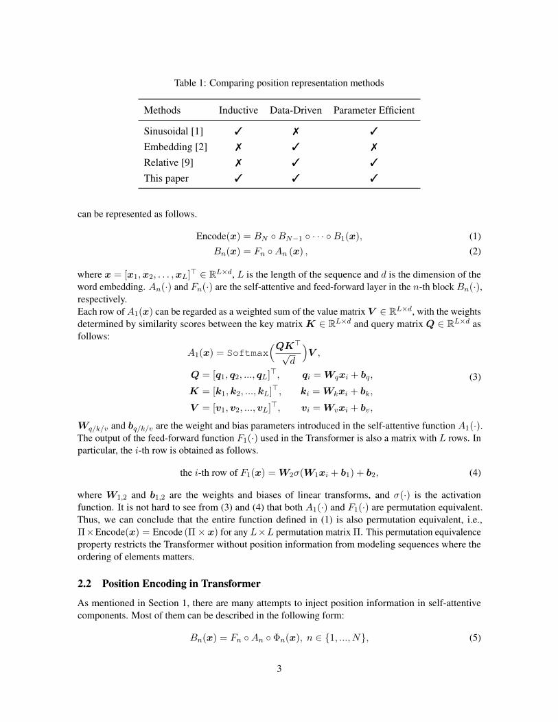
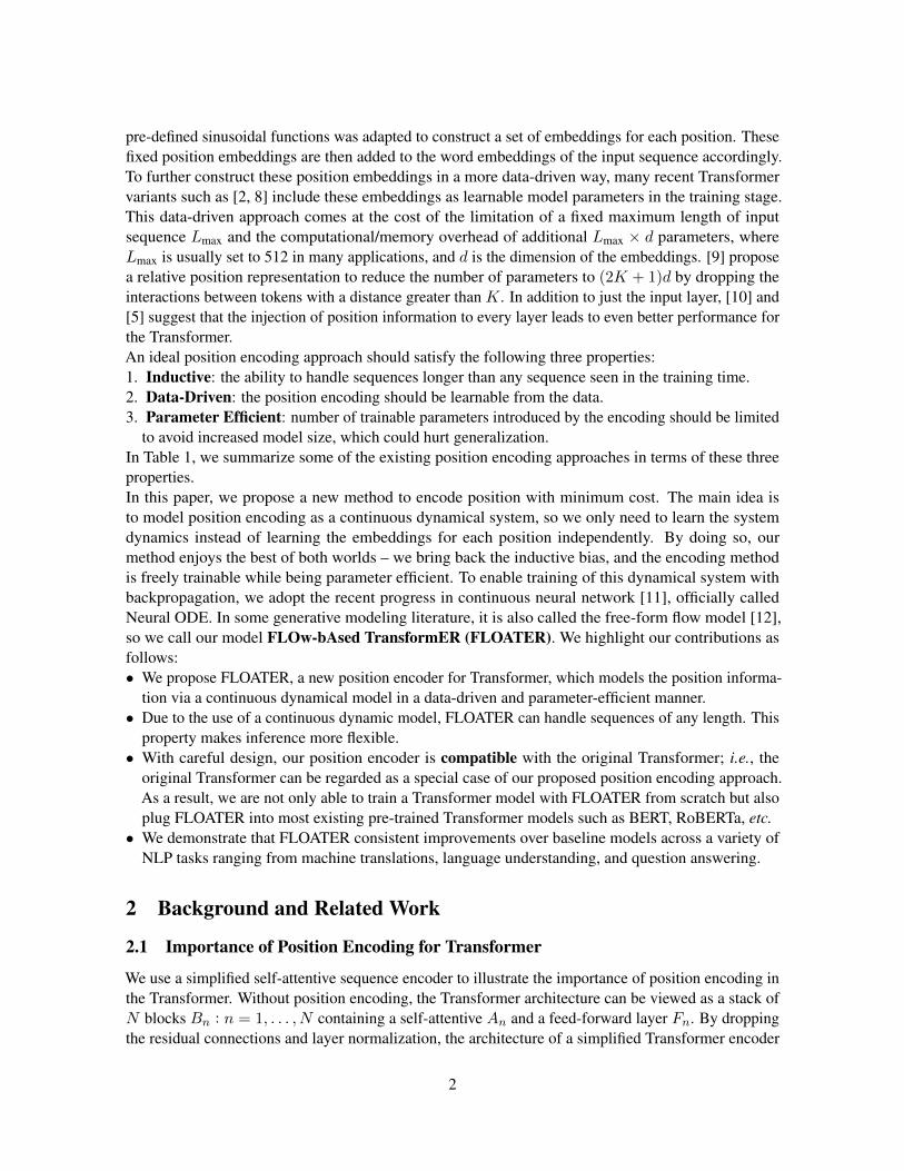
Table 1: Comparing position representation methods

Methods Inductive Data-Driven Parameter Efficient

Sinusoidal [1] 3 7 3

Embedding [2] 7 3 7

Relative [9] 7 3 3

This paper 3 3 3

can be represented as follows.

Encode(x) = BN ◦BN−1 ◦ · · · ◦B1(x), (1)

Bn(x) = Fn ◦An (x) , (2)

where x = [x1,x2, . . . ,xL]> ∈ RL×d, L is the length of the sequence and d is the dimension of theword embedding. An(·) and Fn(·) are the self-attentive and feed-forward layer in the n-th block Bn(·),respectively.Each row of A1(x) can be regarded as a weighted sum of the value matrix V ∈ RL×d, with the weightsdetermined by similarity scores between the key matrix K ∈ RL×d and query matrix Q ∈ RL×d asfollows:

A1(x) = Softmax(QK>√

d

)V ,

Q = [q1, q2, ..., qL]>, qi = Wqxi + bq,

K = [k1,k2, ...,kL]>, ki = Wkxi + bk,

V = [v1,v2, ...,vL]>, vi = Wvxi + bv,

(3)

Wq/k/v and bq/k/v are the weight and bias parameters introduced in the self-attentive function A1(·).The output of the feed-forward function F1(·) used in the Transformer is also a matrix with L rows. Inparticular, the i-th row is obtained as follows.

the i-th row of F1(x) = W2σ(W1xi + b1) + b2, (4)

where W1,2 and b1,2 are the weights and biases of linear transforms, and σ(·) is the activationfunction. It is not hard to see from (3) and (4) that both A1(·) and F1(·) are permutation equivalent.Thus, we can conclude that the entire function defined in (1) is also permutation equivalent, i.e.,Π×Encode(x) = Encode (Π× x) for any L×L permutation matrix Π. This permutation equivalenceproperty restricts the Transformer without position information from modeling sequences where theordering of elements matters.

2.2 Position Encoding in Transformer

As mentioned in Section 1, there are many attempts to inject position information in self-attentivecomponents. Most of them can be described in the following form:

Bn(x) = Fn ◦An ◦ Φn(x), n ∈ {1, ..., N}, (5)

3

Self-Attention

FFN

Add & norm

Add & norm

Position encodingat the k-th layer

Hidden feature

Flow-based transition model

L×

FLOATER-Encoder

Self-Attention

FFN

Add & norm

Position encodingat the k-th layer

Hidden feature

Flow-based transition model

L×

FLOATER-Decoder

Add & norm

Enc-Dec-Attention

Add & norm

Figure 1: The architecture of our model (FLOATER). The main differences between FLOATER andthe original Transformer model are: 1) the position representation is integrated into each block inthe hierarchy (there are N blocks in total); and 2) there is a dynamical model (see (8)) that generatesposition encoding vectors for each block. The dynamics are solved with a black-box ODE solverdetailed in the supplementary material.

where Φn(x) is a position encoding function.[1] propose to keep Φn(x) = x, ∀n ≥ 2 and inject position information only at the input block with afamily of pre-defined sinusoidal functions: Φ1(x) = x+ p(1), where p(1) = [p

(1)1 ,p

(1)2 , ...,p

(1)L ] is a

position embedding matrix with the i-th row corresponding to the i-th position in the input sequence.In particular, the j-th dimension of the i-th row is defined as follows.

p(1)i [j] =

sin(i · c jd ) if j is even,

cos(i · c j−1d ) if j is odd,

(6)

where c = 10−4. [10] and [5] observe better performance by further injecting the position informationat each block, i.e., Φn(x) = x+ p(n) as follows:

p(n)i [j] =

sin(i · c jd ) + sin(n · c j

d ) if j is even,

cos(i · c j−1d ) + cos(n · c j−1

d ) if j is odd.(7)

Note that for the above two approaches, position encoding functions Φn(·) are fixed for all theapplications. Although no additional parameters are introduced in the model, both approaches areinductive and can handle input sequences of variable length.Many successful variants of pre-trained Transformer models, such as BERT [2] and RoBERTa [8],include the entire embedding matrix p(1) ∈ RL×d in Φ1(x) as training parameters. As the numberof training parameters needs to be fixed, the maximum length of a sequence, Lmax, is required to bedetermined before the training. Although it lacks the inductive property, this data-driven approach isfound to be effective for many NLP tasks. Note that, unlike the fixed sinusoidal position encoding,there is no attempt to inject a learnable position embedding matrix at each block for Transformer dueto a large number of additional parameters (NLmaxd).

4

3 FLOATER: Our Proposed Position Encoder

We introduce our method in three steps. In the first step, we only look at one Transformer block, anddescribe how to learn the position representation driven by a dynamical system; in the second step, weshow how to save parameters if we add position signals to every layer; lastly, we slightly change thearchitecture to save trainable parameters further and make FLOATER “compatible” with the originalTransformer [1]. The compatibility means our model is a strict superset of the vanilla Transformer sothat it can be initialized from the Transformer.

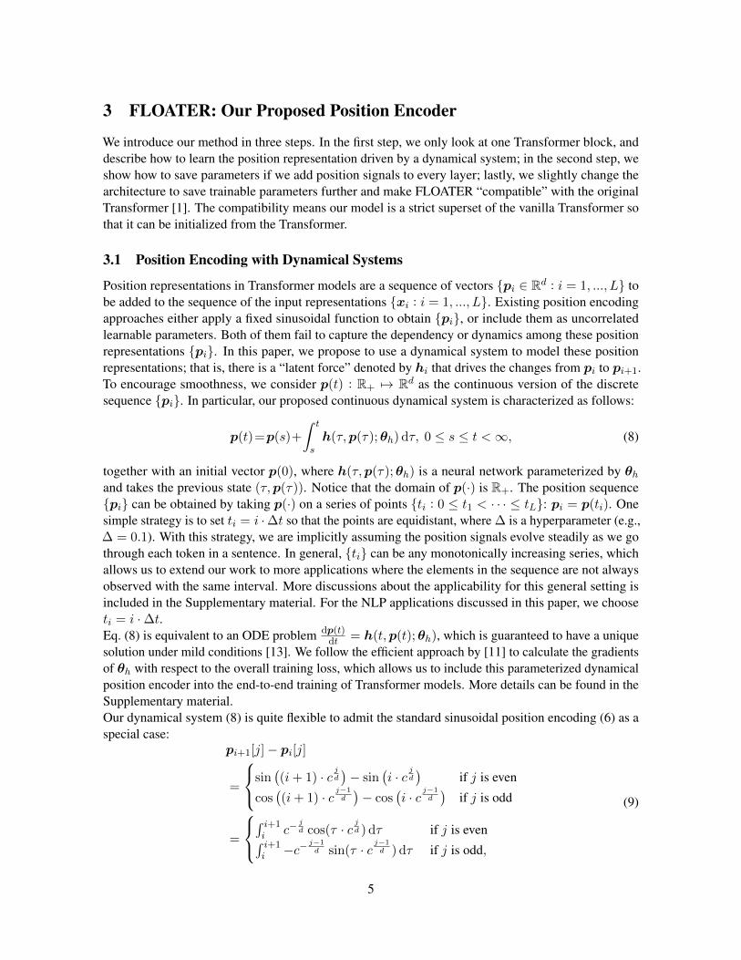
3.1 Position Encoding with Dynamical Systems

Position representations in Transformer models are a sequence of vectors {pi ∈ Rd : i = 1, ..., L} tobe added to the sequence of the input representations {xi : i = 1, ..., L}. Existing position encodingapproaches either apply a fixed sinusoidal function to obtain {pi}, or include them as uncorrelatedlearnable parameters. Both of them fail to capture the dependency or dynamics among these positionrepresentations {pi}. In this paper, we propose to use a dynamical system to model these positionrepresentations; that is, there is a “latent force” denoted by hi that drives the changes from pi to pi+1.To encourage smoothness, we consider p(t) : R+ 7→ Rd as the continuous version of the discretesequence {pi}. In particular, our proposed continuous dynamical system is characterized as follows:

p(t)=p(s)+

∫ t

sh(τ,p(τ);θh) dτ, 0 ≤ s ≤ t <∞, (8)

together with an initial vector p(0), where h(τ,p(τ);θh) is a neural network parameterized by θhand takes the previous state (τ,p(τ)). Notice that the domain of p(·) is R+. The position sequence{pi} can be obtained by taking p(·) on a series of points {ti : 0 ≤ t1 < · · · ≤ tL}: pi = p(ti). Onesimple strategy is to set ti = i ·∆t so that the points are equidistant, where ∆ is a hyperparameter (e.g.,∆ = 0.1). With this strategy, we are implicitly assuming the position signals evolve steadily as we gothrough each token in a sentence. In general, {ti} can be any monotonically increasing series, whichallows us to extend our work to more applications where the elements in the sequence are not alwaysobserved with the same interval. More discussions about the applicability for this general setting isincluded in the Supplementary material. For the NLP applications discussed in this paper, we chooseti = i ·∆t.Eq. (8) is equivalent to an ODE problem dp(t)

dt = h(t,p(t);θh), which is guaranteed to have a uniquesolution under mild conditions [13]. We follow the efficient approach by [11] to calculate the gradientsof θh with respect to the overall training loss, which allows us to include this parameterized dynamicalposition encoder into the end-to-end training of Transformer models. More details can be found in theSupplementary material.Our dynamical system (8) is quite flexible to admit the standard sinusoidal position encoding (6) as aspecial case:

pi+1[j]− pi[j]

=

sin((i+ 1) · c j

d

)− sin

(i · c j

d

)if j is even

cos((i+ 1) · c j−1

d

)− cos

(i · c j−1

d

)if j is odd

=

∫ i+1i c−

jd cos(τ · c j

d ) dτ if j is even∫ i+1i −c− j−1

d sin(τ · c j−1d ) dτ if j is odd,

(9)

5

This indicates that for simple sinusoidal encoding, there exists a dynamical system h(·) which is alsosinusoidal function.

3.2 Parameter Sharing among Blocks

As mentioned in Section 2, injecting position information to each block for Transformer leads tobetter performance [10, 5] in some language understanding tasks. Our proposed position encoderFLOATER (8) can also be injected into each block. The idea is illustrated in Figure 1. Typically thereare 6 blocks in sequence-to-sequence Transformer and 12 or 24 blocks in BERT. We add a superscript(n) to denote dynamics at n-th block:

p(n)(t) = p(n)(s) +

∫ t

sh(n)(τ,p(n)(τ);θ

(n)h ) dτ.

As we can imagine, having N different dynamical models h(n)(·;θ(n)h ) for each block can introduce

too many parameters and cause significant training overhead. Instead, we address this issue by sharingparameters across all the blocks, namely

θ(1)h = θ

(2)h = · · · = θ

(N)h . (10)

Note that (10) does not imply that all the p(n)t are the same, as we will assign different initial values for

each block, that is p(n1)(0) 6= p(n2)(0) for n1 6= n2.

Transformer-Base Transformer-LargeEn-De En-Fr En-De En-Fr

Position encoders at all blocksFLOATER 28.6 41.6 29.2 42.7Pre-defined Sinusoidal Position Encoder 28.2 40.6 28.4 42.0Fixed-length Position Embedding 26.9 40.9 28.3 42.0

Position encoder only at input blockFLOATER 28.3 41.1 29.1 42.4Pre-defined Sinusoidal Position Encoder 27.9 40.4 28.4 41.8Fixed-length Position Embedding 27.8 40.9 28.5 42.4

Table 2: Experimental results of various position encoders on the machine translation task.

3.3 Compatibility and Warm-start Training

In this section, we change the way to add position encoding so that our FLOATER can be directlyinitialized from Transformer. As an example, we use the standard Transformer model, which has afixed sinusoidal encoding at the input block and no position encoding at deeper levels. Note that thistechnique can be extended to other variants of Transformers with different position encoding methods,

6

such as embedding matrix. We first examine the standard Transformer model, the query matrixQ(n) atblock-n is

q∼(n)i = W (n)

q

(xi + p∼(n)

i

)+ b(n)

q , (11)

whereW (n)q and b(n)

q are parameters in An (3); p∼(n) is the sinusoidal encoding; q∼(n)i is the i-th row of

Q(n). Here we add a tilde sign to indicate the sinusoidal vectors. Formulas for k∼(n)i and v∼(n)

i have avery similar form and are omitted for brevity.Now we consider the case of FLOATER, where new position encodings pi are added

q(n)i = W (n)

q

(xi + pi

)+ b(n)

q

= W (n)q (xi + p∼(n)

i ) + b(n)q︸ ︷︷ ︸

Eq. (11)

+ W (n)q (pi − p∼(n)

i )︸ ︷︷ ︸

Extra bias term depends on i

= q∼(n)i + b

(n)q,i .

(12)

It is easy to see that the changing the position embedding from {p∼(n)i } to {p(n)

i } is equivalent to addinga position-aware bias vector b(n)

q,i into each self-attentive layers {An(·)}. As a result, we can instead

apply (8) to model the dynamics of b(n)q . In particular, we have the following dynamical system:

b(n)q (t) = b(n)

q (0) +

∫ t

0h(n)(τ, b(n)

q (τ);θh) dτ. (13)

After that, we set b(n)q,i = b

(n)q (i · ∆t). We can see that if h(·) = 0 and b(n)

q (0) = 0, then b(n)q ≡ 0.

This implies (12) degenerates to (11). Note that (13) has the same form as (8), except that we are nowmodeling the bias terms bq,i in (3). We will apply the same technique toK and V .To summarize, our model has a tight connection to the original Transformer: if we set all dynamicalmodels to zero, which means h(τ,p(τ);θh) ≡ 0, then our FLOATER model will be equivalent to theoriginal Transformer with the sinusoidal encoding. The same trick also works for Transformer withposition embedding such as BERT [2].We strive to make our model compatible with the original Transformer due to the following reasons.First of all, the original Transformer is faster to train as it does not contain any recurrent computation;this is in contrast to our dynamical model (8), where the next position pi+1 depends on the previousone pi. By leveraging the compatibility of model architecture, we can directly initialize FLOATERmodel from a pre-trained Transformer model checkpoint and then fine-tune for the downstream task fora few more epochs. By doing so, we enjoy all the benefits of our FLOATER model but still maintain anacceptable training budget. Likewise, for models such as BERT or Transformer-XL, we already havewell-organized checkpoints out of the box for downstream tasks. These models are costly to train fromscratch, and since our goal is to examine whether our proposed position representation method canimprove over the original one, we decided to copy the weights layer by layer for attention as well asFFN layers, and randomly initialize the dynamical model h(τ,p(τ);θh).

4 Experimental Results

In this section, we perform experiments to see if FLOATER can improve over the existing positionencoding approaches for a given Transformer model on various NLP tasks. Thus, all the metrics

7

reported in this paper are computed from a single (not ensemble) Transformer model over eachevaluation NLP task. Albeit lower than top scores on the leaderboard, these metrics are able to revealmore clear signal to judge the effectiveness of the proposed position encoder.All our codes to perform experiments in this paper are based on the Transformer implementations inthe fairseq [14] package. Implementation details can be found in the Supplementary material. Ourexperimental codes will be made publicly available.

Table 3: Experimental results on GLUE benchmark

ModelSingle Sentence Similarity and Paraphrase Natural Language InferenceCoLA SST-2 MRPC QQP STS-B MNLI QNLI RTE

Base modelRoBERTa 63.6 94.8 88.2 91.9 91.2 87.6 92.8 78.7FLOATER 63.4 95.1 89.0 91.7 91.5 87.7 93.1 80.5

Large modelRoBERTa 68.0 96.4 90.9 92.2 92.4 90.2 94.7 86.6FLOATER 69.0 96.7 91.4 92.2 92.5 90.4 94.8 87.0

Table 4: Experiment results on RACE benchmark. “Middle” means middle school level English exams,“High” means high school exams. Other details can be found in [15].

Model Accuracy Middle High

Single model on test, large modelRoBERTa 82.8 86.5 81.3FLOATER 83.3 87.1 81.7

4.1 Neural Machine Translation

Neural Machine Translation (NMT) is the first application that demonstrates the superiority of asequence-to-sequence Transformer model over conventional recurrent sequence models. We includethe following three additive position encoders: Φ(n)(x) = x+ p(n).• Data-driven FLOATER: p(n) is generated by our proposed continuous dynamical models with

data-driven parameters described in (8).• Pre-defined sinusoidal position encoder: p(n) is constructed by a pre-defined function described

in (7), which is proposed by [1] and extended by [10].• Length-fixed position embedding: p(n) is included as learnable training parameters. This is first

introduced by [1] and adopted in many variants of Transformer [2, 8].To better demonstrate the parameter efficiency brought by FLOATER, for each above encoder, wealso include two experimental settings: position encoder at all blocks or only at the input block (i.e.,p(n) = 0,∀n ≥ 2).

8

In Table 2, we present the BLEU scores on WMT14 Ee-De and En-Fr datasets with both Transformer-base and Transformer-large models described in [1]. Among all the data/model combinations, ourproposed FLOATER at all blocks outperforms two other position encoders.On the other hand, we also observe that adding position encoders at all blocks yields better performancethan only at the input block. While there is an exception in the fixed-length position embeddingapproach. We suspect that this phenomenon is due to over-fitting cased by LmaxdN learnable param-eters introduced by this approach. In contrast, our proposed FLOATER is parameter efficient (morediscussions in Section 4.3), so the performance can be improved by injecting the position encoder at allthe blocks of Transformer without much additional overhead.

4.2 Language Understanding and Question Answering

Table 5: Experiment results on SQuAD benchmark. All results are obtained from RoBERTa-largemodel.

ModelSQuAD 1.1 SQuAD 2.0EM F1 EM F1

Single models on dev, w/o data augmentationRoBERTa 88.9 94.6 86.5 89.4FLOATER 88.9 94.6 86.6 89.5

Pretrained Transformer models such as BERT and RoBERTa have become the key to achieving thestate-of-the-art performance for various language understanding and question answering tasks. Inthis section, we want to evaluate the effectiveness of the proposed FLOATER on these tasks. Inparticular, we focus on three language understanding benchmark sets, GLUE [16], RACE [15] andSQuAD [17]. As mentioned in Section 3.3, FLOATER is carefully designed to be compatible withthe existing Transformer models. Thus, we can utilize pretrained Transformer models to warm-starta FLOATER model easily to be used to finetune on these NLP tasks. In this paper, we download thesame pre-trained RoBERTa model from the official repository as our pretrained Transformer modelfor all NLP tasks discussed in this section. GLUE Benchmark. This benchmark is commonly usedto evaluate the language understanding skills of NLP models. Experimental results in Table 3 showthat our FLOATER model outperforms RoBERTa in most datasets, even though the only difference isthe choice of positional encoding. RACE benchmark Similar to the GLUE benchmark, the RACEbenchmark is another widely used test suit for language understanding. Compared with GLUE, eachitem in RACE contains a significantly longer context, which we believe requires more important tograsp the accurate position information. Like in GLUE benchmark, we finetune the model from thesame pretrained RoBERTa checkpoint. We keep the hyperparameters, such as batch size and learningrate, to also be the same. Table 4 shows the experimental results. We again see consistent improvementof FLOATER across all subtasks.SQuAD benchmark SQuAD benchmark [17, 18] is another challenging task to evaluate the questionanswering skills of NLP models. In this dataset, each item contains a lengthy paragraph containing factsand several questions related to the paragraph. The model needs to predict the range of characters thatanswer the questions. In SQuAD-v2, the problem becomes more challenging that the questions mightbe unanswerable by the context. We follow the same data processing script as BERT/RoBERTa for fair

9

80 ≤ x < 100 100 ≤ x < 120 120 ≤ x < 140 x ≥ 140

Sentence length

15.0

17.5

20.0

22.5

25.0

27.5

30.0

BLE

Usc

ore

SinusoidalEmbeddingFLOATER

Figure 2: Comparing BLEU scores of different encoding methods.

Table 6: Performance comparison on WMT14 En-De data and Transformer-base architecture. BothBLUE scores and the number of trainable parameters inside each position encoder are included.

BLEU (↑) #Parameters (↓)

FLOATER 28.57 526.3K1-layer RNN + scalar 27.99 263.2K2-layer RNN + scalar 28.16 526.3K1-layer RNN + vector 27.99 1,050.0K

comparison; more details about the training process are described in the Supplementary material. Theexperiment results are presented in Table 5. As we can see, the FLOATER model beats the baselineRoBERTa model consistently across most datasets. The improvement is significant, considering thatboth models are finetuned from the same pretrained checkpoint.

4.3 More Discussions and Analysis

How inductive is FLOATER? FLOATER is designed to be inductive by a data-driven dynamicalmodel (8). To see how inductive FLOATER is when comparing to existing approaches, we design thefollowing experiment. We first notice that in WMT14 En-De dataset, 98.6% of the training sentencesare shorter than 80 tokens. Based on that, we make a new dataset called En-De short to long (or S2Lfor brevity): this dataset takes all the short sentences (< 80 tokens) as the training split and all the longsentences (≥ 80 tokens) as the testing split. We further divide the testing split to four bins according tothe source length fallen in [80, 100), [100, 120), [120, 140), [140,+∞). BLEU scores are calculatedin each bin, and the results are presented in Figure 2.Our FLOATER model performs particularly well on long sentences, even though only short sentencesare seen by the model during training. This empirical observation supports our conjecture thatFLOATER model is inductive: the dynamics learned from shorter sequences can be appropriatelygeneralized to longer sequences.

Is RNN a good alternative to model the dynamics? Recurrent neural network (RNN) is commonlyused to perform sequential modeling. RNN and our continuous dynamical model (8) indeed share some

10

(a) Sinusoidal

Feature dimension

𝑖 = 1

𝑖 = 252

Posit

ion

(b) Position embedding

Feature dimension

𝑖 = 1

𝑖 = 252

Posit

ion

Feature dimension

𝑖 = 1

𝑖 = 252

Posit

ion

(c) FLOATER

Feature dimension

𝑖 = 1

𝑖 = 252

Posit

ion

(d) RNN

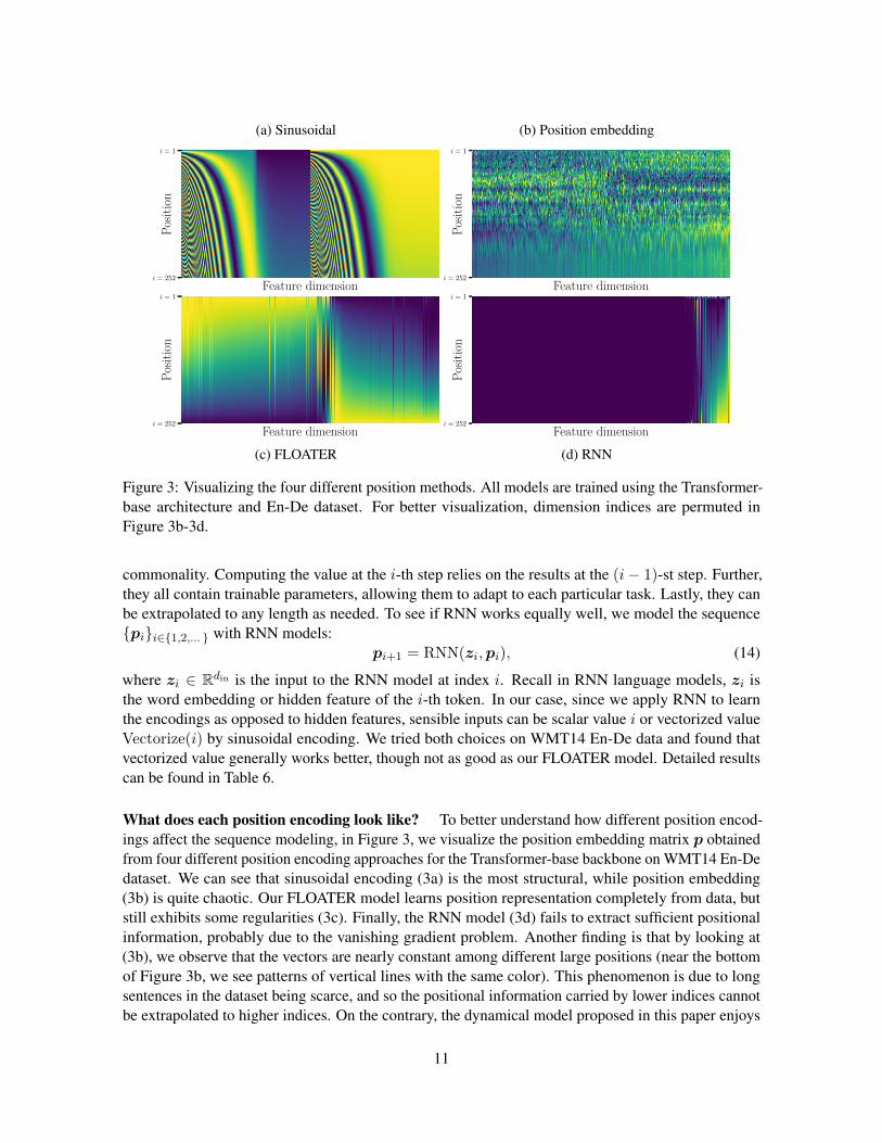
Figure 3: Visualizing the four different position methods. All models are trained using the Transformer-base architecture and En-De dataset. For better visualization, dimension indices are permuted inFigure 3b-3d.

commonality. Computing the value at the i-th step relies on the results at the (i− 1)-st step. Further,they all contain trainable parameters, allowing them to adapt to each particular task. Lastly, they canbe extrapolated to any length as needed. To see if RNN works equally well, we model the sequence{pi}i∈{1,2,... } with RNN models:

pi+1 = RNN(zi,pi), (14)

where zi ∈ Rdin is the input to the RNN model at index i. Recall in RNN language models, zi isthe word embedding or hidden feature of the i-th token. In our case, since we apply RNN to learnthe encodings as opposed to hidden features, sensible inputs can be scalar value i or vectorized valueVectorize(i) by sinusoidal encoding. We tried both choices on WMT14 En-De data and found thatvectorized value generally works better, though not as good as our FLOATER model. Detailed resultscan be found in Table 6.

What does each position encoding look like? To better understand how different position encod-ings affect the sequence modeling, in Figure 3, we visualize the position embedding matrix p obtainedfrom four different position encoding approaches for the Transformer-base backbone on WMT14 En-Dedataset. We can see that sinusoidal encoding (3a) is the most structural, while position embedding(3b) is quite chaotic. Our FLOATER model learns position representation completely from data, butstill exhibits some regularities (3c). Finally, the RNN model (3d) fails to extract sufficient positionalinformation, probably due to the vanishing gradient problem. Another finding is that by looking at(3b), we observe that the vectors are nearly constant among different large positions (near the bottomof Figure 3b, we see patterns of vertical lines with the same color). This phenomenon is due to longsentences in the dataset being scarce, and so the positional information carried by lower indices cannotbe extrapolated to higher indices. On the contrary, the dynamical model proposed in this paper enjoys

11

the best of both worlds – it is adaptive to dataset distribution, and it is inductive to handle sequenceswith lengths longer than the training split.

4.4 Remarks on Training and Testing Efficiency

It is not surprising that during the training time, our flow-based method adds a non-negligible time andmemory overhead; this is because solving the Neural ODE precisely involves ∼100 times forward andbackward propagations of the flow model. Even though we deliberately designed a small flow model(consisting of only two FFN and one nonlinearity layers), stacking them together still increases trainingtime substantially. To make it possible to train big models, we use the following optimizations:• Initialize with pretrained models that do not contain flow-based dynamics, as discussed in Section 3.3.• From (8), we know that if h(·) is close to zero, then the position information diminishes (derived in

appendix). In this way, our model degenerates to the original Transformer. Inspired by this property,we can initialize the FLOATER with smaller weights. Combining with the previous trick, we obtainan informed initialization that incurs lower training loss at the beginning.• We observed that weights in h(·) are more stable and easy to train. Thus, we can separate the

weights of h(·) from the remaining parts of the Transformer model. Concretely, we can 1) cachethe positional bias vectors for some iterations without re-computing, 2) update the weights of flowmodels less frequently than other parts of the Transformer, and 3) update the flow models with alarger learning rate to accelerate convergence.• For the RoBERTa model, we adopt an even more straightforward strategy: we first download a

pretrained RoBERTa model, plug in some flow-based encoding layers, and re-train the encodinglayers on WikiText-103 dataset for one epoch. When finetuning on GLUE datasets, we can chooseto freeze the encoding layers.

Combining those tricks, we successfully train our proposed models with only 20-30% overheadcompared to traditional models, and virtually no overhead when finetuning RoBERTa model on GLUEbenchmarks. Moreover, there is no overhead during the inference stage if we store the pre-calculatedpositional bias vectors in the checkpoints.

5 Conclusions

In this paper, we have shown that learning position encoding with a dynamical model can be anadvantageous approach to improve Transformer models. Our proposed position encoding approachis inductive, data-driven, and parameter efficient. We have also demonstrated the superiority of ourproposed model over existing position encoding approaches on various natural language processingtasks such as neural machine translation, language understanding, and question answering tasks.

References

[1] Ashish Vaswani, Noam Shazeer, Niki Parmar, Jakob Uszkoreit, Llion Jones, Aidan N Gomez,Łukasz Kaiser, and Illia Polosukhin. Attention is all you need. In Advances in Neural InformationProcessing Systems, pages 5998–6008, 2017.

[2] Jacob Devlin, Ming-Wei Chang, Kenton Lee, and Kristina Toutanova. Bert: Pre-training of deepbidirectional transformers for language understanding. arXiv preprint arXiv:1810.04805, 2018.

12

[3] Zhilin Yang, Zihang Dai, Yiming Yang, Jaime Carbonell, Ruslan Salakhutdinov, and Quoc VLe. Xlnet: Generalized autoregressive pretraining for language understanding. arXiv preprintarXiv:1906.08237, 2019.

[4] Alec Radford, Jeff Wu, Rewon Child, David Luan, Dario Amodei, and Ilya Sutskever. Languagemodels are unsupervised multitask learners. 2019.

[5] Zhenzhong Lan, Mingda Chen, Sebastian Goodman, Kevin Gimpel, Piyush Sharma, and RaduSoricut. Albert: A lite bert for self-supervised learning of language representations. arXiv preprintarXiv:1909.11942, 2019.

[6] Colin Raffel, Noam Shazeer, Adam Roberts, Katherine Lee, Sharan Narang, Michael Matena,Yanqi Zhou, Wei Li, and Peter J Liu. Exploring the limits of transfer learning with a unifiedtext-to-text transformer. arXiv preprint arXiv:1910.10683, 2019.

[7] Chulhee Yun, Srinadh Bhojanapalli, Ankit Singh Rawat, Sashank J Reddi, and Sanjiv Kumar.Are transformers universal approximators of sequence-to-sequence functions? arXiv preprintarXiv:1912.10077, 2019.

[8] Yinhan Liu, Myle Ott, Naman Goyal, Jingfei Du, Mandar Joshi, Danqi Chen, Omer Levy, MikeLewis, Luke Zettlemoyer, and Veselin Stoyanov. Roberta: A robustly optimized bert pretrainingapproach. arXiv preprint arXiv:1907.11692, 2019.

[9] Peter Shaw, Jakob Uszkoreit, and Ashish Vaswani. Self-attention with relative position represen-tations. In Proceedings of the 2018 Conference of the North American Chapter of the Associationfor Computational Linguistics: Human Language Technologies, Volume 2 (Short Papers), pages464–468, 2018.

[10] Mostafa Dehghani, Stephan Gouws, Oriol Vinyals, Jakob Uszkoreit, and Łukasz Kaiser. Universaltransformers. arXiv preprint arXiv:1807.03819, 2018.

[11] Tian Qi Chen, Yulia Rubanova, Jesse Bettencourt, and David K Duvenaud. Neural ordinarydifferential equations. In Advances in Neural Information Processing Systems, pages 6571–6583,2018.

[12] Will Grathwohl, Ricky TQ Chen, Jesse Betterncourt, Ilya Sutskever, and David Duvenaud.Ffjord: Free-form continuous dynamics for scalable reversible generative models. arXiv preprintarXiv:1810.01367, 2018.

[13] M. Tenenbaum and H. Pollard. Ordinary Differential Equations: An Elementary Textbook forStudents of Mathematics, Engineering, and the Sciences. Dover Books on Mathematics. DoverPublications, 1985.

[14] Myle Ott, Sergey Edunov, Alexei Baevski, Angela Fan, Sam Gross, Nathan Ng, David Grangier,and Michael Auli. fairseq: A fast, extensible toolkit for sequence modeling. arXiv preprintarXiv:1904.01038, 2019.

[15] Guokun Lai, Qizhe Xie, Hanxiao Liu, Yiming Yang, and Eduard Hovy. Race: Large-scale readingcomprehension dataset from examinations. arXiv preprint arXiv:1704.04683, 2017.

13

[16] Alex Wang, Amanpreet Singh, Julian Michael, Felix Hill, Omer Levy, and Samuel R Bowman.Glue: A multi-task benchmark and analysis platform for natural language understanding. arXivpreprint arXiv:1804.07461, 2018.

[17] Pranav Rajpurkar, Jian Zhang, Konstantin Lopyrev, and Percy Liang. Squad: 100,000+ questionsfor machine comprehension of text. arXiv preprint arXiv:1606.05250, 2016.

[18] Pranav Rajpurkar, Robin Jia, and Percy Liang. Know what you don’t know: Unanswerablequestions for squad. arXiv preprint arXiv:1806.03822, 2018.

[19] William H Press, Saul A Teukolsky, William T Vetterling, and Brian P Flannery. Numericalrecipes in c++. The art of scientific computing, 2:1002, 1992.

[20] Myle Ott, Sergey Edunov, David Grangier, and Michael Auli. Scaling neural machine translation.arXiv preprint arXiv:1806.00187, 2018.

[21] Stephen Merity, Caiming Xiong, James Bradbury, and Richard Socher. Pointer sentinel mixturemodels. arXiv preprint arXiv:1609.07843, 2016.

[22] Yang Liu and Mirella Lapata. Hierarchical transformers for multi-document summarization.arXiv preprint arXiv:1905.13164, 2019.

[23] Xingxing Zhang, Furu Wei, and Ming Zhou. HIBERT: document level pre-training of hierarchicalbidirectional transformers for document summarization. CoRR, abs/1905.06566, 2019.

[24] Tian Qi Chen, Yulia Rubanova, Jesse Bettencourt, and David K Duvenaud. Neural ordinarydifferential equations. In S. Bengio, H. Wallach, H. Larochelle, K. Grauman, N. Cesa-Bianchi,and R. Garnett, editors, Advances in Neural Information Processing Systems 31, pages 6571–6583.Curran Associates, Inc., 2018.

A Training a Neural ODE model in Transformer

We discuss the details of training the dynamical model h(τ,pτ ;wh), recall in our FLOWER model,function h joins in the computational graph implicitly by generating a sequence of position encodingvectors {p1,p2, . . . ,pN}, conditioning on a freely initialized vector p0. The generation steps arecomputed iteratively as follows (suppose we choose the interval between two consecutive tokens to be∆)

p1 = p0 +

∫ ∆

0h(τ,pτ ;wh) dτ,

p2 = p1 +

∫ 2∆

∆h(τ,pτ ;wh) dτ,

...

pN = pN−1 +

∫ N∆

(N−1)∆h(τ,pτ ;wh) dτ.

(15)

Finally, the loss L of this sequence is going to be a function of all position encoding results L =L(p0,p1, . . . ,pN ), which is further a function of model parameters wh. The question is how to

14

calculate the gradient dLdwh

through backpropagation. This question is fully solved in Neural ODEmethod [11] with an efficient adjoint ODE solver. To illustrate the principle, we draw a diagramshowing the forward and backward propagation in Figure 4.

ps pt

L = L(p0 . . . pN) Forward

Backward

+∫ ts h(τ, pτ ;wh)dτ

Figure 4: Direction of forward and backward propagation. Here we consider a simplified version whereonly position encodings ps and pt are in the computational graph.

From [11], we know that the gradients ddwh

L(ps +

∫ ts h(τ,pτ ;wh) dτ

), dL

dwhcan be computed by

dL

dwh= −

∫ s

ta(τ)ᵀ

∂h(τ,pτ ;wh)

∂whdτ, (16)

where a(τ) defined in τ ∈ [s, t] is called the “adjoint state” of ODE, which can be computed by solvinganother ODE

da(τ)

dτ= −a(τ)ᵀ

∂h(τ,pτ ;wh)

∂pτ. (17)

Note that the computation of (17) only involves Jacobian-vector product so it can be efficientlycalculated by automatic differentiation.

B Implementation details

B.1 Settings of ODE solver

To setup the ODE server, we need to first choose the numerical algorithms [19]. We have differentsetups for different datasets. For neural machine translation problems (WMT14 En-De and En-Fr), weuse the more accurate Runge-Kutta scheme with discretization step ∆

5.0 to solve the adjoint equation(recall that we set the interval of two neighboring tokens to be ∆ = 0.1 globally). While for datasetswith long sentences such as GLUE and RACE benchmarks, we found that solving the adjoint equationwith high order scheme is too slow, in such case we adopt simple midpoint method with discretizationstep ∆

5.0 , and the gradients are calculated by automatic differentiation rather than adjoint method. Thethird party implementation of ODE solver can be found at https://github.com/rtqichen/torchdiffeq.

B.2 Training NMT tasks

We run the same preprocessing script provided by fairseq [14], which is also used in ScalingNMT [20].With the standard training script, we first successfully reproduce all the results in Transformer paper [1].Based on that we execute the following protocol to get our results:

15

1. Train the original Transformer model for 30 epochs.

2. Random initialize FLOWER model of same shape configuration.

3. Copy tensors from the best performing checkpoint (validation set) to initialize FLOWER model.Initialize weights in the dynamical model with small values.

4. Half the peak learning rate (e.g. in Transformer-base + En-De, the peak learning rate is changedfrom 7.0× 10−4 to 3.5× 10−4).

5. With the warm-initialized FLOWER checkpoint, retrain on the same dataset for 10 epochs(En-De) or 1 epoch (En-Fr).

6. Averaging last 5 checkpoints and compute BLEU score on test split.

B.3 Training language understanding tasks

For GLUE/SQuAD/RACE benchmarks, our experiments are all conducted upon RoBERTa, in whichboth base and large configurations are available. Due to resource constraint (and to show thecompatibility to existing models), we initialize our FLOWER model with pretrained RoBERTa, whichis similar to NMT task. However, the weightswh in dynamic function h(τ,pτ ;wh) are not trained inlarge corpus, given that GLUE/SQuAD/RACE datasets are too small to train dynamics from scratch,we decided to pretrain h alone in WikiText103 [21] data using masked language modeling loss. Wehave found that when we train wh alone, it only takes a few hours (2x Titan V100) and one epoch toconvergence.Once having the pretrained FLOWER model, we can run following downstream tasks and comparewith RoBERTa under the same setting:

GLUE benchmark consists of eight datasets and each have different hyperparameter settings. Forhyperparameters such as learning rate, batch size, training iterations, warm-up iterations, etc., we usethe same values recommended by official repository of RoBERTa1.

SQuAD benchmark. For this benchmark we wrote our own finetuning code because currently thereis no official code available. During the implementation process, we mainly refer to the third-partyrepositories2. We are not able to exactly match the official result reported in RoBERTa paper butquite close (∼0.1 difference in F1). For our FLOWER model, we use the same hyperparameters asRoBERTa.

RACE benchmark. This benchmark has the longest context and sequence length. We follow theofficial training script3 and reproduce the result. Similar to other benchmarks, we then repeat thetraining process using exactly the same training hyperparameters to make a fair comparison. In thisbenchmark we freeze the weights wh and only finetune the weights of RoBERTa.

1Available at: https://github.com/pytorch/fairseq/blob/master/examples/roberta/README.glue.md

2 Mainly https://github.com/ecchochan/roberta-squad and https://github.com/huggingface/transformers

3https://github.com/pytorch/fairseq/blob/master/examples/roberta/README.race.md

16

C Cases suitable for non-equidistant discritization

Although our model allows continuous values of s and t in (8), limiting the scope to text modeling tasks,positions are discrete values as {0, 1, 2, . . . }. Once the continuous version of position representationpt is obtained, we simply take the discritized {p0,p∆,p2∆, . . . , } as the actual values to feed intoTransformer model, where ∆ is a hyperparameter (e.g. ∆ = 0.1). By choosing positions t equidistantly,we are implicitly assuming the position signal evolves steadily as we go through each token in asentence. More generally, the dynamics in (8) can deal with the case in which positions are not integers0, 1, 2, . . . etc., but arbitrary monotone increasing series t0 < t1 < t2 < . . . which may not beequidistant. In appendix, we exemplify this general situation with several widely deployed tasks; weregard this as a interesting future direction. This makes our model particularly suitable for followingscenarios yet traditional position representation may not be good at:• Hierarchical Transformer model [22, 23]. The model is a direct extension of hierarchical RNN and

is often used in long document processing. It works by first running a word-level Transformer modelon each sentence to extract the sentence embedding, and then applying a sentence-level Transformerscanning through each sentence embedding sequentially. We argue that when processing at thesentence level, it could be better to set the increment of position index ti+1 − ti proportional to thelength of the i-th sentence. This is because longer sentences tend to carry more information, so pi+1

is likely to move farther from pi.• Transformer for time-series events. As measurement time is continuous, time-series data is another

scenario when a continuous position makes more sense than a discrete counterpart. More importantly,to predict the future values by modeling historical values observed at irregular time grids, it is betterto consider the length of time horizon between two consecutive measures. A successful previouswork is the Latent ODE [24], except that they use RNN as the backbone, and they model the hiddenstates rather than position representations with Neural ODE (because RNN itself provides positionalbias).

In this paper, we are not going to explore the more general cases discussed above. Instead, we decidedto leave them as interesting future work.

17