Learning Trans-dimensional Random Fields with Applications

0162-8828 (c) 2016 IEEE. Personal use is permitted, but republication/redistribution requires IEEE permission. See http://www.ieee.org/publications_standards/publications/rights/index.html for more information.

This article has been accepted for publication in a future issue of this journal, but has not been fully edited. Content may change prior to final publication. Citation information: DOI 10.1109/TPAMI.2017.2696536, IEEETransactions on Pattern Analysis and Machine Intelligence

1

Learning Trans-dimensional Random Fields withApplications to Language Modeling

Bin Wang, Student Member, IEEE, Zhijian Ou, Senior Member, IEEE, and Zhiqiang Tan

Abstract—To describe trans-dimensional observations in sample spaces of different dimensions, we propose a probabilistic model,called the trans-dimensional random field (TRF) by explicitly mixing a collection of random fields. In the framework of stochasticapproximation (SA), we develop an effective training algorithm, called augmented SA, which jointly estimates the model parametersand normalizing constants while using trans-dimensional mixture sampling to generate observations of different dimensions.Furthermore, we introduce several statistical and computational techniques to improve the convergence of the training algorithm andreduce computational cost, which together enable us to successfully train TRF models on large datasets. The new model and trainingalgorithm are thoroughly evaluated in a number of experiments. The word morphology experiment provides a benchmark test to studythe convergence of the training algorithm and to compare with other algorithms, because log-likelihoods and gradients can be exactlycalculated in this experiment. For language modeling, our experiments demonstrate the superiority of the TRF approach in beingcomputationally more efficient in computing data probabilities by avoiding local normalization and being able to flexibly integrate aricher set of features, when compared with n-gram models and neural network models.

Index Terms—Language modeling, Random field, Stochastic approximation, Trans-dimensional sampling, Undirected graphicalmodeling.

F

1 INTRODUCTION

G RAPHICAL models [1], [2] have emerged as a general frame-work for describing and applying probabilistic models in

building intelligent systems, and can be broadly classified intotwo classes. In the directed graphical models (also known asBayesian networks), the joint distribution is factorized into aproduct of local conditional density functions, whereas in theundirected graphical models (also known as Markov random fieldsor Markov networks) the joint density function is defined to beproportional to the product of local potential functions. In certainapplications, namely fixed-dimensional settings, the probabilisticmodel specifies a joint distribution over a fixed set of randomvariables, for example, in the modeling of fixed-size images.However, in many other applications, the probabilistic modelrelates to a much more complex sample space, which will be calledthe trans-dimensional setting: the observations can be of differentdimensions. A familiar case is temporal modeling of sequentialdata, where each observation is a sequence of a random length. Itis desirable to build a probabilistic model applicable to sequencesof different lengths.

Currently in the trans-dimensional setting, the directed graph-ical modeling approach, e.g. through hidden Markov models or,more generally, dynamic Bayesian networks, is dominant partic-ularly for sequential data. In contrast, the undirected graphicalmodeling approach is rarely used in the trans-dimensional setting.This is presumably because fitting undirected models is morechallenging than fitting directed models [2]. In general, calculatingthe log-likelihood and its gradient is analytically intractable evenfor fixed-dimensional undirected models, because this involves

• Bin Wang and Zhijian Ou are with the Department of Electronic Engineer-ing, Tsinghua university, Beijing, China. E-mail: [email protected]

• Zhiqiang Tan is with the Department of Statistics, Rutgers University, NJ,USA. Email: [email protected]

evaluating the normalizing constant (also called the partitionfunction in physics) and, respectively, the expectation with respectto the model distribution. It should be noted that the normal-izing constant and model expectation can be exactly calculatedor efficiently approximated under some limited circumstances,mostly in low tree-width1 random fields (e.g. chain-structured)with moderately sized state spaces2. The widely used conditionalrandom fields (CRFs) [3] satisfy these conditions, by only model-ing the conditional distribution over labels given the observations.As a result, CRFs deal with trans-dimensional data but with asignificantly reduced sample space of labels. Indeed, currentlymuch of random field learning is pursued for CRFs. But CRFscan only be used for discriminative tasks, e.g. segmenting andlabeling of natural language sentences or images.

In this paper, we are interested in building random field (RF)models for trans-dimensional observations. The fields can havegreater tree-widths (e.g. 5) and larger sized state spaces (e.g. 104),so that they can capture higher-order interactions inherent in thetrans-dimensional data. Roughly speaking, the main advantagesof undirected modeling over directed modeling are: (1) undirectedmodeling is more natural for certain domains such as relational da-ta, where fixing the directions of edges is awkward in a graphicalmodel, and (2) the undirected representation provides greater flexi-bility and potentially more powerful modeling capacity in avoidinglocal normalization and acyclicity requirements. Eliminating theserequirements allows us to easily encode a much richer set ofpatterns/features which characterize the studied phenomenon.

As remarked in [2], it can be problematic to construct atemplate-based RF model with a certain dimension, and apply

1. The tree-width of a graph is defined as the minimum width over allpossible tree decompositions of the graph, which measures roughly how closethe graph is to a tree. The tree-width of a tree is 1.

2. The state space of a multivariate model is the set of all possible valuesfor each coordinate of a multivariate observation.



2

it to data of a very different dimension. A pioneering work inbuilding RF models for trans-dimensional observations is [4],but the proposed Improved Iterative Scaling (IIS) method forparameter estimation and the Gibbs sampler are not suitable foreven moderately sized RF models. Inducing RF models of Englishword spellings, being sequences of characters, is studied in [4]without numerical evaluation of performances. It is interestingto note that the feature induction and IIS algorithms proposedin [4] are used mostly in later CRF studies. Another previouswork, which is more directly related to our study of RF modelingof trans-dimensional data, is whole-sentence maximum entropy(WSME) language modeling [5]. Language modeling (LM) iscrucial for a variety of computational linguistic applications, suchas speech recognition, machine translation, handwriting recogni-tion, information retrieval and so on. Except the WSME LMs,most LMs follow the directed modeling approach, e.g. n-gramLMs [6], neural network (NN) LMs [7], [8], [9] and conditionalmaximum entropy LMs [10], [11], [12]. Although WSME modelshave the potential benefits of being able to naturally expresssentence-level phenomena and integrate features from a varietyof knowledge sources, their performance results ever reported arenot satisfactory [5], [13], [14] (see Section 2.2). The learningalgorithm used is Generalized Iterative Scaling (GIS) [15] andthe sampling methods for approximating model expectations areGibbs sampling, independence Metropolis-Hasting sampling andimportance sampling [5]. Simple applications of these methodsare hardly able to work efficiently in a trans-dimensional settingespecially with large-size state space3, and hence the WSMEmodels are in fact poorly fitted to the data. This is one of thereasons for the unsatisfactory results of previous WSME models.

To describe trans-dimensional observations, we propose a newprobabilistic model, called the trans-dimensional random field(TRF) model, by explicitly mixing a collection of RFs in samplespaces of different dimensions. With this model formulation,we develop an effective training algorithm in the framework ofstochastic approximation (SA) [16], [17], [18], to jointly estimatethe model parameters and normalizing constants. The trainingalgorithm, which is called augmented SA (AugSA) algorithm,involves two steps, sampling observations and then updating esti-mates of model parameters and normalizing constants, at each it-eration. For the sampling step, we also develop a powerful Markovchain Monte Carlo (MCMC) technique, called trans-dimensionalmixture sampling (TransMS). Furthermore, we introduce severalstatistical and computational techniques, including two-stage con-figuration of learning rates, use of empirical variances to rescaleSA updates, proper specification of dimension probabilities formixture sampling, a modeling strategy to deal with rare high-dimensional observations (e.g. rare long sentences), use of classinformation and multiple CPUs to reduce the computational cost,regularization and stopping decision. All these techniques togetherenable successful training of our TRF models on large datasets.

The TRF modeling approach and the proposed AugSA andTransMS algorithms are thoroughly evaluated in three experi-ments. The first is the word morphology experiment as studied in[4]. Due to the small size of the state space in this experiment,parameter learning can be performed with exactly calculatedlog-likelihoods and gradients. This experiment serves as a validbenchmark to study the convergence of Monte Carlo trainingalgorithms with various configurations. The next two experiments

3. In LMs, the size of state space is the vocabulary size, usually above 104.

are about language modeling, which is our motivating application.We show that TRF LMs significantly outperform n-gram LMs [6],and perform better than recurrent neural network (RNN) LMs [8],[19] and close to Long Short Term Memory (LSTM) LMs [9],[20] but being much faster in computing sentence probabilities.Moreover, interpolated TRF and LSTM LMs produces the lowestword error rate (WER) in speech recognition. We examine thescalability of TRF LMs by incrementally increasing the size ofthe training set and find that they can scale to using training dataof up to 32 million words. All these experiments demonstrate thesuperiority of the TRF models and the effectiveness of the AugSAtraining algorithms. To our knowledge, these results represent thefirst strong empirical evidence supporting the power of using RFapproach to language modeling.

The remainder of this paper is organized as follows. In Section2, we discuss related work. We introduce the TRF model formula-tion in Section 3 and present the training algorithm, AugSA withTransMS, in Section 4. Additional statistical and computationaltechniques for training TRF models are described in Section 5.The experimental evaluations are reported in Sections 6, 7, and 8.We conclude the paper with a discussion in Section 9.

Preliminary part of this work was published in [21]. Newfeatures in this paper include model comparison in Section 3.1,a detailed derivation of the learning algorithm (Section 4.1),an importance sampling extension (Section 4.2, 5.3), simplerconfiguration of learning rates (Section 5.1), a more effectivemethod of rescaling SA update (Section 5.2), dealing with rarehigh-dimensional observations (Section 5.4), stop decision (Ap-pendix D), and extensive new empirical results using new datasetsand “tied” features and providing new comparisons with Adamoptimiser [22], annealed importance sampling (AIS) [23] basedestimates of normalizing constants, and LSTM LMs.

2 RELATED WORK

The central problem addressed in this paper involves buildingRF models for trans-dimensional observations. There are fewdirectly related studies, e.g. [4] and [5]. However, there havebeen many studies of using RF models in the fixed-dimensionalsetting or for discriminative modeling (mainly related to CRFs).In the following, we will briefly discuss these studies and theconnection to our work. Moreover, we further examine relatedwork in language modeling, which is our motivating applicationin trans-dimensional modeling.

2.1 Learning with random fieldsThere is an extensive literature devoted to maximum likelihood(ML) learning of random fields, which is in general difficultbecause calculating the log-likelihood and its gradient is ana-lytically intractable. Roughly speaking, there are two types ofapproximate methods — gradient methods and lower bound meth-ods. The gradient methods make explicit use of the gradient. Animportant class is stochastic approximation methods [16], whichapproximates the model expectations by Monte Carlo sampling forcalculating the gradient. The classic algorithm, initially proposedin [24], is often called stochastic maximum likelihood (SML). Inthe literature on training restricted Boltzmann machines (RBMs),SML is also known as persistent contrastive divergence (PCD)[25] to emphasize that the Markov chain is not reset betweenparameter updates. Among the lower bound methods for MLlearning of random fields, an important class is iterative scaling



3

methods such as GIS [15] and IIS [4]. These algorithms iterativelyoptimize lower bounds of the likelihood function to find themaximum likelihood estimates and are mostly studied in thecontext of maximum entropy (maxent) parameter estimation4 andlogistic regression which is a conditional version of maxent. Inpractice the gradient methods are shown to be much faster thanthe lower bound methods [26], [27].

Remarkably, the above studies are mostly restricted to traininga single fixed-dimensional RF model, and the parameter and thenormalizing constant are estimated separately. Beyond the simpleapplication of SA as in SML, we develop the augmented SAalgorithm for jointly estimating the model parameter and multiplenormalizing constants. Basically, stochastic approximation pro-vides a mathematical framework for stochastically solving a rootfinding problem, which has the form of expectations being equalto zeros [16], [17], [18]. The starting point for augmented SA is toformulate a system of simultaneous equations in this form for boththe maximum likelihood estimates and the normalizing constants.The most relevant previous works that inspire our algorithmicdevelopment are [28] on SA for fitting a single RF, [29] onsampling and estimating normalizing constants from multiple RFsof the same dimension, and [30] on trans-dimensional MCMC.

Finally, it is worthwhile to point out that by only modelingthe conditional distribution over labels given the observations,CRFs deal with trans-dimensional data but with a significantlyreduced sample space of labels. In order for CRFs to be com-putationally tractable, usual CRF formulations are mostly limitedto incorporating pairwise interactions among labels. In order toallow for higher-order interactions, there presents the challenge ofbuilding RF models in the trans-dimensional setting with greatertree-widths, which is the same concern addressed in this paper.

2.2 Language modelingLanguage modeling involves determining the joint probabilityp(x) of a sentence x, which can be denoted as a pair x = (l, xl),where l is the length and xl = (x1, . . . , xl) is a sequence of lwords. Currently, the dominant approach to language modeling isthe directed or conditional modeling, which decomposes the jointprobability of xl into a product of conditional probabilities5 byusing the chain rule,

p(x1, . . . , xl) =l∏

i=1

p(xi|x1, . . . , xi−1).

To avoid degenerate representation of the conditionals, the historyof xi, denoted as hi = (x1, · · · , xi−1), is reduced to equivalenceclasses through a mapping ϕ(hi) with the assumption

p(xi|hi) ≈ p(xi|ϕ(hi)).

Language modeling in this conditional approach consists offinding suitable mappings ϕ(hi) and effective methods to estimatep(xi|ϕ(hi)). A classic example is the traditional n-gram LMswith ϕ(hi) = (xi−n+1, . . . , xi−1). Various smoothing tech-niques are used for parameter estimation [6]. Recently, neuralnetwork LMs, which have begun to surpass the traditional n-gram LMs, also follow the conditional modeling approach, with

4. It can be proved [4] that the maxent distribution is the same as the maxi-mum likelihood distribution from the closure of the set of RF distributions.

5. And the joint probability of x is modeled as p(x) = p(xl)p(⟨EOS⟩|xl),where ⟨EOS⟩ is a special token placed at the end of every sentence. Thus thedistribution of the sentence length is implicitly modeled.

ϕ(hi) determined by a neural network (NN), which can be eithera feedforward NN [7] or a recurrent NN [8], [9].

Remarkably, an alternative approach is used in whole-sentencemaximum entropy (WSME) language modeling [5]. Specifically,a WSME model has the form

p(x;λ) =1

Z(λ)eλ

T f(x). (1)

Here f(x) is a vector of features, which are computable functionsof x such as n-grams conventionally used, λ is the correspondingparameter vector, and Z(λ) =

∑x e

λT f(x) is the global normal-izing constant, which is typically analytically intractable.

While there has been extensive research on conditional LMs,there has been little work on the whole-sentence LMs, mainlyin [5], [13], [14]. Although the whole-sentence approach has thepotential advantage of being able to flexibly integrate a richer setof features, the empirical results of previous WSME LMs are notsatisfactory, almost the same as traditional n-gram LMs. Afterincorporating lexical and syntactic information, a mere relativeimprovement of 1% and 0.4% respectively in perplexity and inWER was reported for the resulting WSME LM [5]. Subsequentstudies of using WSME LMs with grammatical features, as in[13] and [14], reported perplexity improvement above 10% but noWER improvement when using WSME LMs alone.

3 MODEL DEFINITION

Suppose that it is of interest to build random field models formultiple sets of observations of different dimensions, such asimages of different sizes or sentences of different lengths. Denoteby xj an observation in a sample space X j of dimension j,ranging from 1 to m. The space of all observations is then theunion X = ∪m

j=1X j . To emphasize the dimensionality, eachobservation in X can be represented as a pair x = (j, xj), eventhough j is identified as the dimension of xj . By abuse of notation,write f(x) = f(xj) for features of x.

For j = 1, . . . ,m, assume that the observations xj aredistributed from a random field in the form

pj(xj ;λ) =

1

Zj(λ)eλ

T f(xj),

where f(xj) = (f1(xj), f2(x

j), . . . , fd(xj))T is a feature vec-

tor, λ = (λ1, λ2, . . . , λd)T is the corresponding parameter vector,

and Zj(λ) is the normalizing constant:

Zj(λ) =∑xj

eλT f(xj), j = 1, . . . ,m.

For identifiability, assume that no linear combination of the fea-tures fi(xj), i = 1, . . . , d, is a constant function of xj . Moreover,assume that dimension j is associated with a probability πj forj = 1, . . . ,m with

∑mj=1 πj = 1. Therefore, the pair (j, xj) is

jointly distributed as

p(j, xj ;π, λ) = πj pj(xj ;λ) =

πj

Zj(λ)eλ

T f(xj), (2)

where π = (π1, . . . , πm)T .A feature fi(x

j), i = 1, . . . , d, can be any computablefunction of the input xj . For various applications such as lan-guage modeling, the parameters of local potential functions acrosslocations are often tied together [4]. In our current experiments,each feature fi(xj) is defined in the form fi(x

j) =∑

k fi(xj , k),

where fi(xj , k) is a binary function of xj evaluated at position



4

k. In a trigram example, fi(xj , k) equals to 1 if three specificwords appear at positions k to k + 2 and k ≤ j − 2. Thebinary features fi(xj , k) share the same parameter λi for differentpositions k and dimensions j, so called position-independent anddimension-independent. Hence, the feature fi(x

j) indicates thecount of nonzero fi(x

j , k) over k in the observation xj and takesvalues as non-negative integers.

3.1 Comparison between WSME and TRF models

We comment on the connection and difference between WSMEand TRF models. Suppose that we add the dimension features inthe WSME model (1) and obtain

p(j, xj ;λ, ν) =1

Z(λ, ν)eν

T δ(j)+λT f(xj), (3)

where δ(j) = (δ1(j), · · · , δm(j))T denotes the dimension fea-tures such that δl(j) = 1(j = l), f(xj) denotes the ordinaryfeatures as used in both models (1) and (2), ν = (ν1, . . . , νm)T

and λ are the corresponding parameter vectors, and Z(λ, ν) is theglobal normalizing constant

Z(λ, ν) =m∑j=1

∑xj∈X j

eνT δ(j)+λT f(xj) =

m∑j=1

eνjZj(λ). (4)

We show later in Proposition 1 that when both fitted bymaximum likelihood estimation, model (3) is equivalent to model(2) but with different parameterization. The parameters in model(3) are (λ, ν), whereas the parameters in model (2) are (π, λ).Therefore, an important distinction of our TRF approach for trans-dimensional modeling from previous WSME works lies in the useof dimension features, which has significance consequences inboth model definition and model learning.

First, it is clear that model (2) is a mixture of random fields onsubspaces of different dimensions, with mixture weights explicitlyas free parameters. Hence model (2) will be called a trans-dimensional random field (TRF). Moreover, by maximum like-lihood, the mixture weights can be estimated to be the empiricaldimension probabilities (see Proposition 1).

Second, it is instructive to point out that model (1) is essen-tially also a mixture of RFs, but the mixture weights implied arefixed to be proportional to the normalizing constants Zj(λ):

p(j, xj ;λ) =Zj(λ)

Z(λ)· 1

Zj(λ)eλ

T f(xj), (5)

where Z(λ) =∑

x eλT f(x) =

∑mj=1 Zj(λ). Typically the

unknown mixture weights (5) may differ from the empirical lengthprobabilities and also from each other by orders of magnitudes,e.g. 1040 or more in our experiments. As a result, it is very difficultto efficiently sample from model (1), in addition to the fact that thelength probabilities are poorly fitted for model (1). Setting mixtureweights to the known, empirical length probabilities enables us todevelop an effective learning algorithm, as introduced in Section4. Basically, the empirical weights serve as a control device toimprove sampling from multiple distributions [29], [31].

4 MODEL LEARNING

We develop a novel learning algorithm in the SA framework [17],[18] to estimate both the parameters λ and the normalization

constants Z1(λ), . . . , Zm(λ). Equivalently, we estimate the pa-rameters λ and the log ratios of Zj(λ) :

ζ∗j (λ) = logZj(λ)

Z1(λ), j = 1, . . . ,m,

where Z1(λ) is chosen as the reference value such that it canbe calculated exactly. The core ingredients newly designed arethe augmented SA (AugSA) scheme for simultaneously updatingparameters and normalizing constants (Section 4.2) and trans-dimensional mixture sampling (TransMS) (Section 4.3), which isused in the MCMC sampling step of AugSA.

4.1 Maximum likelihood learningSuppose that the training data consist of a subset of nj observa-tions of dimension j, denoted by Dj , for j = 1, . . . ,m. We derivethe maximum likelihood estimates of (π, λ) for model (2).

Proposition 1. For model (2), the maximum likelihood estimate(MLE) of π is π = (π1, . . . , πm)T with πj = nj/n for j =1, . . . ,m. Moreover, the MLE of λ is determined by

p[f ]− pλ[f ] = 0. (6)

Throughout, p[f ] is the expectation of the feature vector f withrespect to the empirical distribution:

p[f ] =1

n

m∑j=1

∑xj∈Dj

f(xj) =m∑j=1

nj

npj [f ],

with pj [f ] = n−1j

∑xj∈Dj f(xj), and pλ[f ] is the expectation

of f with respect to the joint distribution (2), p(j, xj ; π, λ):

pλ[f ] =m∑j=1

πjpλ,j [f ],

with pλ,j [f ] =∑

xj∈X j f(xj)pj(xj ;λ).

Proof. See Appendix A.

Then we demonstrate that maximum likelihood learning ofTRF model (2) and of model (3) are equivalent to each other butwith different parameterization.

Proposition 2. (i) If λ is an MLE of λ in model (2), then (λ, ν)are MLEs of (λ, ν) in model (3), where λ = λ and for a constantc,

eνj = cπje−ζ∗

j (λ), j = 1, . . . ,m. (7)

(ii) If (λ, ν) are MLEs of (λ, ν) in model (3), then Eq. (7) holdsand λ = λ is an MLE of λ in model (2).(iii) In either (i) or (ii), the fitted model (3), p(j, xj ; λ, ν), isidentical to the fitted model (2), p(j, xj ; π, λ).

Proof. See Appendix A.

As suggested by Eq. (7) and motivated by self-adjusted mix-ture sampling in [29], we define the following distribution of(j, xj) on X by a re-parameterization of model (3):

p(j, xj ;λ, ζ) ∝ (πje−ζj )eλ

T f(xj), (8)

where ζ = (ζ1, . . . , ζm)T with ζ1 = 0, and ζj is related to νjthrough eνj = πje

−ζj and can be interpreted as the hypothesizedvalue of the true value ζ∗j (λ). By Proposition 2, after the re-parametrization from (3) to (8), the MLE of λ under model (8)



5

Input: training set1: set initial values λ(0) = (0, . . . , 0)T and

ζ(0) = ζ∗(λ(0))− ζ∗1 (λ(0))

2: for t = 1, 2, . . . , tmax do3: set B(t) = ∅4: set (j(t,0), x(t,0)) = (j(t−1,K), x(t−1,K))

Step I: MCMC sampling5: for k = 1 → K do6: (j(t,k), x(t,k)) = sample((j(t,k−1), x(t,k−1))) (See

Tab.1)7: set B(t) = B(t) ∪ {(j(t,k), x(t,k))}8: end for

Step II: SA updating9: Compute λ(t) based on (16)

10: Compute ζ(t) based on (17) and (18)11: end for

Fig. 1. Augmented stochastic approximation (AugSA)

is also that of λ under model (2), satisfying (6). Moreover, forfixed λ, the MLE of ζj under model (8) is exactly the true valueζ∗j (λ), satisfying

p(j;λ, ζ)− πj = 0, j = 1, . . . ,m. (9)

where

p(j;λ, ζ) =πje

−ζj+ζ∗j (λ)∑m

l=1 πle−ζl+ζ∗l (λ)

is the marginal probability of dimension j under (8). This re-sult can also be verified by solving Eq. (9) directly. Thereare only m − 1 linearly independent equations in (9) because∑m

j=1 p(j;λ, ζ) =∑m

j=1 πj ≡ 1, and so are only m − 1unknowns (ζ2, . . . , ζm) with ζ1 = 0 for fixed λ.

In summary, the MLE of λ (denoted as λ) and the correspond-ing log ratios of normalizing constants ζ∗j (λ), j = 1, . . . ,m, aredetermined jointly from (6) and (9). Both equations (6) and (9)have the form of equating empirical expectations, p[f ] and πj ,with theoretical expectations, pλ[f ] and p(j;λ, ζ), for the ordi-nary features f(·) and the dimension features δ(·) respectively,as similarly found in maximum likelihood estimation of singlerandom field models [2].

4.2 Stochastic approximationStochastic approximation (SA) was first studied in [16]. There hassince been a vast literature on theory, methods, and applicationsof SA [17], [18]. Here we develop an augmented SA algorithmin the SA framework to simultaneously address the two learningobjectives described in Section 4.1.

We first give a brief review of the SA framework. Suppose thatthe objective is to find the solution θ∗ of h(θ) = 0 with

h(θ) = EY∼g(·;θ)[H(Y ; θ)],

where θ ∈ Rd is a parameter vector of dimension d, and Y is anobservation from a probability distribution g(·; θ) depending on θ,and H(Y ; θ) ∈ Rd is a function of Y . For some initial values θ0and Y0, a general SA algorithm is as follows.

Stochastic approximation (SA):

1) Generate Y (t) ∼ K(Y (t−1), ·), where K(·, ·) is aMarkov transition kernel that admits g(·; θ) as the in-variant distribution.

2) Set θ(t) = θ(t−1)+γtAH(Y (t); θ(t−1)), where γt is thelearning rate (also called gain rate) and A is an invertiblematrix (called gain matrix).

During each SA iteration, it is possible to generate a set ofmultiple observations Y by performing the Markov transitionrepeatedly (instead of only one time) and then use the averageof the corresponding values of H(Y ; θ) for updating θ, as shownin the following algorithm. This technique can help reduce thefluctuation due to slow-mixing of Markov transitions.

SA with multiple moves:

1) Set Y (t,0) = Y (t−1,K). For k from 1 to K, generateY (t,k) ∼ K(Y (t,k−1), ·), where K(·, ·) is a Markovtransition kernel that admits g(·; θ) as the invariant dis-tribution.

2) Setθ(t) = θ(t−1) + γtA{ 1

K

∑Y ∈B(t) H(Y ; θ(t−1))},

where B(t) = {Y (t,k)|k = 1, · · · ,K}.

The convergence of SA has been studied under various reg-ularity conditions [17], [18]. For γt = γ0/t

β with γ0 > 0 and1/2 < β ≤ 1, it can be shown that γ−1/2

t (θ(t) − θ∗) convergesin law as t → ∞ to a multivariate normal distribution N(0,Σ).The maximal rate of variance reduction is reached with β = 1.Moreover, if β = 1, then Σ achieves a minimum at γt = 1/t andA = −{∂h(θ∗)/∂θ}−1, resulting in an optimal SA recursion:

θ(t) = θ(t−1) − 1

t

{∂h

∂θ(θ∗)

}−1

H(Y (t); θ(t−1)), (10)

which is reminiscent of Newton’s update for root-finding. How-ever, the optimal SA recursion (10) is, in general, infeasible be-cause ∂h(θ∗)/∂θ is unknown. There are broadly two approachesto achieving asymptotic efficiency. One is to estimate both θ∗

and ∂h(θ∗)/∂θ by stochastic approximation (e.g. [28]). Anotherapproach is to use the trajectory average θ(t) = t−1

∑ti=1 θ

(i),but set the learning rate γt = γ0/t

β decreasing more slowly thanO(t−1) for 1/2 < β < 1 [32]. While a variation of the firstapproach was explored in our previous work [21] (see Section5.2), the second approach was not found to perform satisfactorilyin our preliminary experiments.

We exploit several new ideas in developing SA algorithms forlearning with TRF. To start, we recast (6) and (9) jointly as asystem of simultaneous equations in the form of h(θ) = 0, withθ = (λ, ζ(1)), Y = (j, xj), g(·; θ) = p(j, xj ;λ, ζ) in (8), and

H(Y ; θ) =

(p[f ]− f(xj)δ(1)(j)− π(1)

), (11)

where ζ(1) = (ζ2, . . . , ζm)T , π(1) = (π2, . . . , πm)T andδ(1)(j) = (δ2(j), . . . , δm(j))T with δl(j) = 1(j = l), definedas 1 if j = l and 0 otherwise (see Appendix B). Then the generalSA algorithm can be used to solve (6) and (9) jointly. In thefollowing, we present two further developments, regarding thechoices of design distribution g(·; θ) and disturbance H(Y ; θ)to improve convergence and regading the choice of gain matrix Ato approximate the optimal SA recursion (10).

First, we provide more general choices of g(·; θ) and H(Y ; θ)than (8) and (11) above, such that the system of equations h(θ) =0 remains equivalent to (6) and (9) jointly.



6

Proposition 3. Let π0 = (π01 , . . . , π

0m)T be fixed proportions,

strictly between 0 and 1 and satisfying∑m

j=1 π0j = 1. Define the

following distribution on the space X :

q(j, xj ;λ, ζ) ∝ (π0j e

−ζj )eλT f(xj). (12)

Then (6) and (9) are jointly equivalent to

p[f ]− qλ,ζ [π

π0f ] = 0, (13)

qλ,ζ [δ(1)]− π0(1) = 0, (14)

where qλ,ζ [ππ0 f ] is the expectation of πj

π0jf(xj) and qλ,ζ [δ(1)] is

that of δ(1)(j) under the joint distribution (12). Eqs. (13)–(14) canbe expressed in the form of h(θ) = 0, with g(·; θ) = q(j, xj ;λ, ζ)and

H(Y ; θ) =

(p[f ]− πj

π0jf(xj)

δ(1)(j)− π0(1)

), (15)

where π0(1) = (π0

2 , . . . , π0m)T .

Proof. See Appendix B.

Proposition 3 represents an importance sampling extension ofour previous SA algorithm [21], in allowing the use of dimensionprobabilities different from the empirical ones when generatingthe observation (j, xj) in the SA algorithm. In the special casewhere π0

j = πj for j = 1, . . . ,m, then the choices (12) and (15)for g(·; θ) and H(Y ; θ) reduce to (8) and (11) earlier. See Section4.3 for MCMC sampling from q(j, xj ;λ, ζ), and Section 5.3 forfurther discussion on the choice of π0.

Second, we discuss the choice of gain matrix A as anapproximation of −{∂h(θ∗)/∂θ}−1 in the optimal SA recur-sion (10). For simplicity, we take A as a block-diagonal ma-trix with diagonal blocks (Aλ, Aζ), partitioned according toθ = (λ, ζ(1)). For the update of λ, we set A−1

λ to a diagonalmatrix, σ = diag(σ1, · · · , σd), as a diagonal approximation to∂pλ[f ]/∂λ|λ=λ∗ , where σi is the stratified empirical variance offeature fi for i = 1, . . . , d:

σi =m∑j=1

nj

npj[(fi − pj [fi])

2].

See Section 5.2 for derivation and further discussion. The resultingupdate of λ at iteration t is then

λ(t) = λ(t−1) + γλ,tσ−1

p[f ]− 1

K

∑(j,xj)∈B(t)

πj

π0j

f(xj)

,

(16)where γλ,t is the learning rate of λ (see Section 5.1). For theupdate of ζ , we provide a trans-dimensional extension of theoptimal SA recursion in self-adjusted mixture sampling [29],which is simple and feasible in spite of the fact that such anoptimal scheme is generally infeasible as mentioned above.

Proposition 4. For fixed λ, Eq. (14) can be expressed in theform of h(ζ(1)) = 0 with g(·; ζ(1)) = q(j, xj ;λ, ζ) andH(Y ; ζ(1)) = δ(1)(j) − π0

(1). The optimal gain matrix, Aζ =

−{ ∂∂ζ(1)

h(ζ(1))}−1|ζ=ζ∗(λ), can be shown to satisfy

Aζ H(Y ; ζ(1)) =

(δ2(j)

π02

, . . . ,δm(j)

π0m

)T

− δ1(j)

π01

.

Proof. The result follows from the proof of Theorem 1 in [29].

By Proposition 4, the resulting update of ζ at iteration t is

ζ(t−12 ) = ζ(t−1) + γζ,t

{δ1(B

(t))

π01

, · · · , δm(B(t))

π0m

}T

, (17)

ζ(t) = ζ(t−12 ) − ζ

(t− 12 )

1 , (18)

where ζ(t)1 , the first element of ζ(t), is set to 0 by (18), and γζ,t

is the learning rate of ζ (see Section 5.1), and δl(B(t)) is the

proportion of dimension l appearing in B(t):

δl(B(t)) =

1

K

∑(j,xj)∈B(t)

1(j = l).

We summarize the augmented SA in Fig.1. At the beginning(Step 1), we set λ as a zero vector and we can calculate thetrue normalizing constants because q(j, xj ;λ, ζ) is a uniformdistribution. At each iteration, we first generate K observationsby the trans-dimensional mixture sampling described in Section4.3 (Step 3 to 8), and then update the parameters λ and log ratiosof normalizing constants ζ (Step 9 and 10).

4.3 Trans-dimensional mixture samplingWe describe a trans-dimensional mixture sampling algorithm tosimulate from the joint distribution q(j, xj ;λ, ζ) in (12), whichis used with (λ, ζ) = (λ(t−1), ζ(t−1)) at time t for MCMCsampling in AugSA (Fig.1). The name “mixture sampling” reflectsthe fact that q(j, xj ;λ, ζ) represents a labeled mixture [29],because j is a label indicating that xj is associated with thedistribution pj(x

j ;λ). With fixed (λ, ζ), this sampling algorithmcan be seen as formally equivalent to reversible jump MCMC [30],which was originally proposed for Bayes model determination.

The trans-dimensional mixture sampling algorithm consistsof two steps at each time t: local jump between dimensionsand Markov move of observations for a given dimension. In thefollowing, we denote by j(t−1) and x(t−1) the dimension andobservation before the current sampling, but use the short notation(λ, ζ) for (λ(t−1), ζ(t−1)).

Step I: Local jump. The Metropolis-Hastings method is usedin this step to sample the dimension. Assuming j(t−1) = k, firstwe draw a new dimension j ∼ Γ(k, ·). The jump distributionΓ(k, j) is defined to be uniform in the neighborhood of k:

Γ(k, j) =

1

3, if k ∈ [2,m− 1], j ∈ [k − 1, k + 1]

1

2, if k = 1, j ∈ [1, 2] or k = m, j ∈ [m− 1,m]

0, otherwise(19)

where m is the maximum dimension. Eq. (19) restricts thedifference between j and k to be no more than one. If j = k, weretain the observation x(t−1) and perform the next step directly,i.e. set j(t) = k and x(t) = x(t−1). If j = k + 1 or j = k − 1,the two cases are processed differently.

If j = k + 1, we first draw an element u from a proposaldistribution: u ∼ gk+1(·|x(t−1)). Then we set j(t) = j (= k+1)and x(t) = {x(t−1), u} with probability{

1,Γ(j, k)

Γ(k, j)

q(j, {x(t−1), u};λ, ζ)q(k, x(t−1);λ, ζ)gk+1(u|x(t−1))

}, (20)

where {x(t−1), u} denotes a vector with dimension k + 1 whosefirst k elements are x(t−1) and the last element is u.



7

If j = k − 1, we set j(t) = j (= k − 1) and x(t) = x(t−1)1:k−1

with probability{1,

Γ(j, k)

Γ(k, j)

q(j, x(t−1)1:j ;λ, ζ)gk(x

(t−1)k |x(t−1)

1:j )

q(k, x(t−1);λ, ζ)

}, (21)

where x(t−1)1:j is the first j elements of x(t−1) and x

(t−1)k is the

kth element of x(t−1).In (20) and (21), gk+1(u|xk) can be flexibly specified as

a proper density function in u. In our application, we find thefollowing choice works reasonably well:

gk+1(u|xk) =q(k + 1, {xk, u};λ, ζ)∑w q(k + 1, {xk, w};λ, ζ)

. (22)

where xk is a vector of dimension k, e.g. xk = x(t−1) in (20)and xk−1 = x

(t−1)1:j in (21). In our experiments, the acceptance

rate of local jumps is around 30%, suggesting that good mixing isachieved by the jump process.

Step II: Markov move. After the step of local jump, we obtain

x(t) =

x(t−1) if j(t) = k{x(t−1), u} if j(t) = k + 1

x(t−1)1:k−1 if j(t) = k − 1

(23)

Then we perform (for example) Gibbs sampling on x(t), fromthe first element to the last element. The pseudo-code of trans-dimensional mixture sampling is shown in Algorithm 1 in Tab.1.

5 ALGORITHM OPTIMIZATION

The augmented SA algorithm may still suffer from slow conver-gence, especially when λ is high-dimensional. In this section,we introduce several statistical and computational techniques toimprove the convergence of the augmented SA algorithm andreduce the computational cost.

5.1 Learning ratesAs mentioned in Section 4.2, setting γt = O(t−1) can achieveasymptotic convergence of the SA algorithm. In practice, to accel-erate the initial convergence and improve stability, we introducea two-stage configuration of the learning rates, following thesuggestion of [28] and [29].

We set the learning rates as

γλ,t =

{(tc + tβλ)−1 if t ≤ t0(tc + t− t0 + tβλ

0 )−1 if t > t0,(24)

γζ,t =

{t−βζ if t ≤ t0(t− t0 + t

βζ

0 )−1 if t > t0,(25)

where 0.5 < βλ, βζ < 1, t0 is an burn-in size, and tc is an offsetconstant for the learning rate of λ. These choices are simpler thanin our previous work [21] primarily because a different techniquefor rescaling SA update in λ is used (see Section 5.2). In the firststage (t ≤ t0), a slow-decaying rate of t−β is used to introducelarge adjustments for 0.5 < β < 1. This forces the estimatesλ(t) and ζ(t) to fall reasonably fast to near the true values. Inthe second stage (t > t0), a fast-decaying rate of t−1 is usedaccording to asymptotic theory of SA. The offset tc is introducedto avoid the learning rate of λ being too large in the first severalSA iterations. Typically, t0 is selected to ensure that there is nomore significant adjustment of the log-likelihood observed on thedevelopment set in the first stage.

100 200 300 400 500 600 700 800 900 10000

20

40

60

80

100

120

140

160

180

200

t

nega

tive

log−

likel

ihoo

d

using online estimated varianceusing empirical varianceAdam

Fig. 2. To compare the convergence of SA training using online estimat-ed variances in [21] (green dash line) and using empirical variances inthis paper (red solid line), and Adam method [22] (blue dot line), we plotan example of the scaled negative log-likelihoods on PTB training setalong the iterations.

5.2 Rescaling SA update in λ

In (16), we introduce a diagonal matrix σ to rescale the updatedirection for λ. Here we discuss the rationale for this technique.

For simplicity, consider (13) with only λ unknown and ζ =ζ∗(λ), which leads back to (6) and can be expressed in the formof h(λ) = 0 with

h(λ) = p[f ]− pλ[f ] = p[f ]−m∑j=1

nj

npλ,j [f ].

As mentioned in Section 4.2, the optimal gain matrix A should beA−1 = −∂h(λ∗)/∂λ. By direct calculation, we find

C(λ) = −∂h(λ)

∂λ=

m∑j=1

πj{pλ,j [ffT ]− pλ,j [f ]pλ,j [f ]T },

where pλ,j [ffT ] =

∑xj∈X j pj(x

j ;λ)f(xj)fT (xj). In general,C(λ∗) is unknown and needs to be approximated. One methodis to estimate C(λ∗) along with λ∗ by stochastic approximation[28], as used in our previous paper [21]. In this method, thediagonal elements of matrix C(λ∗) are estimated concurrentlywith λ∗ during SA iterations and a threshold is introduced tocensor the estimates from below6. Alternatively, we propose theuse of empirical variances to approximate C(λ∗). In fact, theempirical stratified covariance matrix is

C =m∑j=1

nj

n{pj [ffT ]− pj [f ]pj [f ]

T },

where pj [fT f ] = n−1j

∑xj∈Dj

f(xj)f(xj)T . If the fitted distri-bution p(j, xj ;λ∗) is close to the empirical distribution p(j, xj),then C provides a reasonable approximation of C(λ∗). Takingthe diagonal elements of C yields the diagonal matrix σ used toobtain the update (16) for λ.

The use of empirical variances to rescale the gradient can alsobe understood from another perspective. For training log-linearmodels, it has been shown that the convergence of gradient-based

6. In our previous paper [21], only about 20% of the components of λ arelarger than the threshold 10−4.



8

TABLE 1Trans-dimensional mixture sampling (TransMS).

The algorithm 1 is the normal version introduced in section 4.3, and the algorithm 2 is the class-based version introduced in Appendix C

Algorithm 1 Algorithm 2

1: function SAMPLE (j(t−1), x(t−1))2: set k = j(t−1)

3: set (j(t), x(t)) = (j(t−1), x(t−1))Step I: Local jump

4: generate j ∼ Γ(k, ·) by (19)5: if j = k + 1 then6:7: generate u ∼ gk+1(·|x(t−1)) by (22)8: set j(t) = j and x(t) = {x(t−1), u} with probability (20)9: end if

10: if j = k − 1 then11: set j(t) = j and x(t) = x

(t−1)1:j with probability (21)

12: end ifStep II: Markov move

13: for i = 1 → j(t) do14:15:16: draw u ∼ q(j(t), {x(t)

1:i−1, ·, x(t)

i+1:j(t)};λ, ζ) by (12)

17: set x(t)i = u

18: end for19: return (j(t), x(t))20: end function

1: function FASTSAMPLE (j(t−1), x(t−1))2: set k = j(t−1)

3: set (j(t), x(t)) = (j(t−1), x(t−1))Step I: Local jump

4: generate j ∼ Γ(k, ·) by (19)5: if j = k + 1 then6: generate c0 ∼ Qk+1(c)7: generate u ∼ gk+1(·|x(t−1), c0) by (35)8: set j(t) = j and x(t) = {x(t−1), u} with probability (20) and (36)9: end if

10: if j = k − 1 then11: set j(t) = j and x(t) = x

(t−1)1:k−1 with probability (21) and (37)

12: end ifStep II: Markov move

13: for i = 1 → j(t) do14: draw c0 ∼ Qi(c)

15: set c(t)i = c0 with probability (34)16: draw u ∼ q(j(t), {x(t)

1:i−1, ·, x(t)

i+1:j(t)};λ, ζ) by (12) with u ∈ A

c(t)i

17: set x(t)i = u

18: end for19: return (j(t), x(t))20: end function

optimization algorithms can be accelerated by normalizing themeans and variances of features [33]. In fact, the update (16) canbe equivalently expressed as

σ1/2λ(t) = σ1/2λ(t−1)+γλ,t

p[g]− 1

K

∑(j,xj)∈B(t)

πj

π0j

g(xj)

,

where g(xj) = σ−1/2f(xj) is the normalized feature vector suchthat the variances of individual features are 1 and σ1/2λ is thecorresponding parameter vector for g.

Compared with estimating C(λ∗) concurrently with λ∗ duringSA iterations in our previous work [21], using empirical variancesto rescale the update direction for λ has two advantages. First,memory cost and computational time are reduced, because σ canbe calculated offline for one time. Second, the empirical variancesσi can be censored from below by a very small threshold, sothat almost all of the components of λ can be updated withoutmodification of the empirical variances. In our experiments, thethreshold is 10−15 and 99.5% of the components of λ are updatedwith non-censored empirical variances. This technique is found toimprove the convergence of the SA training algorithm, as shownin Fig.2. It is worthwhile to compare our method with relatedadaptive stepsize optimisers, such as Adam [22] and RMSProp[34]. They also scale the gradient with curvature informationbut by applying different preconditioners. As shown in Fig.2,our method of preconditioning using the empirical variancesof features in our language modeling experiments shows betterconvergence than Adam which uses a running average of squaredgradients for preconditioning.

5.3 Dimension probabilities π0

Compared with our previous work [21], another new aspect of theaugmented SA algorithm is to allow the dimension probabilitiesπ0j used in the trans-dimensional mixture sampling to differ from

the empirical dimension probabilities πj = nj/n, in order toovercome limitations caused by setting π0

j = πj . The sample sizenj from the training set may be zero for some j, in which case theaugmented SA algorithm will fail with π0

j = 0 because ζj willnot be updated without any observation of dimension j sampled.Moreover, when π0

j is too small for some j, the estimation ofζj would become problematic because the update scheme (17)involves dividing a fraction δj(B

(t)) by π0j .

For illustration, imagine that π0j is 10−5 for some j, and K =

300 observations are drawn at each iteration. If the dimension jappears at least once in sample set B(t), then δj(B

(t)) ≥ 1/300.Then the update to ζj will be at least 300−1/10−5 = 1000/3 in(17) (ignoring the learning rate γζ,t), which can be much largerthan the true value of ζj . Moveover, if j = 1, this will influencethe updates of all (ζ2, . . . , ζm) in (18). To prevent such heavyfluctuations, we need to avoid setting π0

j too small and particularlyto set π0

1 reasonable large.In our experiments, we set

π0j =

max{uj , c}∑mj=1 max{uj , c}

, (26)

where c is a constant (set to 10−5 in our experiments), and

uj =

{nmax/n, if j ≤ jmax

nj/n, if j > jmax

with nmax = maxj nj and jmax = argmaxj nj . The moti-vation for introducing uj above is to make π0

j large for j = 1and for subsequent dimensions j, because the trans-dimensionalmixture sampling algorithm (Tab.1) only permits a dimensionjump from j to j ± 1. In the experiments, we find that this choiceof the dimension probabilities π0

j helps to considerably improvethe accuracy in the estimation of ζ .



9

5.4 Modeling rare high-dimensional observations

Compared with our previous work [21], we propose still anothertechnique to deal with rare very high-dimensional observations(e.g. rare very long sequences), which are often found in largedatasets. For example, the maximum sentence length in Google1-billion word corpus [35] is more than 1000, but the percentageof sentences longer than 100 is about 0.2% in the datasets used inour experiments (Section 8). To reduce the number of sub-modelscorresponding to different dimensions, we set the near maximumdimension m to a medium value (such as 100) and modify the jointdistribution (8) by introducing a special sub-model that capturesall the sequences longer than m as follows:

p(j, xj ;λ, ζ) ∝nm+/n

eζm+

eλT f(xj), j > m, (27)

where ζ = (ζ1, . . . , ζm, ζm+)T with ζ1 = 0 and nm+ is the

number of the sequences longer than m in the training set. Asingle log ratio of normalizing constants ζm+ is used such thatmodel (27) can be seen as model (1) but only for sequenceslonger than m. The augmented SA algorithm can be extendedwith simple modifications. The maximum dimension in trans-dimensional mixture sampling (Tab.1) is set to be slightly largerthan m (specifically m + 2 in our experiments). Then λ is stillupdated by (16), with (j, xj) ∈ B(t) for both j = 1, . . . ,m andj > m. Both (ζ1, . . . , ζm) and ζm+ are updated by (17) and(18), where δm+(B

(t)) = K−1∑

(j,xj)∈B(t) 1(j > m) is theproportion of dimensions greater than m in the sample B(t).

6 APPLICATION: WORD MORPHOLOGY

In this section, we perform a pilot experiment — word morphol-ogy, to exactly evaluate the performance of TRF models andAugSA training algorithms. This is similar with the experimentin [4] but we provide detailed evaluations of performances, whichincludes studying the convergence of the log-likelihood using thetrue normalizing constants, comparing the estimated normalizingconstants with the true ones, and comparing the IIS presented in[4] with our AugSA training algorithm.

The objective of word morphology is to model English wordsas character sequences by assigning probabilities. The training andtest data are extracted from the English Gigaword dataset7. Thetraining set contains 139K different English words. The test setcontains other 15K different English words. The maximum wordlengths in the training and test sets are 25 (i.e. m = 25).

To construct a TRF model (2), we first extract all the characterunigrams, bigrams and trigrams from the training set and definethe following features:

fv(xj) =

j∑i=1

fi,v(xj),

fvw(xj) =

j−1∑i=1

fi,vw(xj),

fvwy(xj) =

j−2∑i=1

fi,vwy(xj),

where xj denotes the word containing j characters (xj1, . . . , x

jj),

v, vw and vwy denote the character unigram, bigram and trigram

7. https://catalog.ldc.upenn.edu/LDC2003T05

observed in the training set, and fi,v , fi,vw and fi,vwy are thecorresponding unigram, bigram and trigram features evaluated atposition i:

fi,v(xj) =

{1 if xj

i = v0 otherwise,

fi,vw(xj) =

{1 if xj

i = v and xji+1 = w

0 otherwise,

fi,vwy(xj) =

{1 if xj

i = v and xji+1 = w and xj

i+2 = y0 otherwise.

The feature set contains fv , fvw, fvwy , fi=0,v , fi=end,v , fi=0,vw,and fi=end,vw, where fi=0,v and fi=end,v denote the unigram vappearing at the beginning and the end of a word; fi=0,vw andfi=end,vw denote the bigram vw appearing at the beginning andthe end of a word8. The total feature number d = 11929. Weperform the augmented SA (Algorithm 1 in Fig.1)9 to train theTRF model. At each iteration, a sample of K = 100 sequences(i.e. words) are generated by trans-dimensional mixture sampling(Section 4.3). We set π0

j = nj/n (denoted by “nj/n”, the redline in Fig.3(b)) or set π0

j as (26) (denoted by “π0”, the green linein Fig.3(b)) to study the effect of proper specification of lengthprobabilities. The learning rates are set as (24) and (25) with tc =100, βλ = 0.8, βζ = 0.6, t0 = 200. The maximum iterationnumber is fixed as tmax = 1000. The techniques introduced inSections 5.4 and Appendices C–E are not used in this experiment.

We implement three existing methods. First is the n-grammodel [6] widely used in language modeling. Here we view anEnglish word as a character sequence and train a 3-gram modelby the Witten-Bell discounting smoothing method (denoted byWB3), using the SRILM toolkit10. This 3-gram model containsthe same set of features with the TRF models introduced above.Second, we apply the improved iterative scaling (IIS) method [4]to train the same TRF model. For comparison with our AugSAalgorithms, at each iteration, we generate K = 100 words ofrandom lengths11 to estimate the model expectations used in IIS.Third, as the expectation pλ[f ] can be calculated exactly in thispilot experiment, we apply the Quasi-Newton method to solveEq. (6) for the TRF model (denoted by Quasi-Newton). Thisprovides the exact result, relative to which different Monte Carlotraining algorithms can be evaluated. For more complex TRFs asin language modeling in Sections 7–8, the Quasi-Newton methodis infeasible because exact calculation of pλ[f ] is intractable.

To study the performances of different methods, we firstplot in Fig.3(a) the scaled negative log-likelihood (NLL) curves,exactly calculated using the true normalizing constants associatedwith the parameter estimates during iterations by AugSA and IISalgorithms for TRF. The NLLs at the final parameter estimates byQuasi-Newton for TRF and by WB3 for n-gram are also shownas flat lines. Several interesting points can be drawn.

First, IIS (blue solid line) performs poorly in this experiment,with NLL diverging from the exact result (black dot line) obtainedby Quasi-Newton. This may be due to an insufficient number

8. Introducing fi=0,v ,fi=end,v ,fi=0,vw ,fi=end,vw is to make TRF mod-els contain the same set of features as the 3-gram model in [6] does.

9. In this experiment, there is no class information and there is no need toaccelerate the sampling using Algorithm 2 in Fig.1 because the alphabet set Ais very small (26 characters).

10. www.speech.sri.com/projects/srilm/11. For sampling in IIS, we first draw length j with the empirical length

probability nj/n. Then Gibbs sampling is performed to generate a sequenceof length j, initialized from the last sequence of the same length.



10

0 200 400 600 800 100021

21.5

22

22.5

23

23.5

24

24.5

25

t

NLL

AugSA − ζ*

AugSA(π0) − ζ*IIS − ζ*WB3Quasi−Newton

(a) NLL on training set

0 5 10 15 20 250

0.02

0.04

0.06

0.08

0.1

0.12

0.14

0.16

j

π j

nj/n

π0

(b) length probabilities

0 200 400 600 800 100021

21.5

22

22.5

23

23.5

24

24.5

25

t

NLL

AugSA − ζ*AugSA − ζAugSA(π0) − ζ*

AugSA(π0) − ζWB3Quasi−Newton

(c) NLL on training set

0 10 20 30 40 50 60 70−0.1

0

0.1

0.2

0.3

0.4

0.5

0.6

ζ*(t)

(ζ(t

)−

ζ*(t)

)/ζ*(

t)

AugSA (t=100)AugSA (t=1000)

AugSA(π0) (t=100)

AugSA(π0) (t=1000)

(d) (ζ(t) − ζ∗(t))/ζ∗(t) against ζ∗(t)

Fig. 3. Word morphology experiment results. (a)(c) plot the scaled negative log-likelihoods (NLLs) on the training set during iterations or at the finalparameter estimates. (b) shows the distribution of nj/n and π0 as discussed in Section 5.3. (d) plots the relative difference of the estimated logratios of normalizing constants ζ(t) and the true ones ζ∗(t) associated with λ(t) at t = 100 and 1000. The legends are interpreted as follows:

• “AugSA” denotes the augmented SA with π0j = nj/n.

• “AugSA(π0)” denotes the augmented SA with π0 set as described in Section 5.3.• “IIS” denotes the improved iterative scaling (IIS) algorithm.• “WB3” denotes the 3-gram models with Witten-Bell discounting smoothing.• “Quasi-Newton” denotes the Quasi-Newton method using the exact gradients.• “ζ∗” or “ζ” after hyphen indicates, respectively, that the NLL is calculated using the true normalizing constants or the estimated normalizing

constants associated with the current parameter estimates.

(K = 100) of draws used for the estimation of the expectationpλ[f ]. In contrast, our AugSA algorithms (red solid and greensolid lines) perform much better (with NLL converging steadily tothe exact result), using the same number of draws per iterationas in IIS. Second, TRF models trained by AugSA algorithmsyield lower NLL and hence outperform the WB3 model (red dotline), using the same set of features. 12 Third, revising lengthprobabilities π0

j from nj/n (red solid line) to (26) (blue solid line)appears to slightly slow the convergence of the log-likelihood. Butsuch a revision leads to more accurate estimation of normalizingconstants and hence of the log-likelihoods as discussed next.Reliable estimation of log-likelihoods for AugSA is important for

12. The log-likelihoods on the test set are virtually the same as those onthe training set for all the methods studied. This is presumably because thetraining and test sets are sufficiently matched in this experiment.

monitoring the progress of training in practical situations whereexact calculation of log-likelihoods is not feasible.

In Fig.3(c), we plot the NLL curves calculated using the truenormalizing constants (solid lines) and the estimated ones (dashlines) associated with the parameter estimates during iterationsby AugSA algorithms. Setting π0 as (26) yields more accurateestimation of the log-likelihoods: the green dash line is closer tothe green solid line than the red dash line to the red solid line. Infact, using π0

j = nj/n leads to systematic overestimation of NLL:the red dash line is always above the red solid line. In addition,Fig.3(d) shows that the log ratios of normalizing constants ζ(t)

estimated by “AugSA(π0)” (green lines) are closer to the trueζ∗(t) than the ζ(t) estimated by “AugSA” (red lines) to ζ∗(t) at,for instance, iteration t = 100 and 1000.



11

TABLE 2Feature definition in TRF LMs

Type Featuresw (w−3w−2w−1w0)(w−2w−1w0)(w−1w0)(w0)c (c−3c−2c−1c0)(c−2c−1c0)(c−1c0)(c0)

ws (w−3w0)(w−3w−2w0)(w−3w−1w0)(w−2w0)cs (c−3c0)(c−3c−2c0)(c−3c−1c0)(c−2c0)

wsh (w−4w0) (w−5w0)csh (c−4c0) (c−5c0)cpw (c−3c−2c−1w0) (c−2c−1w0)(c−1w0)tied (c−9:−6, c0) (w−9:−6, w0)

7 EXPERIMENTS: LANGUAGE MODELING ON PTBCORPUS

In this section, we apply TRF models for language modeling. Weevaluate the performances of different LMs by perplexity13 (PPL)which is a widely used measure of a LM and by speech recognitionword error rate (WER) which quantifies the usefulness of applyinga LM in speech recognition. Compared with our pervious work[21], the new results reported in this section mainly include:(1) introducing a novel feature type, the tied long skip-bigramfeature “tied” [36], which further demonstrates the flexibility ofTRF modeling to use a richer set of features, (2) re-running theexperiments with the newly developed techniques described inSections 5.2, 5.3 and Appendix E to train TRF LMs, (3) obtainingAIS based estimates of normalizing constants for TRF models,and (4) providing comparisons with LSTM LMs in addition ton-gram and RNN LMs.

The training and development datasets are from the WallStreet Journal (WSJ) portion of Penn Treebank (PTB) corpus.In accordance with previous studies [8], sections 0-20 are usedas the training data (about 930K words), sections 21-22 as thedevelopment data (74K) and section 23-24 as the test data (82K).The vocabulary is limited to 10K words, with one special token⟨UNK⟩ denoting words not in the vocabulary. The baseline isn-gram LMs with modified Kneser-Ney smoothing [6], denotedby KNn, which are trained by the SRILM toolkits. We use theRNNLM toolkit14 to train the RNN LM; the number of hiddenunits is 25015. We use the open-source toolkit provided by [20]to train the LSTM LM, which constains 2 hidden layers and eachlayer contains 250 units16. The hyperparameters are tuned to ourbest through a series of pilot experiments.

For our TRF models, we consider a variety of features asshown in Tab.2, mainly based on word and class information. Eachword is deterministically assigned to a single class, by running theautomatic clustering algorithm proposed in [37] on the trainingdataset. In Tab.2, wi, ci, i = 0,−1, . . . ,−5 denote the wordand its class at different position offset i, e.g. w0, c0 denotesthe current word and its class. The word/class n-gram features“w”/“c”, skipping n-gram features “ws”/“cs” [38], higher-orderskipping features “wsh”/“csh”, and the crossing features “cpw”(meaning class-predict-word) are introduced in [21]. In this paper,

13. The perplexity of a dataset is defined to be the exponential of the meannegative log-likelihood of the dataset per-token.

14. http://rnnlm.org/15. Minibatch size = 10, learning rate = 0.1, BPTT steps = 5. 17 sweeps are

performed before stopping, which takes about 25 hours. No word classing isused, since classing in RNNLMs reduces computation but at cost of accuracy[8]. RNNLMs were experimented with varying numbers of hidden units (100-500). The best result from using 250 hidden units is reported.

16. No dropout is used, since overfitting is not observed in training LSTMLMs in this experiment.

TABLE 3The WERs, NLLs and PPLs on the WSJ’92 test data. 10 TRF modelsare trained by 10 independent AugSA runs. The means ± standard

deviations are shown over the 10 TRFs, with four different estimates ofthe normalizing constants. In addition, the results for one of the 10

TRFs are shown. Sep Std/Sm AIS denotes SeparateStandard/Smoothed AIS. “#feat” denotes the feature size (million).

Model WER (%) NLL PPL #featKN5 8.78 97.9 294.4 2.3RNN [8] 7.90 95.6 257.6 5.1LSTM [9] [20] 7.87 98.6 306.3 6.0The best TRF (200 classes) in the previous work [21], usingfeatures “w+c+ws+cs+cpw”AugSA 7.92 ∼96 ∼265 6.410 TRFs (200 classes) trained from 10 independent runs in thiswork, using features “w+c+ws+cs+wsh+csh+tied”AugSA 7.90±0.07 95.3±0.5 252.7±7.3 7.7Sep Std AIS 8.33±0.23 102.3±1.4 380.9±32.4 7.7Sep Sm AIS 7.89±0.09 102.2±1.0 378.9±22.5 7.7Global AIS 7.90±0.07 116.2±10.3 1066.4±889.5 7.7Results for one of the 10 TRFs aboveAugSA 8.03 95.1 250.4 7.7Sep Std AIS 8.41 103.7 412.4 7.7Sep Sm AIS 8.02 103.3 402.9 7.7Global AIS 8.03 122.5 1225.7 7.7Model interpolation with α = 0.5RNN+KN5 8.00RNN+TRF 7.71±0.06LSTM+KN5 8.09LSTM+TRF 7.59±0.06

we further introduce the tied long-skip-bigram features “tied”[36], in which the skip-bigrams with skipping distances from 6to 9 share the same parameter. In this way we can leverage longdistance contexts without increasing the model size. Note that allthe features f(x) in model (2) are constructed from Tab.2 ina position-independent and dimension-independent manner, andonly the features observed in the training data are used.

The AugSA (Algorithm 2 in Fig.1) is used to train theTRF models. The maximum lengths of sentences in the training,development and test sets are 82, which is not very large. Hencethe technique described in Section 5.4 is not needed. All the othertechniques described in Section 5 are applied to train TRF LMs.At each iteration, we generate a sample of K = 300 sentencesof lengths ranging from 1 to 82 (i.e. m = 82). The learningrates γλ and γζ are configured as (24) and (25) respectively withtc = 3000, βλ = 0.8, βζ = 0.6 and t0 = 2000. The lengthprobabilities π0 are set as (26). We use the automatic stop decisiondescribed in Appendix E, with the L2 regularization constantµ = 4 × 10−5 in (38). We calculate St with H = 100 and stopiteration if St < 10−4. Eight CPU cores are used to parallelize thealgorithm, as described in Appendix D. We also implement the IISmethod for the language modeling experiments17. But the resultsare unsatisfactory, being similar to those in the word morphologyexperiment, and hence are not shown.

For evaluations in terms of speech recognition WERs, variousLMs obtained using PTB training and development datasets areused to re-score 1000-best lists from recognizing WSJ’92 test data(330 utterances). For each utterance, we obtain a 1000-best list ofcandidate sentences by the first-pass recognition using the Kaldi

17. The IIS method is incapable of estimating normalizing constants thatare needed for evaluating LMs. Similarly as in [29], we apply AugSA toestimate the log normalizing constants ζ through (17)–(18), while fixing λ atthe parameter estimates obtained by IIS.



12

5 10 15 20 25 300

50

100

150

200

250

length j

logZj

Log AIS weightsStandard AISSmoothed AISAugSA

Fig. 4. Log normalization constants estimated by different methods forone of the 10 TRFs, whose WER and PPL result are shown in Tab.3.Dots represent the log weights from the 10 chains used to compute theAIS estimates (solid red line).

toolkit18 with a DNN-based acoustic model. The oracle WER ofthe 1000-best lists is 0.93%.

The results on WSJ’92 test set are shown in Tab.3. As thenormalizing constants for TRF models are estimated stochasticallythrough ζj , we report PPLs and WERs over 10 independentAugSA training runs. The TRF LMs are compared against theKN n-gram LMs, the RNN LMs [8], the LSTM LMs [9] and theprevious results in [21]19. We provide the following comments.

First, in addition to various features used in [21], we intro-duce the tied skip-bigram features to further demonstrate TRF’sflexibility in feature integration which may be difficult for neuralnetwork LMs. The resulting TRF LM reduce the WER to about7.90, which outperforms the KN5 LMs significantly with 10%relative reduction. This result is close to the RNN LM and LSTMLM, which show little difference in this experiment.

Second, we examine how the TRF LMs are complimentary toneural network LMs through model interpolation. The sentencelog-probabilities from two models are log-linearly combined withinterpolation weights 0 < α < 1 and 1 − α respectively. Inter-polated TRF and LSTM LMs (LSTM+TRF) produces the lowestWER. Numerically, the relative reduction is 13.6% compared withthe KN5 LM, and 3.2% compared with the single LSTM LM.

Third, for training cost, the single-run training times for TRF,RNN and LSTM are about 20 hours on CPUs, 25 hours on CPUsand 1 hours on GPUs respectively. For testing cost, comparedwith neural network LMs, TRF models are computationally moreefficient in computing sentence probabilities, by simply summingup weights for the activated features in each sentence. The neuralnetwork LMs suffer from the expensive softmax computation inthe output layer 20. Empirically in our experiments, the averagetime costs for re-ranking the 1000-best list of candidate sentencesfor each utterance are 0.16 seconds, 40 seconds and 10 seconds,based on TRF (using CPU), RNN (using CPU) and LSTM (usingGPU) respectively. In our experiments, the RNN and LSTM usedthe softmax version without classing to achieve good accuracy [8].According to a recent paper [40], an advanced implementation

18. http://kaldi.sourceforge.net/19. The WSME LMs (1) using the same sets of features as the TRF LMs

were also evaluated on this dataset. But the WERs and PPLs of the WSMELMs were even worse than the baseline KN5. See the numerical results anddiscussions in the previous work [21].

20. This deficiency could be partly alleviated with some speed-up methods,e.g. using word clustering [19] or noise contrastive estimation [39].

using class-based softmax can achieve a speed-up from 2 to 10times, but that would still be much slower than TRF.

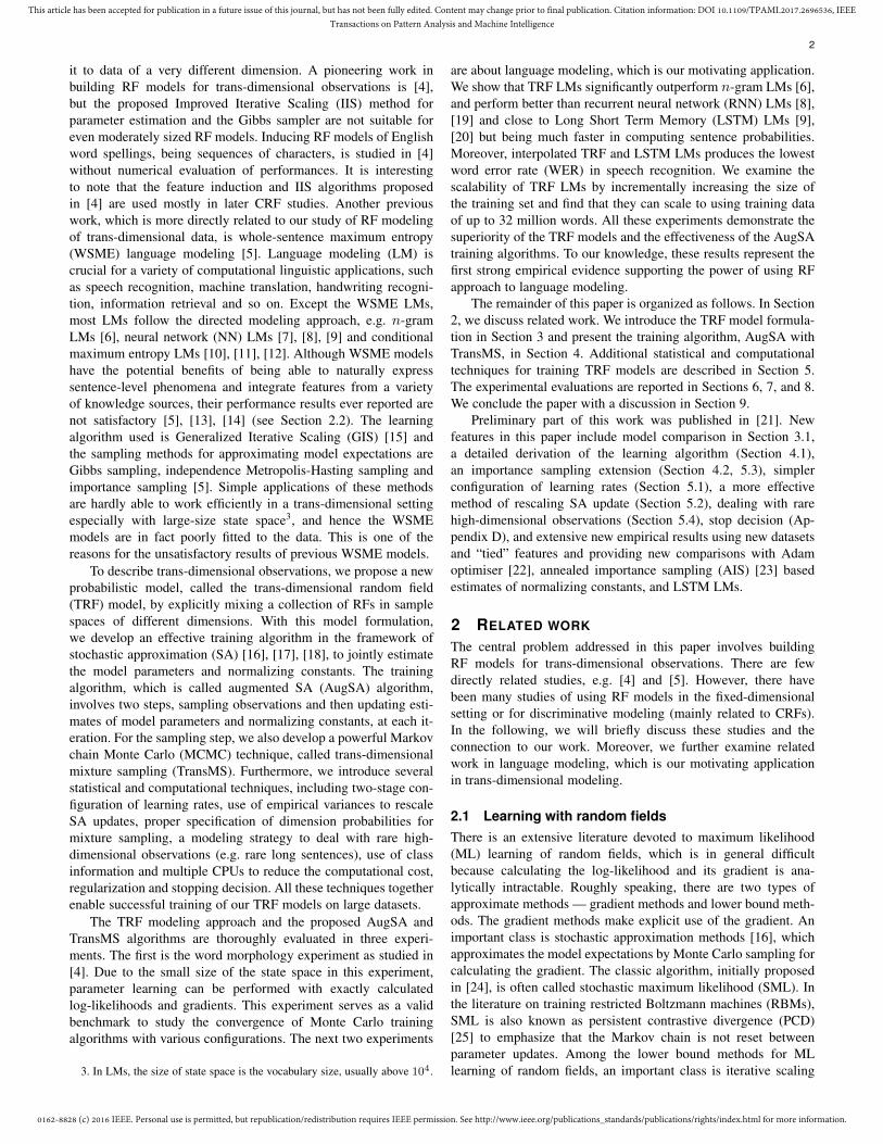
Fourth, as suggested by a referee, we run the AIS method to re-estimate the normalization constants for 10 TRFs obtained from10 independent AugSA runs. There are two approaches. Firstly,by the definition (2), each TRF involves multiple normalizingconstants for different dimensions, which can be estimated by AISseparately over individual fixed-dimensional subspaces. Secondly,each TRF together with the normalizing constants estimated byAugSA can also be viewed as model (3) with a single, globalnormalizing constant, which can be estimated by applying AISover the trans-dimensional state space. Due to the use of estimatednormalizing constants, the two approaches are not equivalent.For the first approach, an AIS run for estimating a normalizingconstant consists of 10 chains with 20K intermediate distributions,and the base distribution is set by zeroing all λ’s. Since themaximum length in the 1000-best lists is 33, we estimate 33normalization constants for lengths from 1 to 33 by 33 AIS runsfor each TRF, which takes about 24 hours (even parallelizing thecomputation over lengths and chains using eight CPUs). Due tothe independence of AIS runs, there are large oscillations in thestandard AIS estimates across different lengths, as shown in Fig.4(red curve). The resulting rescoring performance appears to beworsened by such non-smooth estimates of normalizing constants.To mitigate this defect, for each of the 10 TRFs, we apply a linearregression over the log AIS estimates at 33 sentence lengths toobtain smoothed estimates of normalizing constants, which arethen used to rescore the 1000-best lists. This method, denoted by“Sep Sm AIS” in contrast with “Sep Std AIS”, gives WERs closeto those obtained by AugSA, albeit with substantial extra time cost(about 24 hours for each TRF). While there are some differencesbetween the AugSA and AIS estimates of normalizing constants,it is reassuring and serves as independent validation of the resultsthat both estimates lead to similar WERs after a correction forthe non-smoothness of standard AIS estimates. For the secondapproach, denoted by “Global AIS”, an AIS run for estimating theglobal normalizing constant in (3) contains 10 chains with 200Kintermediate distributions, which takes about 8 hours (parallelizingover chains on ten CPUs) for each TRF. The base distribution isdefined by zeroing all λ’s and then setting ν based on true ζ∗.The rescoring performance is not changed by the global constant,although the log-likelihoods and PPLs are affected.

8 EXPERIMENTS: LANGUAGE MODELING WITHTRAINING DATA OF UP TO 32 MILLION WORDS

In this section, we show the scalability of TRF LMs with theAugSA training algorithm to handle tens of millions of features.The experiments are performed on part of Google 1-billion wordcorpus21. The whole training corpus contains 99 files and each filecontains about 8M words. The whole held-out corpus contains 50files and each file contains about 160K words. In our experiments,we choose the first and second file (i.e. “news.en.heldout-00000-of-00050” and “news.en.heldout-00001-of-00050”) in the held-out corpus as the development set and test set respectively, andincrementally increase the training set as used in our experiments.

First, we use one training file (about 8 million words) asthe training set. We extract the 20K most frequent words from

21. https://github.com/ciprian-chelba/1-billion-word-language-modeling-benchmark



13

TABLE 4The perplexities (PPL) of various LMs with different sizes of trainingdata (8M, 16M, 32M) from Google 1-billion word corpus. The cutoffsettings of n-gram LMs are 0002 (KN4), 00002 (KN5) and 000002

(KN6). The RNN [8] and LSTM [20] are configured the same as in thePTB experiment, except RNN uses 200 classes. The feature type of

TRF is “w+c+ws+cs+wsh+csh+tied”. “#feat” is the feature size (million).

models 8M 16M 32MPPL #feat PPL #feat PPL #feat

KN5 128 18.1 112 33.6 99 61.8RNN 110 9.0 99 9.0 92 9.0

LSTM 82 9.9 73 9.9 68 9.9TRF ∼110 17.5 ∼98 29.2 ∼91 48.7

the training set to construct the lexicon22. Then for the training,development and test set, all the words out of the lexicon aremapped to an auxiliary token <UNK>. The word clusteringalgorithm in [37] is performed on the training set to clusterthe words into 200 classes. We train a TRF model with featuretype “w+c+ws+cs+wsh+csh+tied” (Tab.2). Then we increase thetraining size to around 16 million words (2 training files). We stillextract the 20K most frequent words from the current trainingset to construct a new lexicon. After re-clustering the wordsinto 200 classes, a new TRF model with the same feature type“w+c+ws+cs+wsh+csh+tied” is trained over the new training set.We repeat the above process and train the third TRF model on 32million words (4 training files).

In this experiment, the maximum lengths of sentences in thetraining, development and test sets are more than 1000. Thepercentages of sentences longer than 100 are all about 0.2% in thetraining, development and test sets. Hence we apply the techniquedescribed in Section 5.4, with the near maximum dimension set tom = 100. At each iteration, we generate a sample of K = 300sentences of lengths ranging from 1 to 102. The learning ratesγλ and γζ are configured as (24) and (25) respectively withtc = 1000, βλ = 0, βζ = 0.6 and t0 = 2000. The lengthprobabilities π0 are set as (26). In this experiment, we fix theiteration number tmax = 50, 000 and the L2 regularizationconstants 10−5 to sufficiently train our TRF LMs. Twelve CPUcores are used to parallelize the training algorithm.

The perplexities on the test set are shown in Tab.4. TheWERs obtained from applying various LMs to rescore the WSJ’921000-best list are shown in Tab.5. These results show that theTRF LMs can scale to using training data of up to 32 millionwords. The TRF LMs outperforms the KN5 LMs significantlyin terms of both PPLs and WERs. Compared with the RNNLMs, the TRF LMs give close PPLs but smaller WERs. TheLSTM LMs alone performs better than TRF LMs, but interpolatedTRF and LSTM LMs produces the lowest WER. Numerically,“LSTM+TRF” trained on 32M training corpus achieves 6.33%WER, which represents 17.4% relative reduction over KN5, 5.4%over LSTM and 4.0% over “LSTM+KN5”.

9 CONCLUSION AND FUTURE DIRECTIONS

The undirected graphical modeling approach is rarely used to de-scribe trans-dimensional observations but has its own merits: beingmore natural for domains where fixing the directions of edgesis awkward, being computationally more efficient in computingdata probabilities by avoiding local normalization, and being able

22. After converting all the words to upper case, the vocabulary size isreduced to about 18K.

TABLE 5The WERs on WSJ’92 test set, continuing from Tab.4. The interpolation

weight α is tuned from 0.1 to 0.9 per 0.1.

models 8M 16M 32MKN5 8.24 8.26 7.66RNN 7.47 7.73 7.73

LSTM 7.19 6.88 6.69TRF 7.08 7.17 7.10

RNN+KN5 7.60 7.66 7.43LSTM+KN5 7.14 6.82 6.59RNN+TRF 7.08 7.27 6.93

LSTM+TRF 6.76 6.72 6.33

to flexibly integrate a richer set of features. In this paper, weinvestigate building RF models for trans-dimensional observationsand make the following contributions. (1) We propose the TRFmodel and develop the AugSA training algorithm, which jointlyestimates the model parameters and normalizing constants whileusing trans-dimensional mixture sampling. (2) Several statisticaland computational innovations are introduced to improve the train-ing convergence and reduce computational cost, which togetherenable us to successfully train TRF models on large datasets. (3)The new TRF model and AugSA training algorithm are thoroughlyevaluated. The superiority of the TRF approach is demonstratedin language modeling experiments. The TRF models obtainedsignificantly outperform the classic n-gram LMs and performcompetitive with NN LMs but being much faster in calculatingsentence probabilities.

There are various worthwhile directions for future research.First, the TRF approach will hopefully open a new door tolanguage modeling in addition to the dominant conditional ap-proach, as once envisioned in [5]. Apart from its success inlanguage modeling, the TRF approach can also be applied to othersequential and trans-dimensional data modeling tasks in general.Second, although this work models trans-dimensional observation-s using the log-linear form and without hidden variables, it is animportant direction of extending TRF models to introduce non-linear features (e.g. implemented by NNs) and hidden variablesto further enhance their representational power. Third, anotherimportant line of extension arises by applying the TRF approachto discriminative modeling, even though we are mainly concernedwith generative modeling of trans-dimensional data in this work.The conditional distributions over labels given the observations inCRFs can be described by TRFs so that higher-order interactionsamong labels can be utilized. Finally, to facilitate future studiesalong the TRF approach, we have released an open-source TRFtoolkit23, which contains the code and scripts to reproduce theresults in this paper.

10 ACKNOWLEDGMENTS

This work is partly supported by NSFC grant 61473168, TsinghuaInitiative 20121088069 and Toshiba Corporation.

REFERENCES

[1] B. J. Frey and N. Jojic, “A comparison of algorithms for inference andlearning in probabilistic graphical models,” IEEE Trans. Pattern Analysisand Machine Intelligence (PAMI), vol. 27, no. 9, pp. 1392–1416, 2005.

[2] D. Koller and N. Friedman, Probabilistic graphical models: principlesand techniques. MIT press, 2009.

23. https://github.com/wbengine/SPMILM/



14

[3] J. Lafferty, A. McCallum, and F. Pereira, “Conditional random fields:Probabilistic models for segmenting and labeling sequence data,” Proc.International Conference on Machine Learning (ICML), pp. 282–289,2001.

[4] S. D. Pietra, V. D. Pietra, and J. Lafferty, “Inducing features of randomfields,” IEEE Trans. Pattern Analysis and Machine Intelligence (PAMI),vol. 19, pp. 380–393, 1997.

[5] R. Rosenfeld, S. F. Chen, and X. Zhu, “Whole-sentence exponential lan-guage models: a vehicle for linguistic-statistical integration,” ComputerSpeech & Language, vol. 15, pp. 55–73, 2001.

[6] S. F. Chen and J. Goodman, “An empirical study of smoothing techniquesfor language modeling,” Computer Speech & Language, vol. 13, pp. 359–394, 1999.

[7] H. Schwenk, “Continuous space language models,” Computer Speech &Language, vol. 21, pp. 492–518, 2007.

[8] T. Mikolov, S. Kombrink, L. Burget, J. H. Cernocky, and S. Khudanpur,“Extensions of recurrent neural network language model,” in Proc.International Conference on Acoustics, Speech and Signal Processing(ICASSP), 2011.

[9] M. Sundermeyer, R. Schluter, and H. Ney, “Lstm neural networks forlanguage modeling.” in Proc. Interspeech, 2012, pp. 194–197.

[10] S. Khudanpur and J. Wu, “Maximum entropy techniques for exploitingsyntactic, semantic and collocational dependencies in language model-ing,” Computer Speech & Language, vol. 14, pp. 355–372, 2000.

[11] B. Roark, M. Saraclar, M. Collins, and M. Johnson, “Discriminativelanguage modeling with conditional random fields and the perceptronalgorithm,” in Proc. Ann. Meeting of the Association for ComputationalLinguistics (ACL), 2004, p. 47.

[12] S. F. Chen, “Shrinking exponential language models,” in Proc. HumanLanguage Technologies: Ann. Conference of the North American Chapterof the Association for Computational Linguistics, 2009.

[13] F. Amaya and J. M. Benedı, “Improvement of a whole sentence maxi-mum entropy language model using grammatical features,” in Proc. Ann.Meeting of the Association for Computational Linguistics (ACL), 2001.

[14] T. Ruokolainen, T. Alumae, and M. Dobrinkat, “Using dependencygrammar features in whole sentence maximum entropy language modelfor speech recognition.” in Baltic HLT, 2010.

[15] J. N. Darroch and D. Ratcliff, “Generalized iterative scaling for log-linearmodels,” The Annals of Mathematical Statistics, pp. 1470–1480, 1972.

[16] H. Robbins and S. Monro, “A stochastic approximation method,” TheAnnals of Mathematical Statistics, pp. 400–407, 1951.

[17] A. Benveniste, M. Metivier, and P. Priouret, Adaptive algorithms andstochastic approximations. New York: Springer, 1990.

[18] H. Chen, Stochastic approximation and its applications. SpringerScience & Business Media, 2002.

[19] T. Mikolov, “Statistical language models based on neural networks,”Ph.D. thesis, Brno University of Technology, 2012.

[20] W. Zaremba, I. Sutskever, and O. Vinyals, “Recurrent neural networkregularization,” arXiv preprint arXiv:1409.2329, 2014.

[21] B. Wang, Z. Ou, and Z. Tan, “Trans-dimensional random fields forlanguage modeling,” in Proc. Annu. Meeting of the Association forComputational Linguistics (ACL), 2015.

[22] D. Kingma and J. Ba, “Adam: A method for stochastic optimization,”arXiv:1412.6980 [cs.LG], 2014.

[23] R. M. Neal, “Annealed importance sampling,” Statistics and Computing,vol. 11, no. 2, pp. 125–139, 2001.

[24] L. Younes, “Parametric inference for imperfectly observed gibbsianfields,” Probability Theory and Related Fields, vol. 82, pp. 625–645,1989.

[25] T. Tieleman, “Training restricted boltzmann machines using approxima-tions to the likelihood gradient,” in Proc. International Conference onMachine Learning, 2008.

[26] R. Malouf, “A comparison of algorithms for maximum entropy parameterestimation,” in Proc. Conference on Natural Language Learning (CoNL-L), 2002.

[27] T. P. Minka, “A comparison of numerical optimizers for logistic regres-sion,” Technical report, MSR, 2003.

[28] M. G. Gu and H.-T. Zhu, “Maximum likelihood estimation for spatialmodels by markov chain monte carlo stochastic approximation,” Journalof the Royal Statistical Society: Series B (Statistical Methodology),vol. 63, pp. 339–355, 2001.

[29] Z. Tan, “Optimally adjusted mixture sampling and locally weightedhistogram analysis,” Journal of Computational and Graphical Statistics,vol. 26, pp. 54–65, 2017.

[30] P. J. Green, “Reversible jump markov chain monte carlo computation andbayesian model determination,” Biometrika, vol. 82, pp. 711–732, 1995.

[31] F. Liang, C. Liu, and R. J. Carroll, “Stochastic approximation in montecarlo computation,” Journal of the American Statistical Association, vol.102, no. 477, pp. 305–320, 2007.

[32] B. T. Polyak and A. B. Juditsky, “Acceleration of stochastic approxima-tion by averaging,” SIAM Journal on Control and Optimization, vol. 30,pp. 838–855, 1992.

[33] S. Wiesler and H. Ney, “A convergence analysis of log-linear training,”in Advances in Neural Information Processing Systems, 2011.

[34] T. Tieleman and G. Hinton, “Lecture 6.5-rmsprop: Divide the gradientby a running average of its recent magnitude,” COURSERA: NeuralNetworks for Machine Learning, 2012.

[35] C. Chelba, T. Mikolov, M. Schuster, Q. Ge, T. Brants, P. Koehn, andT. Robinson, “One billion word benchmark for measuring progress instatistical language modeling,” arXiv preprint arXiv:1312.3005, 2013.

[36] N. Shazeer, J. Pelemans, and C. Chelba, “Sparse non-negative matrixlanguage modeling for skip-grams,” in Proc. INTERSPEECH, 2015.

[37] S. Martin, J. Liermann, and H. Ney, “Algorithms for bigram and trigramword clustering,” Speech Communication, vol. 24, pp. 19–37, 1998.

[38] J. Goodman, “A bit of progress in language modeling,” Computer Speech& Language, vol. 15, pp. 403–434, 2001.

[39] A. Mnih and K. Kavukcuoglu, “Learning word embeddings efficientlywith noise-contrastive estimation,” in Proc. Neural Information Process-ing Systems (NIPS), 2013.

[40] E. Grave, A. Joulin, M. Cisse, D. Grangier, and H. Jegou, “Efficientsoftmax approximation for gpus,” arXiv preprint arXiv:1609.04309,2016.

[41] J. Goodman, “Classes for fast maximum entropy training,” in Proc.International Conference on Acoustics, Speech, and Signal Processing(ICASSP), 2001.

[42] G. Hinton, “A practical guide to training restricted boltzmann machines,”Momentum, vol. 9, p. 926, 2010.

Bin Wang received the B.S. degree in electronicengineering from Tsinghua University in 2012.Since 2012, he has been pursuing a Ph.D. de-gree at the Department of Electronic Engineer-ing in Tsinghua University under the supervisionof Zhijian Ou. From April 2015 to September2015, he was a visiting student and worked withZhiqiang Tan at the Department of Statisticsin Rutgers University. His research focuses ontrans-dimensional random fields and languagemodeling.

Zhijian Ou received the B.S. degree with thehighest honor in electronic engineering fromShanghai Jiao Tong University in 1998 andthe Ph.D. degree in electronic engineering fromTsinghua University in 2003. Since 2003, hehas been with the Department of Electron-ic Engineering in Tsinghua University and iscurrently an associate professor. From August2014 to July 2015, he was a visiting schol-ar at Beckman Institute, University of Illinoisat Urbana-Champaign. He has actively led re-

search projects from NSF China (NSFC), China 863 High-tech Re-search and Development Program, and China Ministry of InformationIndustry, as well as joint-research projects with Intel, Panasonic, IBM,and Toshiba. His recent research interests include speech processing(speech recognition and understanding, speaker recognition, naturallanguage processing) and machine intelligence (particularly with graph-ical models).

Zhiqiang Tan is a Professor with the Depart-ment of Statistics at Rutgers University. He re-ceived the B.S. degree in applied mathematicsfrom Tsinghua University in 1998 and the Ph.D.degree in statistics from University of Chicago in2003. He was an Assistant Professor at JohnsHopkins University from 2003 to 2007 beforejoining Rutgers University. He received an NSFCAREER award in 2007, and became an Elect-ed Member of International Statistical Institute in2015. He has published extensively on statistical

theory, methods, and applications in leading statistical and interdisci-plinary journals and conferences. His research interests include MonteCarlo methods, causal inference, statistical learning, and related areas.

Documents

Learning Trans-dimensional Random Fields with Applications