Embed Size (px)
Citation preview
Journal of Machine Learning Research 11 (2010) 1353-1390 Submitted 3/09; Revised 12/09; Published 4/10
Learning Translation Invariant Kernels for Classification
Kamaledin Ghiasi-Shirazi [email protected] Safabakhsh [email protected] Engineering DepartmentAmirkabir University of TechnologyTehran, 15914, Iran
Mostafa Shamsi M [email protected] of Mathematics and Computer ScienceAmirkabir University of TechnologyTehran, 15914, Iran
Editor: John Shawe-Taylor
AbstractAppropriate selection of the kernel function, which implicitly defines the feature space of an algo-rithm, has a crucial role in the success of kernel methods. Inthis paper, we consider the problemof optimizing a kernel function over the class of translation invariant kernels for the task of binaryclassification. The learning capacity of this class is invariant with respect to rotation and scaling ofthe features and it encompasses the set of radial kernels. Weshow that how translation invariantkernel functions can be embedded in a nested set of sub-classes and consider the kernel learningproblem over one of these sub-classes. This allows the choice of an appropriate sub-class basedon the problem at hand. We use the criterion proposed by Lanckriet et al. (2004) to obtain a func-tional formulation for the problem. It will be proven that the optimal kernel is a finite mixture ofcosine functions. The kernel learning problem is then formulated as a semi-infinite programming(SIP) problem which is solved by a sequence of quadraticallyconstrained quadratic programming(QCQP) sub-problems. Using the fact that the cosine kernel is of rank two, we propose a formula-tion of a QCQP sub-problem which does not require the kernel matrices to be loaded into memory,making the method applicable to large-scale problems. We also address the issue of includingother classes of kernels, such as individual kernels and isotropic Gaussian kernels, in the learningprocess. Another interesting feature of the proposed method is that the optimal classifier has anexpansion in terms of the number of cosine kernels, instead of support vectors, leading to a remark-able speedup at run-time. As a by-product, we also generalize the kernel trick to complex-valuedkernel functions. Our experiments on artificial and real-world benchmark data sets, including theUSPS and the MNIST digit recognition data sets, show the usefulness of the proposed method.
Keywords: kernel learning, translation invariant kernels, capacitycontrol, support vector ma-chines, classification, semi-infinite programming
1. Introduction
Kernel-based methods, such as support vector machines (SVM) and kernel principal componentanalysis (KPCA), increase the flexibility of machine learning algorithms by implicitlymappingthe input data into a feature space and performing the algorithm in that space. This flexibility isachieved by a so called kernel function which substitutes the dot-productoperation in an ordinaryalgorithm. The kernel function, by implicitly defining the feature space, playsa crucial role in the
c©2010 Kamaledin Ghiasi-Shirazi, Reza Safabakhsh and MostafaShamsi.

GHIASI-SHIRAZI , SAFABAKHSH AND SHAMSI
success of kernel methods. In fact, as shown by Xiong et al. (2005),if the kernel function is notchosen appropriately, it may even worsen the performance of an algorithm. This significant impacton the performance of the kernel-based algorithms and the fact that the appropriate feature space isproblem-dependent, have driven researchers to devise various algorithms to learn the kernel functionfrom the problem data.
The earliest method for learning a kernel function is cross-validation which is very slow and isonly applicable to kernels with a small number of parameters. Cristianini et al. (1998) proposed analgorithm for adapting kernel functions with only one unconstrained parameter. Instead of optimiz-ing the parameters of a kernel, Amari and Wu (1999) suggested conformal transformation of thekernel function and proposed an algorithm for learning the parameters of the new kernel. Chapelleet al. (2002) devised a gradient-based algorithm for local optimization of akernel with multiple un-constrained parameters. Glasmachers and Igel (2005) proposed a gradient-based method for learn-ing the covariance matrix of Gaussian kernels (Note that since the covariance matrix of a Gaussiankernel is constrained to be positive semi-definite, the method of Chapelle et al. (2002) cannot beused for learning this matrix). Ong et al. (2005) introduced the notion of hyperkernels and used itfor kernel learning. They formulated the kernel learning problem as a functional with three terms:an empirical quality functional, a regularization term that penalizes the functions in a reproducingkernel Hilbert space (RKHS), and another regularization term that penalizes the kernels in a hyperreproducing kernel Hilbert space.
A milestone in the kernel learning literature is the introduction of the multiple kernellearning(MKL) framework by Lanckriet et al. (2004). They considered the problem of finding the optimalconvex combination of multiple kernels and formulated it as a quadratically constrained quadraticprogramming (QCQP) problem. They also introduced a generalized performance measure whichencompasses the hard-margin, 1-norm soft-margin, and 2-norm soft-margin performance measuresas special cases. Although these performance measures have extensively been used for learningthe optimal separating hyperplane in SVMs, their use as performance measures for kernel selectionwas unprecedented. Since the formulation of the resulting QCQP requires storing several kernelmatrices in memory, their method was only applicable to problems with a small number oftrainingsamples. Bach et al. (2004) introduced an SMO-based algorithm to widen the range of solvableMKL problems by using the Moreau-Yosida regularization technique. Sonnenburg et al. (2005,2006) reformulated the MKL problem as a semi-infinite linear program (SILP) which was then re-duced to training a sequence of classical SVMs with a single kernel for which several sophisticatedlarge-scale algorithms exist. Rakotomamonjy et al. (2008) argued that the maindifficulty with theSILP formulation of Sonnenburg et al. (2006) is that its objective functionis non-smooth and intro-duced an equivalent convex formulation with a smooth objective function. Using convexity of theproblem and the smoothness of the objective function, they proposed a reduced gradient algorithmfor MKL which is also applicable to large-scale problems. The weakness ofthe reduced gradientalgorithm is that, in contrast to to the SILP algorithm, it does not use the information collected inthe previous points in the calculation of the next point. Combining the strengths of the SILP methodof Sonnenburg et al. (2006) with those of the reduced gradient method of Rakotomamonjy et al.(2008), Xu et al. (2008) proposed an extended level method which is remarkably faster than bothmethods.
In their seminal work, Micchelli and Pontil (2005) generalized the class ofadmissible kernelsto convex combination of an infinite number of kernels indexed by a compact set and applied theirmethod to the problem of learning radial kernels (Argyriou et al., 2005, 2006). They used a classical
1354

LEARNING TRANSLATION INVARIANT KERNELS FORCLASSIFICATION
result proved by Schoenberg (1938) which states that every continuous radial kernel belongs to theconvex hull of radial Gaussian kernels. They also proposed an efficient DC programming algorithmfor numerically learning radial kernels in Argyriou et al. (2006). Gehlerand Nowozin (2008) refor-mulated the optimization problem of Argyriou et al. (2006) as a semi-infinite programming problemand proposed the IKL (infinite kernel learning) framework for solving itnumerically.
In this work, we consider the class of translation invariant kernel functions which encompassesthe class of radial kernels as well as the class of anisotropic Gaussian kernel functions. This classcontains exactly those kernels which can be defined solely based on the difference of kernel argu-ments; that is, the kernel functions with the property:
k(x,z) = k(x−z).
The general form of continuous translation invariant kernels onRn was discovered by Bochner(1933). He proved that every function of the form1
k(x,z) = k(x−z) =Z
RnejγT(x−z) dV(γ) (1)
is positive semi-definite, where V(.) is a monotonically increasing bounded function and the integra-tion is in the Lebesgue-Stieltjes sense. He also proved that, conversely, every continuous translationinvariant positive semi-definite kernel function can be represented in theabove form. In statistics,the translation invariance property is referred to as the stationarity of the kernel function. Genton(2001) and Scholkopf and Smola (2002) give a list of the properties of this class along with impor-tant examples of stationary kernel functions, including the Gaussian, exponential, rational quadratic,andBn spline kernels.
The rest of the paper proceeds as follows: Table 1 lists the choice of notations for familiarconcepts in the field. Notations specific to this paper will be introduced in the course of discussions.Although the kernel learning formulation of Micchelli and Pontil (2005) contains a regularizationterm for controlling the complexity of the RKHS associated with the kernel function, there is nomechanism for controlling the capacity of the class of admissible kernels. In our formulation, wehave provisioned a mechanism for controlling the complexity of the class of admissible kernelswhich is described in Section 2. The idea is to multiply a vanishing function inside the integral ofEquation (1). In addition to controlling the capacity of the learning machine, thischoice substitutesthe compactness assumption of the integration region made by Micchelli and Pontil (2005). InSection 3, we propose a learning criterion which is essentially a reformulation of the generalizedperformance measure of Lanckriet et al. (2004). The proposed criterion ensures the compactnessof the parameter space of SVM, and gives a probabilistic meaning to the regularization parameterof the 2-norm soft-margin SVM. The problem of finding an optimal kernel which minimizes thiscriterion over the class of translation invariant kernels leads to (4) which isour main variationalproblem.
In Section 4, we prove some important theorems which pave the way for an algorithmic solutionto this problem. First, in Section 4.1 we prove the existence of an optimal solution for problem (4).
1. In this paper we will represent translation invariant kernels both ask : Rd×Rd → C with two arguments and ask : Rd→C with only one argument.
1355
GHIASI-SHIRAZI , SAFABAKHSH AND SHAMSI
In Section 4.2, we prove that the min and max operations in (4) can be interchanged, providedthat the integration region is replaced by a compact set. In addition, it will be shown that theoptimal kernel is a finite mixture of the basic kernels of the formkγ(x,z) = exp( jγT(x− z)). InSection 4.3, it will be proved that the integration region can indeed be replaced by a compact set.To solve problem (4) numerically, we introduce a semi-infinite programming (SIP) formulation inSection 4.4. In Section 4.5, using a topological argument, the issue of including other classes ofkernels in the learning process will be addressed. It is well known that the regularization parameterof the 2-norm SVM, usually denoted byτ, can be regarded as the weight of a Kronecker delta kernelfunction, which is incidently a translation invariant kernel, as well. In Section4.4 we introduce thesemi-infinite programming problem (19) which is our main numerical optimization problem andcorresponds to the simultaneous learning of the optimal translation invariant kernel as well as theparameterτ. As another application of the discussion of Section 4.5, in Section 4.7 we will introducea method for learning the best combination of stabilized translation invariant kernels and isotropicGaussian kernels.
In Section 5, we address the problem of numerically solving (19) on a computer. The proposedoptimization algorithm is a variant of the class of local-reduction-based algorithms for solving SIPproblems. An important feature of the proposed optimization algorithm is that it does not requireloading the kernel matrices into memory and so it is applicable to large-scale problems. As statedabove, it will be shown in Section 4.2 that the optimal kernel is complex-valued. Since algorithmsare usually designed for real Euclidean spaces, this complicates the application of the kernel trickto the optimal kernel (consider for example an algorithm that checks the signof a dot product). InSection 6, we show that the feature space induced by the real part of a complex-valued kernel isessentially equivalent to the original complex-valued kernel and deducethat the optimal real-valuedkernel is a mixture of cosines. Yet another astounding feature of the proposed method is concernedwith the evaluation time of the classifier which is even faster than a classical SVMwith a singleGaussian kernel. Usually, multiple kernel learning methods yield a model whose evaluation time isin the order of the number of kernels times the number of support vectors. In Section 7, we showthat the evaluation time of the optimal translation invariant kernel is proportional to the number ofcosine kernels, regardless of the number of support vectors. In Section 8, using a learning theorydiscussion, we show the necessity of controlling the complexity of the class oftranslation invariantkernels.
In Section 9, we will assess the practical usefulness of the proposed method on several datasets. In Section 9.1, we first perform some experiments on 13 artificial andreal-world data setscollected from the UCI, DELVE, and STATLOG benchmark repositories byRatsch et al. (2001).InSection 9.2, we perform experiments on the USPS handwritten digit recognition data set, compar-ing the proposed method with the MKL of Chapelle et al. (2002). In Section 9.3, we comparethe proposed method with the DC method of Argyriou et al. (2006) on the MNIST handwrittendigit recognition data set. In Section 9.4, we experimentally assess the role ofthe capacity controlmechanism of Section 2. Finally, we conclude the paper in Section 10.
2. A Hierarchy of Classes for Translation Invariant Kernels
It is well-known in learning theory that to have a small generalization error,there should be aproblem-dependent compromise between the complexity of the learning machineand the empiricalerror on the training data (Vapnik, 1998; Cucker and Zhou, 2007). Inthe previous section we saw
1356
LEARNING TRANSLATION INVARIANT KERNELS FORCLASSIFICATION
Symbol Meaning Symbol Meaningn input space dimension l number of training datal1 number of training data with label +1 l2 number of training data with label -1X input space F Feature spaceΦ feature map:Φ : X→ F nsv number of support vectorsα lagrange multipliers in SVM C regularization parameter in SVMk the kernel function ∆ maximal margin
C+ the set of data with label +1 C− the set of data with label -1m number of kernels in MKL framework µ weight of kernels in MKLR radius of the smallest ball surrounding ℜ(z) real part of the complex numberz
the data in the feature space j unit imaginary number:√−1
z the complex conjugate ofz Sc the complement of setS
Table 1: Notations
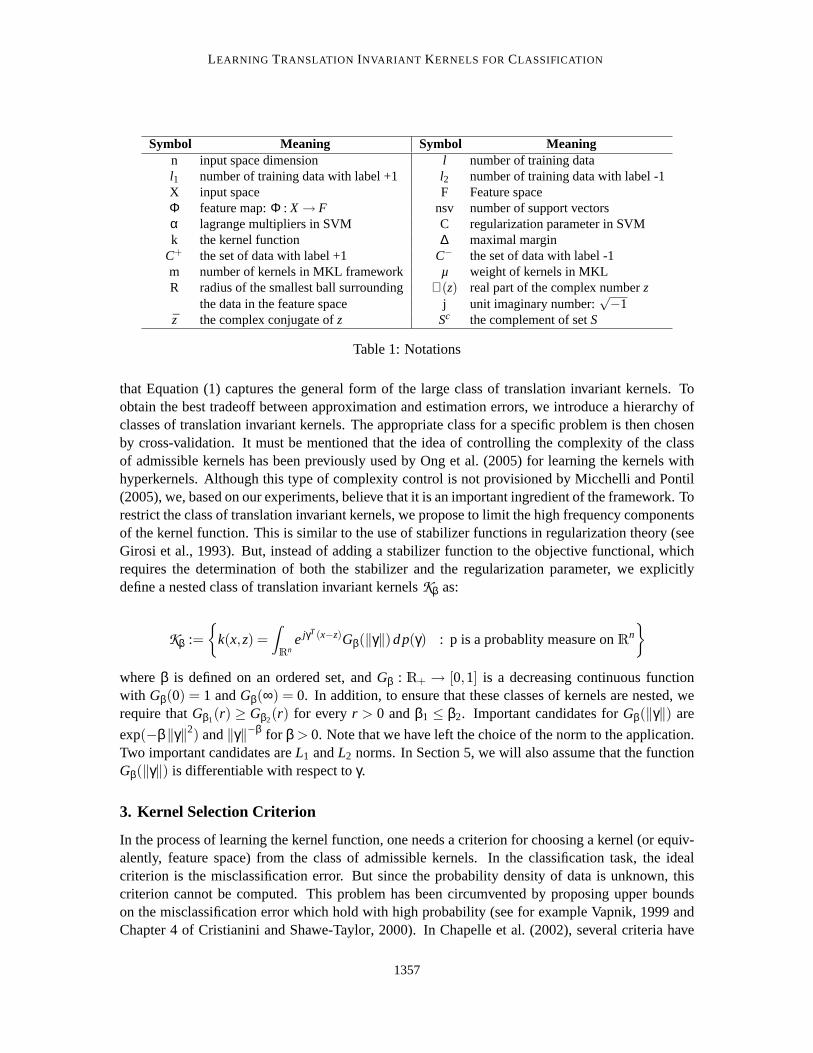
that Equation (1) captures the general form of the large class of translation invariant kernels. Toobtain the best tradeoff between approximation and estimation errors, we introduce a hierarchy ofclasses of translation invariant kernels. The appropriate class for a specific problem is then chosenby cross-validation. It must be mentioned that the idea of controlling the complexity of the classof admissible kernels has been previously used by Ong et al. (2005) forlearning the kernels withhyperkernels. Although this type of complexity control is not provisioned by Micchelli and Pontil(2005), we, based on our experiments, believe that it is an important ingredient of the framework. Torestrict the class of translation invariant kernels, we propose to limit the highfrequency componentsof the kernel function. This is similar to the use of stabilizer functions in regularization theory (seeGirosi et al., 1993). But, instead of adding a stabilizer function to the objective functional, whichrequires the determination of both the stabilizer and the regularization parameter, we explicitlydefine a nested class of translation invariant kernelsKβ as:
Kβ :=
k(x,z) =Z
RnejγT(x−z)Gβ(‖γ‖)dp(γ) : p is a probablity measure onRn
whereβ is defined on an ordered set, andGβ : R+ → [0,1] is a decreasing continuous functionwith Gβ(0) = 1 andGβ(∞) = 0. In addition, to ensure that these classes of kernels are nested, werequire thatGβ1(r) ≥ Gβ2(r) for every r > 0 andβ1 ≤ β2. Important candidates forGβ(‖γ‖) are
exp(−β‖γ‖2) and‖γ‖−β for β > 0. Note that we have left the choice of the norm to the application.Two important candidates areL1 andL2 norms. In Section 5, we will also assume that the functionGβ(‖γ‖) is differentiable with respect toγ.
3. Kernel Selection Criterion
In the process of learning the kernel function, one needs a criterion for choosing a kernel (or equiv-alently, feature space) from the class of admissible kernels. In the classification task, the idealcriterion is the misclassification error. But since the probability density of datais unknown, thiscriterion cannot be computed. This problem has been circumvented by proposing upper boundson the misclassification error which hold with high probability (see for example Vapnik, 1999 andChapter 4 of Cristianini and Shawe-Taylor, 2000). In Chapelle et al. (2002), several criteria have
1357

GHIASI-SHIRAZI , SAFABAKHSH AND SHAMSI
been studied and the authors suggested minimizing the radius-margin bound(R/∆)2 as the preferredcriterion.
Consider the training set of a classification task consisting of the input-output pairs(x1,y1), ...,(xl ,yl ), with yi ∈ −1,1. For a fixed kernel, support vector machines compute themaximal hard/soft margin separating hyperplane. By generalizing hard margin, 1-norm soft margin,and 2-norm soft-margin objective functions, Lanckriet et al. (2004) obtained the following general-ized criterion for 1/∆2 (which must be minimized):
ω′C′,τ′(k) := maxα : 0≤ α≤C′,
αTy = 0
2αTe−l
∑u=1
l
∑v=1
αuαvyuyvk(xu,xv)− τ′αTα
(2)
wheree is then×1 vector of ones and the prime sign is used to distinguish the parameters fromthose used in this paper. If(C′,τ′) is equal to(∞,0) ,(C′,0) , and (∞,1/C′), one obtains hardmargin, 1-norm soft margin, and 2-norm soft-margin performance measures, respectively. Our firstchange to this criterion is adding the constraintαTe = 2. It has been shown (Crisp and Burges,1999; Mavroforakis and Theodorodis, 2006) that by adjusting the parametersC and the offsetbappropriately, this new constraint does not change the separating hyperplane. However, the newconstraint plusαTy = 0 gives∑i∈C− αi = ∑i∈C+ αi = 1, which makes the exposition of our methodsimpler. Furthermore, we divide (2) by 1+ τ′ and defineτ := τ′
1+τ′ . So, in this paper we use thecriterion:
ωC,τ(k) := minα∈A
(1− τ)l
∑u=1
l
∑v=1
αuαvyuyvk(xu,xv)+ ταTα
(3)
whereA :=
α ∈Rl : 0≤ α≤C, αTy = 0, αTe= 2
. Note that in the new criterion max 1l1, 1
l2≤
C≤ 2 and 0≤ τ≤ 1. This criterion works well for a fixed kernel by maximizing the margin∆. Butin general, to minimize the radius-margin bound(R/∆)2, one must impose some constraint on theradius R, as well. For translation invariant kernels we haveR2 = ‖Φ(x)‖2 = k(x,x) = k(0). Hence,bounding the radiusR is equivalent to boundingk(0). One can easily verify that boundingtraceK,whereK is the kernel matrix in the transductive framework (see Lanckriet et al., 2004, Equation 17),also leads to a bound onk(0). Since by explodingR andtraceK, the margin∆ also explodes bythe same amount, whilst the radius-margin bound remains constant, we from now on assume thatk(0) = 1 and obtain the following optimization problem:2
supk
minα∈A
(1− τ)l
∑u=1
l
∑v=1
αuαvyuyvk(xu,xv)+ ταTα
s.t. k(x,z) =Z
RnejγT (x−z)Gβ(‖γ‖)dV(γ)
Z
RndV(γ) = 1,
V is monotonically increasing
2. Note that sincek is a complex-valued positive semi-definite kernel, the objective function isreal-valued and non-negative.
1358

LEARNING TRANSLATION INVARIANT KERNELS FORCLASSIFICATION
or equivalently
supp∈P (Rn)
minα∈A
Z
RnαTH(γ)α dp(γ) (4)
whereP (Γ) denotes the set of all probability measures onΓ andH(γ) is defined below. LetG(γ) bethel× l matrix whose(u,v)th entry isyuyvexp( jγT(xu−xv))Gβ(‖γ‖). DefineH(γ) := (1−τ)G(γ)+τIl whereIl is thel× l identity matrix. The following equation shows anO(l) computational methodfor computingαTG(γ)α:
αTG(γ)α =
∥
∥
∥
∥
∥
l
∑u=1
αuyuexp( jγTxu)
∥
∥
∥
∥
∥
2
2
Gβ(‖γ‖). (5)
4. Variational Optimization
In this section, we first prove the existence of a solution to problem (4). Next we prove that (4)can be written as a min-max problem with integration replaced by summation. This allows us tointroduce a SIP formulation of the problem. We then introduce another SIP problem for learningthe optimal kernel and parameterτ.
4.1 Replacing Sup with Max
We will prove that the sup operation in (4) can be substituted by the max operation. Note that all thevariability in the choice of a probability measurep from P (Rn) collapses to the choice of anl × lmatrix
R
Rn H(γ)dp(γ) from S(Cl ), whereS(Cl ) is the space of alll × l Hermitian complex-valuedmatrices. So, it is sufficient to prove that the set of all these matrices is compact, which ensuresthat any sequence of these matrices has a convergent subsequence,and subsequently, the supremumvalue is achieved. Furthermore, by compacting the parameter spaceA in (3) there is no need toassume that the kernel matrices are strictly positive definite, as was done in Lemma 2 of Micchelliand Pontil (2005).
LetC0(Rn) denote the function space of all continuous complex-valued functions defined onRn
which vanish at infinity, that is, lim‖γ‖→∞ g(γ) = 0 for anyg∈C0(Rn). By Theorem 3.17 of Rudin
(1987), the function spaceC0(Rn) with the norm
‖g‖ := maxγ∈Rn|g(γ)|
is a Banach space. Note that the use of max operation is justified by the continuity and vanish-ing properties ofg∈C0(R
n). Considering the above discussions, we need to prove the followingtheorem.
Theorem 1 For any fixed sample data Z= (x1,y1), ...,(xl ,yl ), the set
KZ :=
Z
RnH(γ)dp(γ) : p∈ P (Rn)
1359

GHIASI-SHIRAZI , SAFABAKHSH AND SHAMSI
is a compact subset of S(Cl ).3
Proof Consider any sequence(pn) in P (Rn). Define positive linear functionalsTn : C0(Rn)→ C
by Tng :=R
Rn g(γ)dpn(γ). So,Tn ∈C′0(Rn), the dual space ofC0(R
n). Since for eachn, ‖Tn‖= 1,by Banach-Alaoglu theorem (see for example Theorem 3.15 of Rudin, 1991 or page 237 of Royden,1988), there exists someT ∈C′0(R
n) with ‖T‖ ≤ 1 and a subsequence(Tm) such thatTm→ T inweak* topology. This means that for everyg∈C0(R
n), we haveTmg→ Tg. Since, each element ofthe matrixH(γ) belongs toC0(R
n), it follows thatR
Rn H(γ)dPm(γ)→ TH. One can easily prove bycontradiction that‖T‖= 1 andT is in fact a positive linear functional. By the Riesz representationtheorem (see Theorem 6.19 of Rudin, 1987), the functionalT can be represented uniquely by acomplex Borel measureµ ,with
R
Rn d|µ|= ‖T‖= 1, in the sense that
Tg=Z
Rngdµ for everyg∈C0(R
n).
The positivity ofT implies thatµ is a positive real measure. So,R
Rn dµ= 1 and consequentlyµis also a probability measure onRn. Thus,
Z
RnH(γ)dpm(γ)−→
Z
RnH(γ)dµ(γ)
which indicates that the setKZ is compact.
4.2 Interchanging themin and maxOperations
We first prove a theorem about interchanging the min and max operations which is an abstractedand generalized version of Theorem 20 in Micchelli and Pontil (2005).
Theorem 2 Assume thatΓ is a compact Hausdorff space and the function g: Γ×Rl → R is con-tinuous in the first parameter and convex and differentiable in the second parameter. LetE andIbe finite index sets , ai , where i∈ E ∪ I , be l×1 vectors, and bi , where i∈ E ∪ I , be real-valuedscalars. Considering problem (6), assume that the Slater’s condition (see Boyd and Vandenberghe,2004) holds, that is, there exists someα such that aTi α = bi for all i ∈ E and aT
i α < bi for all i ∈ I .Then there exist a discrete probability measurep∈ P (Γ) with at most l+1 atoms and some feasiblepoint α which solve the max-min problem
maxp∈P (Γ)
minα : aT
i α = bi for i ∈ E ,aT
i α≥ bi for i ∈ I
Z
Γg(γ,α)dp(γ) (6)
and the min-max problem
minα : aT
i α = bi for i ∈ E ,aT
i α≥ bi for i ∈ I
maxp∈P (Γ)
Z
Γg(γ,α)dp(γ) (7)
simultaneously. In addition, each atom ofp is a global maximum of g(γ, α) as a function ofγ.
3. Note that the topology ofS(Cl ) is the same as that ofRl2.An l × l hermitian matrix containsl real-valued diagonal
elements andl2−l2 independent complex-valued off-diagonal element.
1360

LEARNING TRANSLATION INVARIANT KERNELS FORCLASSIFICATION
Proof Assume thatα and p solve the problem (7). Define the function
φ : Rl →R
φ(α) := maxγ∈Γ g(γ,α)
and the set
Γ∗ := γ : γ ∈ Γ,g(γ, α) = φ(α) .
By Lemma 24 of Micchelli and Pontil (2005), the directional derivative ofφ along the directiond ∈Rl , denoted byφ′+(α;d), is given by:
φ′+(α;d) = max
γ∈Γ∗
dT∇αg(γ,α)
.
Sinceα minimizes (7), we have
φ′+(α;d) = max
γ∈Γ∗
dT∇αg(γ,α) |α=α
≥ 0 (8)
for any directiond such thataTi d = 0 for i ∈ E andaT
i d≥ 0 for i ∈ I ∗, whereI ∗ := i ∈ I : aTi α =
bi.Let M be the convex hull of the set of vectorsN := ∇αg(γ,α) |α=α : γ ∈ Γ∗ ⊆ Rl . Since
M ⊆ Rl , by the Caratheodory theorem (see for example Section 17 of Rockafellar, 1970) everyvector inM can be expressed as a convex combination of at mostl +1 elements ofN . We claimthat the set
O :=
∑i∈E∪I ∗
λiai : λi ≥ 0 for all i ∈ I ∗
intersectsM . Assume, on the contrary, thatM andO are distinct. SinceM is convex and compactandO is convex and closed, by the strict separating hyperplane theorem (seecorollary 11.4.2 ofRockafellar, 1970), there exists a separating hyperplanewTα+b = 0, w∈Rl , b∈R, such that
∑i∈E∪I ∗
λiwTai +b > 0, ∀λ : λi ≥ 0 for i ∈ I ∗
and
wT∇αg(γ,α) |α=α +b < 0, ∀γ ∈ Γ∗. (9)
The first condition, forλ = 0 implies thatb > 0 and sinceλi can take any real value fori ∈ Eand any nonnegative value fori ∈ I ∗, we have
1361

GHIASI-SHIRAZI , SAFABAKHSH AND SHAMSI
wTai = 0, ∀i ∈ E ,
wTai ≥ 0, ∀i ∈ I ∗.
By combining these results with (9), we get
maxγ∈Γ∗
wT∇αg(γ, α) |α=α < 0.
This means thatw is a feasible descent direction atα which contradicts (8). So, the setsO andM intersect. This means that there exist real numbersλi , i ∈ E , nonnegative numbersλi , i ∈ I ∗,and a discrete probability measure ˆp with at mostl +1 atoms such that
∑i∈E∪I ∗
λiai =Z
Γ∇αg(γ, α)dp. (10)
Now, we turn our attention to the solution of problem (6) forp = p. This is a convex opti-mization problem. Since by assumption the Slater’s condition holds, the KKT conditions provide anecessary and sufficient condition for optimality (see Boyd and Vandenberghe, 2004, page 244) andtherefore a solutionα to problem (6) is found by solving the following KKT conditions:
∑i∈E∪I
λiai =Z
Γ∇αg(γ, α)dp
aTi (α) = 0, i ∈ EaT
i (α)≥ 0, i ∈ Iλi ≥ 0, i ∈ I
λi(
aTi α−bi
)
= 0, i ∈ I .
By definingλi = 0 for i ∈ I \I ∗, using (10), and recalling the definition ofI ∗, it can be seen thatα, λ are the unique solution to the above KKT conditions. Thus,α = α and p = p solve problems(6) and (7) simultaneously and the theorem follows.
Corollary 3 Assume thatΓ is any compact subset ofRn and the parameter C is chosen4 suchthat C> max 1
l1, 1
l2. Then, there existα ∈ Rn and p ∈ P (Γ) that solve problems (11) and (12)
simultaneously. Furthermore,p is a discrete probability measure with at most l+1 atoms and eachatom ofp is a global maximum ofαTH(γ)α.
maxp∈P (Γ)
minα∈A
Z
ΓαTH(γ)α dp(γ), (11)
minα∈A
maxp∈P (Γ)
Z
ΓαTH(γ)α dp(γ). (12)
4. For a similar constraint in the context ofν-SVMs see Section 4 of Crisp and Burges (1999).
1362

LEARNING TRANSLATION INVARIANT KERNELS FORCLASSIFICATION
Proof It is sufficient to show that the Slater’s condition holds, that is, there existsα ∈Rl such thatαTe= 2, αTy = 0, α > 0, andα < C. One can easily verify that the choiceαi = 1
l1for i ∈C+ and
αi = 1l2
for i ∈C− satisfies these conditions.
In the rest of the paper, we assume thatC > max 1l1, 1
l2.
4.3 Confining Integration to a Compact Region
To write (4) as a min-max optimization problem, we first proved in Section 4.1 that the sup operationcan be replaced by the max operation. In the previous section we proved Corollary 3 which assertsthat if the integration region of (4) could have been replaced by a compactset, then the max andmin operations could also be interchanged. In this section, we show that the integration region of(4) can safely be confined to a compact subset ofRn. Let us first prove two useful lemmas.
Lemma 4 For arbitrary domains X and Y and every function f: X×Y→R, the following inequal-ity holds:
supx∈X
infy∈Y
f (x,y)≤ infy∈Y
supx∈X
f (x,y).
Proof Assume on the contrary that
supx∈X
infy∈Y
f (x,y) > infy∈Y
supx∈X
f (x,y).
Then, there exist ˜x∈ X andy∈Y such that
infy∈Y
f (x,y) > supx∈X
f (x, y)
which contradicts with the existence off (x, y).
Lemma 5 If τ < 1, then there exists some compact subsetΓβ ofRn, independent ofα, where allγ’sthat maximizeαTH(γ)α lie in it.5
Proof For eachα ∈Rl we have
maxγ∈Rn
αTH(γ)α = (1− τ)maxγ∈Rn
∥
∥
∥
∥
∥
l
∑u=1
αuyuexp( jγTxu)
∥
∥
∥
∥
∥
2
2
Gβ(‖γ‖)
+ ταTα. (13)
Let t(α) denote the maximum value of the term in the braces in the above equation. SinceGβis continuous andGβ(0) = 1, there is an open ball around zero inRn such thatGβ(‖γ‖) > 0. Thisfact plus the conditionαTe= 2, ensure that the coefficient of at least one of the exponential termsin (13) is nonzero. Hence, the term in the braces in (13), as a function ofγ, is never identically zeroand thust(α) > 0. For all values ofγ with Gβ(‖γ‖) < t
4 we have
5. Note that by (3), the choiceτ = 1 is unrealistic.
1363
GHIASI-SHIRAZI , SAFABAKHSH AND SHAMSI
αTH(γ)α− ταTα =
∥
∥
∥
∥
∥
l
∑u=1
αuyuexp( jγTxu)
∥
∥
∥
∥
∥
2
Gβ(‖γ‖)≤ 4Gβ(‖γ‖) < t(α)
and the lemma’s assertion follows fromlimr→∞G(r) = 0.
Theorem 6 There exists an optimal solution(α, p) to problem (4) which is also a solution to itwhen the integration domain is confined to the compact setΓβ.
Proof Let (α, p) be a solution to problems (6) and (7) withΓ replaced byΓβ. By Lemma 4 andCorollary 3, we have the following sequence of inequalities:
maxp∈P (Γβ)
minα∈A
Z
Γβ
αTH(γ)α dp(γ)≤
maxp∈P (Rn)
minα∈A
Z
RnαTH(γ)α dp(γ)≤
minα∈A
maxp∈P (Rn)
Z
RnαTH(γ)α dp(γ)≤
minα∈A
maxp∈P (Rn)
Z
Rnmaxγ∈Rn
αTH(γ)α dp(γ) =
minα∈A
maxγ∈Rn
αTH(γ)α =
minα∈A
maxp∈P (Γβ)
Z
Γβ
αTH(γ)α dp(γ).
However, the first and the last terms are equal by Corollary 3.
4.4 Semi-infinite Programming Formulation
We have not yet addressed the problem of how (12) is to be really solvedon a machine. In thissection, we reformulate (12) as a semi-infinite programming problem for whichmany algorithmshave been proposed (see Hettich and Kortanek, 1993; Reemtsen and Gorner, 1998, for two reviewson the subject).
Theorem 7 Let α and t be a solution to the semi-infinite programming problem (14) and define
the setΓHβ (α) :=
γ ∈ Γβ : αTH(γ)α = maxγ∈ΓβαTH(γ)α
. Let (Q) be the QCQP problem that is
obtained by replacingΓβ byΓHβ (α)≡ γ1, ...,γm in (14) and letµ1, ..., µm be a set of Lagrange mul-
tipliers associated with the constraints t≥ αTH(γi)α, 1≤ i ≤m which optimize the dual problemof (Q). If p is the discrete probability measure defined byp(γi) := µi i = 1, ...,m, thenα and p solvethe problem (4). In addition, there exists a solution pair(α∗, p∗) such thatp∗ contains at most l+1nonzero atoms.
1364
LEARNING TRANSLATION INVARIANT KERNELS FORCLASSIFICATION
minα,t t
s.t. t ≥ αTH(γ)α for all γ ∈ Γβ
0≤ α≤C
αTy = 0
αTe= 2.
(14)
Proof Since for allγ /∈ ΓHβ (α) the strict inequalityt > αTH(γ)α holds,α and t also solve the fol-
lowing QCQP problem:
minα,t t
s.t. t ≥ αTH(γi)α i = 1, ...,m
0≤ α≤C
αTy = 0
αTe= 2.
In addition, fromt = αTH(γ1)α = ... = αTH(γm)α, it follows thatα andt also solve the follow-ing problem:
minα∈A
maxµ≥0, ∑m
i=1 µi=1αT
[
m
∑i=1
µiH(γi)
]
α (15)
By Theorem 17 of Lanckriet et al. (2004), if ˜µ is chosen as specified by the statement of thistheorem, thenα andµ simultaneously solve the min-max problem (15) and the following max-minproblem:
maxµ≥0, ∑m
i=1 µi=1minα∈A
αT
[
m
∑i=1
µiH(γi)
]
α
which can also be written as
maxp∈P (ΓH
β (α))minα∈A
Z
αTH(γ)α dP(γ)
The first assertion of the theorem follows from the following inequalities:
t = maxp∈P (ΓH
β (α))minα∈A
Z
αTH(γ)α dP(γ)≤
maxp∈P (Γβ)
minα∈A
Z
αTH(γ)α dP(γ)≤
minα∈A
maxp∈P (Γβ)
Z
αTH(γ)α dP(γ) = t
1365
GHIASI-SHIRAZI , SAFABAKHSH AND SHAMSI
where the last equality follows from a simple reformulation of problem (14). The last part of thetheorem follows from Corollary 3 and reversing the above proof.
4.5 Including Other Kernels in the Learning Process
Although the focus of this paper is on the task of learning translation invariant kernels, it is easyto furnish the set of admissible kernels with other kernel functions. For example, one may want tofind the best convex combination of stabilized translation invariant kernels along with isotropic/non-isotropic Gaussian kernels, and polynomial kernels with degrees one to five.6 In general, assumethat we haveM classes of kernels
Ki :=
kγ(x,z) : γ ∈ Γi
i = 1, ...,M
whereΓ1, ...,ΓM are distinct compact Hausdorff spaces. Fori ∈ 1, ...,M let Gi(γ) be thel × l matrixwhose(u,v)’s entry isyuyvkγ(xu,xv) and defineHi(γ) := (1−τ)Gi(γ)+τIl . The problem of learningthe best convex combination of kernels from these classes for classification with support vectormachines can be stated as
supp∈P (Γ0)
minα∈A
Z
Γ0
αTH0(γ)α dp(γ) (16)
whereΓ0 := Γ1∪ ...∪ΓM and
H0(γ) :=
H1(γ) i f γ ∈ Γ1
H2(γ) i f γ ∈ Γ2...
HM(γ) i f γ ∈ ΓM
.
The results of the previous sections will hold for this combined class of kernels if we prove thatΓ0 is a compact Hausdoff space and thath0(γ,α) := αTH0(γ)α is continuous with respect toγ. LetTi denote the topology onΓi for i ∈ 1, ...,M. Define the setT0 of subsets ofΓ0 as:
T0 := O1∪O2...∪OM : O1 ∈ T1,O2 ∈ T2, ...,OM ∈ TM .
Proposition 8 T0 is a topology.
Proof ClearlyΓ0∈ T0. Next we must show thatT0 is closed under arbitrary union. LetO=S
i∈IOi
whereOi ∈ T0 andI is an arbitrary index set. We have
O =[
j∈1,...,M
(
[
i∈I
Oi ∩Γ j
)
6. Although the class of translation invariant kernels includes the set of isotropic/non-isotropic Gaussian kernels, it isnot the case for the stabilized classKβ.
1366

LEARNING TRANSLATION INVARIANT KERNELS FORCLASSIFICATION
which shows thatO∈ T0. Finally, we should show that finite intersection of closed sets is a closedset. Assume thatC =
Tri=1Ci , wherer ∈N andCc
i ∈ T0 . We have
Cc =[
i∈1,...,rCc
i =[
i∈1,...,r
[
j∈1,...,M(Cc
i ∩Γ j) .
SinceCci andΓ j are both open inT j , the setCc
i ∩Γ j is open inT j . By the properties of topologiesT1, ...,TM and the definition of topologyT0 it follows thatCc ∈ T0 which shows thatC is closed inT0.
Proposition 9 Assume that the functions hi(γ,α) : Γi ×Rl → R defined as hi(γ,α) = αTHi(γ)α,where i= 1, ...,M, are continuous in the first parameter. Then, the function h0(γ,α) : Γ0×Rl →R defined as h0(γ,α) = αTH(γ)α ,where the topology ofΓ0 is T0, is also continuous in the firstparameter.
Proof Fix α to any value and definehi(γ) := hi(γ,α) for i = 0, ...,M. Let O be an open subset ofR.We must show thath−1
0 (O) is open in topologyT0. We have
h−10 (O) =
[
i=1,...,M
(
h−10 (O)∩Γi
)
=[
i=1,..,M
h−1i (O).
Since the seth−1i (O) is open inTi for eachi ∈ 1, ...,M, it follows from the definition ofT0
that the union of these sets is also open inT0. So,h−10 (O) is open inT0 and the result follows.
Proposition 10 The setΓ0 with topologyT0 is compact in itself.
Proof Let O = Oi : i ∈ I0 be an open covering ofΓ0, whereI0 is some index set. Letj beany number in the set1, ...,M. SinceΓ j ⊆ Γ0, the setO is also an open covering forΓ j . Bycompactness ofΓ j , there exists a finite index setI j ⊆ I0 such that the set
Oi : i ∈ I j
is an opensubcovering ofΓ j . Thus, the setOi : i ∈ I1∪ ...∪ IM is a finite open subcovering ofT0 whichproves thatΓ0 is compact.
Proposition 11 Assume that topologiesT1, ...,TM are Hausdorff. Then, so is the topologyT0.
Proof We must prove that for any two pointsγ1,γ2 ∈ Γ0 there are disjoint open setsO1 andO2 suchthat γ1 ∈ O1 andγ2 ∈ O2. If γ1 andγ2 belong to the same setΓ j for some j ∈ 1, ...,M, then theassertion follows from the Hausdorffness property ofT j . Without loss of generality, assume thatγ1 ∈ Γ1 andγ2 ∈ Γ2. The choiceO1 = Γ1 andO2 = Γ2 completes the proof.
Theorem 12 Assume thatΓ1, ...,ΓM are compact Hausdorff spaces and the matrices Hj are asdefined previously in this section. Furthermore, assume that for j= 1, ...,M the functions hj(γ,α) :Γ j → Rl defined by hj(γ,α) := αTH j(γ)α are continuous in the first parameter. Letα and t be asolution to the semi-infinite programming problem P(Γ1, ...,ΓM), which is defined as
1367
GHIASI-SHIRAZI , SAFABAKHSH AND SHAMSI
minα,t t
s.t. t ≥ αTH1(γ)α for all γ ∈ Γ1
...
P(Γ1, ...,ΓM) := t ≥ αTHM(γ)α for all γ ∈ ΓM (17)
0≤ α≤C
αTy = 0
αTe= 2.
Define the setΓHj (α) :=
γ ∈ Γ j : αTH j(γ)α = maxγ∈Γ j αTH j(γ)α
. Let (Q) be the QCQP prob-
lem that is obtained by replacing everyΓ j with j = 1, ...,M by ΓHj (α) ≡
γ j1, ...,γ
jmj
in (17). For
any j∈ 1, ...,M let µj1, ..., µ
jmj be a set of Lagrange multipliers associated with the constraints
t ≥ αTH j(γji )α, 1≤ i ≤mj which optimize the dual problem of (Q). Ifp is the discrete probability
measure defined byp(γ ji ) := µj
i i = 1, ...,mj j = 1, ...,M, then the pair(α, p) solves the problem(16). In addition, there exists a solution pair(α∗, p∗) such thatp∗ contains at most l+ 1 nonzeroatoms.
Proof The result is immediately obtained by replacing the setΓβ by Γ0 in Theorem 7.
4.6 Automatic Adjustment of the Parameterτ
In this section, we consider the following problem:
max0≤τ≤1,p∈P (Rn)
minα∈A
Z
RnαTH(γ)α dP(γ). (18)
It is well known that the parameterτ can be envisioned as the weight of the kernelδ(x,z), whereδ is the Kronecker delta function. So, the problem of learning the parameterτ is equivalent tochoosing the best convex combination of the set of translation invariant kernels augmented with thedelta kernelδ(x,z). By using Theorem 12 we get the following corollary.
Corollary 13 Let α andt be a solution to the semi-infinite programming problem Pτ(Γβ), where foreach compact setΓ the problem Pτ(Γ) is defined by (19). Define the set
ΓGβ (α) :=
γ ∈ Γβ : αTG(γ)α = maxγ∈ΓβαTG(γ)α
.
Let (Q) be the QCQP problem that is obtained by replacingΓ byΓGβ (α)≡γ1, ...,γm in (19) and let
µ1, ..., µm be a set of Lagrange multipliers associated with the constraints t≥ αTG(γi)α, 1≤ i ≤mwhich optimize the dual problem of (Q). In addition, letµ0 be a Lagrange multiplier associated withthe constraint t≥ αTα in the dual problem of (Q). Ifp is the discrete probability measure definedby p(γi) := µi i = 1, ...,m andτ := µ0, thenα, τ, and p solve the problem (18). In addition, thereexist some solutionα∗, τ∗, and p∗ such thatp∗ contains at most l+1 nonzero atoms.
1368

LEARNING TRANSLATION INVARIANT KERNELS FORCLASSIFICATION
Pτ(Γ) :=
minα,t t
s.t. t ≥ αTG(γ)α for all γ ∈ Γt ≥ αTα0≤ α≤C
αTy = 0
αTe= 2.
(19)
Proof Let ω0 /∈ Γβ and assign the kernelδ(x,z) to this point. The corollary is proved by applyingtheorem 12 to the setsΓβ andω0.
4.7 Furnishing the Class of Admissible Kernels with Isotropic Gaussian Kernels
Although the class of translation invariant kernels encompasses the class of Gaussian kernels witharbitrary covariance matrices, the stabilized class of translation invariant kernelsKβ does not. So, itmay be advantageous to combine the classKβ with the class of Gaussian kernels. In this section, weconsider learning the best convex combination of kernels of the classesKβ and the stabilized classof isotropic Gaussian kernels
Kη :=
k(x,z) =Z
R
e−ω‖xu−xv‖2e−η‖ω‖2 dp(ω) : p is a probablity measure onR
whereη > 0. We also learn the parameterτ automatically. The proof that there exists some compactsetΩη ⊆ R where we can confine the integration to it parallels the discussion of Section 4.3 and isomitted. By using Theorem 12, it follows that the expansion of the optimal kernel along with theweight of each kernel can be obtained by solving the SIP problemPτ(Γβ,Ωη), wherePτ(Γ,Ω) isdefined as:
Pτ(Γ,Ω) :=
minα,t t
s.t. t ≥ αTG(γ)α for all γ ∈ Γ
t ≥l
∑u=1
l
∑v=1
αuαvyuyve−ω‖x−z‖2e−η‖ω‖2 for all ω ∈Ω
t ≥ αTα0≤ α≤C
αTy = 0
αTe= 2.
5. Optimization Algorithm
We now turn to the problem of numerically solving the nonlinear convex semi-infinite programmingproblemPτ(Γβ).7 The term semi-infinite stems from the fact that whilst the number of variables is
7. Modifying the proposed algorithm to solve problemPτ(Γ,Ω) is straightforward.
1369
GHIASI-SHIRAZI , SAFABAKHSH AND SHAMSI
finite, there is an infinite number of constraints which are indexed by the compact setΓβ. Hopefully,for each finite setΓ⊆Γβ, the problemPτ(Γ) is QCQP and therefore convex. Hence, in principle, onecan construct a sequence of QCQP problems with an increasing number ofconstraints such that theirsolutions converge to the solution of problemPτ(Γβ). This is the principle used by discretization andexchange algorithms (see Hettich and Kortanek, 1993; Reemtsen and Gorner, 1998). On the otherhand, by Corollary 13, only a finite number of constraints will be active in a solution. Furthermore,it is easy to show that this property is not limited to a solution point, and the active constraints at asolution also identify the active constraints in a neighborhood of it. This is the principle behind themethods based on local reduction (see Reemtsen and Gorner, 1998; Hettich and Kortanek, 1993).Reemtsen and Gorner (1998) proposed that to further speed up the methods based on local reduction,the set of active constraints be locally adapted. Combining these ideas with numerous experiments,we arrived at Algorithm 1. This algorithm is very similar to Algorithm 7 in Reemtsenand Gorner(1998) which is based on local reduction.
5.1 Choosing the Initial Value ofα
We choose the initial value ofα such that maximizing the criterion (3) with respect to the kernelfunction k and the parameterτ correspond to maximizing the distance of the means of the twoclasses in a feature space. Let us first write the distance between means of two classes in the featurespace of some kernelk′
‖m1−m2‖2 =
∥
∥
∥
∥
∥
1l1
∑u∈C+
Φ(xu)−1l2
∑v∈C−
Φ(xv)
∥
∥
∥
∥
∥
2
=1
l21
∑u∈C+
∑v∈C−
k′(xu,xv)+21
l1l2∑
u∈C+∑
v∈C−k′(xu,xv)+
1
l22
∑u∈C−
∑v∈C−
k′(xu,xv).
By choosingαi = 1/l1 for i ∈C+ andαi = 1/l2 for i ∈C−, we have
‖m1−m2‖2 =l
∑u=1
l
∑v=1
αuαvyuyvk′(xu,xv).
Comparing the above equation with (3), we see that maximizing the criterion (3) with respect tothe kernel functionk and the parameterτ is equivalent to maximizing the distance between meansof the samples of the two classes in the feature space of kernelk′(x,z) = k(x,z)+τδ(x,z). Note thatthis choice forα also satisfies the required conditionsαTe= 2, αTy = 0, and max 1
l1, 1
l2 ≤ α≤C;
and thusα ∈ A .
5.2 Global Search for Local Maxima ofαTG(γ)α
The algorithm presented in this section attempts to gather a subset of unsatisfied constraints to beconsidered in the next iteration of Algorithm 1. Although at the solution pointα the set of activeconstraints globally maximizeαTG(γ)α, for other choices ofα it is possible that the constraintsbe violated by the local maxima of the functionαTG(γ)α. So, in Algorithm 2, we try to find the
1370

LEARNING TRANSLATION INVARIANT KERNELS FORCLASSIFICATION
values ofγ which locally maximize the functionαTG(γ)α for givenα. Here we also assume that thefunctionGβ(‖γ‖) is differentiable with respect toγ. The choice of limited-memory BFGS algorithm(Nocedal, 1980; Liu and Nocedal, 1989; Nocedal and Wright, 2006) for this optimization is veryimportant. For large-scale problems with largen, the memory needed to store the Hessian matrixand the associated computations become prohibitive. Although a gradient-ascent algorithm doesnot compute the Hessian matrix, its convergence rate is very slow. The limited-memory BFGSalgorithm provides an excellent practical compromise between the computations at each step andthe number of iterations till convergence, without storing the full Hessian matrix in memory.
Algorithm 1 General Optimization AlgorithmRequire: T1
1. Γ(0)← , t(0)← 1l1
+ 1l2
A lower bound for parameter t is the minimum value ofαTα for α ∈ A2. Initialize α(0) as described in Section 5.13. for i = 1,2, ... do4. setR such that for allγ with ‖γ‖> R, the relationαTG(γ)α < t(i−1) holds for allα5. Γ(i)
g ←GlobalSearchForLocals(α(i−1),R)denote the maximum value obtained by the global search bys(i)
6. Γ(i)s ← Γ(i−1) S
Γ(i)g
7. Solve problemPτ(Γ(i)s ) to obtain the optimal parameterst(i)s ,α(i)
s andµ(i)s
see Section 5.38. Locally adaptΓ(i)
s andµ(i)s to obtain the optimal parameterst(i)l ,α(i)
l ,Γ(i)l andµ(i)
lsee Section 5.4
9. t(i)← t(i)l , α(i)← α(i)l
10. Constructµ(i) andΓ(i) by eliminating zero indices ofµ(i)l along with the corresponding vectors
in Γ(i)l
11. if t(i)− t(i−1) < εt(i−1) or i = T1 then12. terminate algorithm with the kernelk(x,z) := ∑m
j=1µ(i)j cos
(
(x−z)Tγ(i)j
)
we assume thatΓ(i) =
γ(i)1 , ...,γ(i)
m
and thatµ(i)j is the Lagrange multiplier associated
with the constraintαTG(γ(i)j )α≤ t in problemPτ(Γ(i))
13. end if14. end for
5.3 Solving the ProblemPτ(Γ) for Finite Set Γ
Let Γ = γ1, ...,γm be a finite subset ofΓβ. SinceΓ is finite, the problemPτ(Γ) can be written asthe following QCQP problem:
1371

GHIASI-SHIRAZI , SAFABAKHSH AND SHAMSI
Algorithm 2 GlobalSearchForLocalsRequire: α, R, T2, andT3
1. Γ = , i = 02. for j = 1,2, ... do3. generate a random pointx∈Rn
4. generate a random numberr ∈ [0,R]5. γ0← r x
‖x‖6. starting fromγ0 and using the limited-memory BFGS algorithm find a local maximumγ(i)
for functionαTG(γ)α7. if γ(i) ∈ Γ then8. i← i +1 count the number of repeating local maxima9. end if
10. Γ← Γ∪ γ(i)
11. if (i−|Γ|)≥ T2 or j = T3 then12. return Γ13. end if14. end for
minα,t t
s.t. t ≥ αTG(γi)α for all i = 1, ...,m
t ≥ αTα0≤ α≤C
αTy = 0
αTe= 2.
(20)
This problem has been studied in Section 4.6 of Lanckriet et al. (2004) and it has been suggestedto store thel × l kernel matricesG(γ1), ...,G(γm) in memory and solve the problem with generalpurpose software packages. But, the memory requirement of this approach limits its applicability tosmall-sized problems. However, the facts that
αTℑG(γ)α = 0
and
ℜG(γ)= vc(γ)Tvc(γ)+vs(γ)Tvs(γ),vc(γ) :=
[
y1cos(γTx1), y2cos(γTx2), . . . ,yl cos(γTxl )]
,
vs(γ) :=[
y1sin(γTx1), y2sin(γTx2), . . . ,yl sin(γTxl )]
1372
LEARNING TRANSLATION INVARIANT KERNELS FORCLASSIFICATION
whereℜz and ℑz are the real and imaginary parts ofz, respectively, show that the kernelmatricesG(γ1), ...,G(γm) appearing in problem (20) are effectively8 of rank two. This allows us toreformulate (20) as a new QCQP problem as follows:
minα,t,c,s t
s.t. t ≥ c2i +s2
i i = 1, ...,m
ci =l
∑u=1
αiyi cos(γTi xu) i = 1, ...,m
si =l
∑u=1
αiyi sin(γTi xu) i = 1, ...,m
t ≥ αTα0≤ α≤C
αTy = 0
αTe= 2.
(21)
Now, there is no need to load the kernel matrices into memory and so general-purpose QCQPsolvers such as Mosek (Andersen and Andersen, 2000) can be used to solve (21) even when thetraining set size is huge.
5.4 Local Adaptation
As stated in the previous section, for any finite setΓ = γ1, ...,γm⊆Γβ, the problemPτ(Γ) is convexand so every local solution is also globally optimal. But, if we consider the valuesγ1, ...,γm as pointsin the spaceRn, we get the following non-convex optimization problem:
maxµ≥ 0,µTe= 1,γ1, ...,γm∈Rn
minα∈A
m
∑i=1
µiαTG(γi)α+µ0αTα. (22)
Now, we can use the the solution of the problemPτ(Γ) obtained in the previous section as thestarting point for problem (22) and locally improve it by an ascent method. Byunrolling (22), weobtain the following optimization problem:
maxµ∈Rm+1,
γ1, ...,γm∈Rn
J(µ,γ1, ...,γm) s.t. µ≥ 0,µTe= 1 (23)
where
8. In this paper, we say that a matrixG is effectively of rankr if there exists some matrixH of rank r such that for allvectorsα ∈ A we haveαTGα = αTHα.
1373
GHIASI-SHIRAZI , SAFABAKHSH AND SHAMSI
J(µ,γ1, ...,γm) :=
minα∈A
l
∑u=1
l
∑v=1
αuαvyuyv
m
∑i=1
µiGβ (‖γi‖)cos(γTi (xu−xv))+µ0
l
∑u=1
α2u
. (24)
Problem (23), corresponds to adapting the kernel parametersγ1, ...,γm andµ0, ...,µm of the kernelfunction k(x,z) = ∑m
i=1µi cos(γTi (x−z)) + µ0δ(x− z) for the task of SVM classification, whereδ
denotes the Kronecker delta function. This problem has been previouslystudied by Chapelle et al.(2002) for general kernel functions with unconstrained parameters and they proved that the functionJ(.) is differentiable provided that problem (24) has a unique solution.9 They also proposed a simplegradient-based iterative algorithm for adapting the kernel parameters. Recently, Rakotomamonjyet al. (2008) performed a more detailed analysis of this problem in MKL and proposed a reducedgradient algorithm with line search. They reasoned that since the computationof the functionJ iscostly,10 the overhead of a line search preserves the effort.
To avoid the difficulties of the constrained optimization, we replace the constrained vectorµ by
the unconstrained vectorρ, connected by the relationµi =ρ2
iρT ρ , i = 0, ...m, and rewrite (23) as the
following problem:
maxρ ∈Rm+1,
γ1, ...,γm∈Rn
J(ρ,γ1, ...,γm) (25)
where
J(ρ,γ1, ...,γm) :=
minα∈A
1ρTρ
l
∑u=1
l
∑v=1
αuαvyuyv
m
∑i=1
ρ2i Gβ (‖γi‖)cos(γT
i (xu−xv))+ρ20
l
∑u=1
α2u
. (26)
We use the limited-memory BFGS algorithm to numerically solve (25). Our experiments onMKL tasks show that the method proposed in this section is several times fatserthan the reducedgradient algorithm of Rakotomamonjy et al. (2008).11 It has been also stated by Rakotomamonjyet al. (2008) that their method could be improved if the Hessian matrix could be computed ef-ficiently. This is not the case for the problem (25) withm× (n+ 1) variables; where, even formoderate size problems, the storage of the Hessian matrix requires lots of memory.
5.5 Solving the Intermediate SVM Problem and Its Gradient
To compute the functionJ(.) defined by Equation (26), we have to solve the following constrainedquadratic programming problem:
9. Truely speaking, the proof should be credited to Danskin (1966).10. Although the definition of the functionJ in Rakotomamonjy et al. (2008) differs from (24), computation of both
functions corresponds to training a single-kernel SVM.11. We leave this comparison along with some theoretical results to another paper.
1374
LEARNING TRANSLATION INVARIANT KERNELS FORCLASSIFICATION
minα αT
(
m
∑i=1
ρ2i
ρTρG(γi)
)
α+ρ2
0
ρTραTα
s.t. 0≤ α≤C
αTy = 0
αTe= 2.
(27)
Although the traditional algorithms for solving quadratic programming problems,such as activeset methods, are fast, they need to store the kernel matrix in memory which prevents their applicationin large-scale problems. So, various algorithms for large-scale training ofSVMs, such as SMO(Platt, 1999) orSVMLight (Joachims, 1999), have been proposed. Again, since the effective rank ofthe kernelsG(γ1), ...,G(γm) is two, we can re-state the problem (27) in a memory efficient manneras:
minα,c,sρ2
0
ρTραTα+
m
∑i=1
ρ2i
ρTρ(
c2i +s2
i
)
s.t. ci =l
∑u=1
αuyucos(γTi xu) i = 1, ...,m
si =l
∑u=1
αuyusin(γTi xu) i = 1, ...,m
0≤ α≤C
αTy = 0
αTe= 2.
In our experiments we have used the optimization software Mosek (Andersen and Andersen,2000) to solve this problem. After computing the value of the functionJ(.) and obtaining a solutionα to (26), we compute the gradient using the following formulas:
∇γ j J =ρ2
j
ρT ρ ∇γ
αTG(γ)α
|γ=γ j j = 1, ...,m, (28)
∇ρ j J = 2 ρ j
ρT ρ
αTG(γ j)α−∑mi=1
ρ2i
(ρT ρ)αTG(γi)α− ρ2
0(ρT ρ)
αT α
j = 1, ...,m. (29)
Note that, in general, the computational complexity of computing formulas (28) and (29) isO(m× n× nsv2) as was pointed out by Rakotomamonjy et al. (2008).12 The following formulasshow anO(m× (nsv+n)) method for computing the gradient of functionJ(.).
∇γ j J =ρ2
j
ρT ρ
(
c2j +s2
j
)
∇γGβ(‖γ‖)|γ=γ j +2ρ2
j
ρT ρ
(
s′jsj +c′jc j
)
Gβ(‖γ j‖) j = 1, ...,m,
∇ρ j J = 2 ρ j
ρT ρ
(c2j +s2
j )Gβ(‖γ j‖)−∑mi=1
ρ2i
ρT ρ(c2j +s2
j )Gβ(‖γ j‖)− ρ20
ρT ρ αT α
j = 1, ...,m
where
12. Note that in Rakotomamonjy et al. (2008) the functionJ(.) has onlym variables, while here the number of variablesis m× (n+1).
1375

GHIASI-SHIRAZI , SAFABAKHSH AND SHAMSI
c j =nsv
∑u=1
αuyucos(γTj xu) j = 1, ...,m,
sj =nsv
∑u=1
αuyusin(γTj xu) j = 1, ...,m,
c′j =−nsv
∑u=1
αuyuxusin(γTj xu) j = 1, ...,m,
s′j =nsv
∑u=1
αuyuxucos(γTj xu) j = 1, ...,m.
5.6 Convergence Analysis
In this section, we study the convergence properties of Algorithm 1. We hope the contents of thissection help the reader to get a better feeling of this algorithm. For any finite orinfinite setΓ, wedenote the solution of problemPτ(Γ) by S(Γ). Let us first prove a useful lemma.
Lemma 14 If the loop inside Algorithm 1 is executed for the i’th iteration, then S(Γ(i)l ) = S(Γ(i)).
In other words, removing the constraints where their associated Lagrange multipliers are zero, does
not change S(Γ(i)l ).
Proof Assume thatΓ(i)l = γ1, ...,γm. Without loss of generality, we assume thatΓ(i) = γ1, ...,γm′,
wherem′ < m. Denote the Lagrangian ofPτ(Γ(i)l ) byL(α, t,µ,λ), whereµ1, ...,µm are the Lagrange
multipliers associated with the constraintsαTG(γ1)α≤ t, ...,αTG(γm)α≤ t, respectively, andλ ∈ Λdenotes the Lagrange multipliers associated with all other constraints. SincePτ(Γ
(i)l ) is convex, by
the strong duality we have
S(Γ(i)l ) = max
µ≥0,λ∈Λminα,t
L(α, t,λ,µ) = L(α∗, t∗,λ∗,µ∗)
where it is assumed thatα∗, t∗,λ∗, andµ∗ are a solution to problemS(Γ(i)l ). Sinceµ∗m′+1, ...,µ
∗m are
zero, we also have
S(Γ(i)l ) = max
µ1≥0,...,µm′≥0,λ∈Λminα,t
L(α, t,λ,µ).
Since the strong duality also holds forPτ(Γ(i)), the last expression is equal toS(Γ(i)) and thelemma follows.
Now, we prove that for anyε > 0 the Algorithm 1 converges, even without limiting the maximumnumber of iterations.
Proposition 15 The sequence of numbers t(0), t(1), ... generated by Algorithm 1 is increasing andbounded.
1376
LEARNING TRANSLATION INVARIANT KERNELS FORCLASSIFICATION
Proof By steps 6 and 8 of Algorithm 1, it follows thatS(Γ(i−1))≤ S(Γ(i)s ) andS(Γ(i)
s )≤ S(Γ(i)l ). By
Lemma 14,S(Γ(i)l ) = S(Γ(i)). So,t(i−1) = S(Γ(i−1)) ≤ S(Γ(i)) = t(i). By Equation (5) and the fact
that αTe= 2, it follows thatαTα ≤ 4 andαTG(γ)α ≤ 4 for all choices ofα andγ; and thus, thesequence is bounded.
Defineg(α,γ) := αTG(γ)α . The following theorem is essentially Theorem 7.2 of Hettich andKortanek (1993), where its proof is reconstructed here for the sake of completeness.
Theorem 16 Assume that in every run of step 5 of Algorithm 1 at least one global maximizer of thefunction g(α(i−1),γ) is found and that the steps 10-13 of the algorithm are omitted (Note that thekey point is the omission of step 10). Letα be any accumulation point of the sequenceα(0),α(1), ...and assume that t(i)ր t . Then the pair(α, t) is a solution of Pτ(Γβ).
Proof First note that sinceα(i) ∈ A andA is compact, a point of accumulation for the sequenceα(0),α(1), ... always exists. Recall the definition ofΩβ from Section 4.6 and define the functiong(α)as:
g(α) := maxγ∈Ωβ
αTG(γ)α
For simplicity, assume thatα(i)→ α. Let (α∗, t∗) denote a solution of problemPτ(Γβ). Clearlyt ≤ t∗. If t = t∗ then the theorem is proved. Assume on the contrary thatt < t∗. Then, there existsγ ∈ Ωβ such thatt < g(α, γ) = g(α). But, sinceαT α ≤ t, it follows that γ ∈ Γβ. For i = 0,1, ...
chooseγ(i) ∈Ωβ such thatg(α(i),γ(i)) = g(α(i)). We have
g(α)− t =[
g(α(i))− t]
+[
g(α)−g(α(i))]
=[
g(α(i),γ(i))− t]
+[
g(α)−g(α(i))]
(30)
On the other hand, by omission of step 10 from Algorithm 1, all constraints ofthe previousiterations will continue to appear in the next iterations. Sinceg(α,γ) is continuous,α is a feasiblepoint for all problemsPτ(Γ(i)), wherei = 0,1, ...,∞. Therefore,
g(α,γ(i))≥ supj=1,...,∞
t( j) = t for all i = 0,1, ... (31)
Using (31) in (30) we obtain
g(α)− t =[
g(α(i),γ(i))− t]
+[
g(α)−g(α(i))]
≤[
g(α(i),γ(i))−g(α,γ(i))]
+[
g(α)−g(α(i))]
.(32)
By continuity ofg(., .), the right hand side of (32) tends to zero, which contradicts the assump-tion t < g(α).
1377

GHIASI-SHIRAZI , SAFABAKHSH AND SHAMSI
6. Generalizing the Kernel Trick to Complex-valued Kernels
Consider a machine learning algorithm designed for a real-valued Euclidean space. The kernel trickfor real-valued kernels states that if all geometric concepts of an algorithmare defined solely basedon the dot-product operation, then by replacing all of these dot-products by a kernel functionk, wearrive at a version of the very algorithm running in a feature space associated with kernelk. Forcomplex-valued kernels, the dot-product of any two vectors may be complex-valued which makesthe application of these kernels to machine learning algorithms more tricky. We now introducea generalization of the kernel trick for complex-valued kernels. Assume that k(x,z) is a complex-valued kernel. Then there exists at least one complex feature space, say F , and a mappingΦ : X→Fsuch thatk(x,z) = 〈Φ(x),Φ(z)〉F . Each axis in the complex feature spaceF can be substituted bytwo real-valued axes, one representing the real part and the other the imaginary part. Let us callthis real-valued spaceG. To use the kernel trick, we replace the complex feature spaceF with theequivalent real feature spaceG. Now, we show that the dot product between elements ofG can becomputed by the real-valued kernel functionℜk(x,z),13 whereℜz is the real part ofz.
Theorem 17 Let F be a complex Hilbert space of dimension N (possibly infinite) and G thecorre-sponding2N-dimensional Hilbert space obtained by representing real and imaginary parts of F inseparate real axes. Then〈x′,z′〉G = ℜ〈x,z〉F , where x′ is the2N-dimensional vector obtained byconcatenating real and imaginary parts of x.
Proof For finiteN we have
ℜ〈x,z〉F= ℜN
∑i=1
xi zi = ℜN
∑i=1
(xrei + jxim
i )(zrei − jzim
i )
=N
∑i=1
(xrei zre
i +ximi zim
i ) =2N
∑i=1
x′iz′i = 〈x′,z′〉G
If F is infinite dimensional, then it has an orthonormal basis (see Kreyszig, 1989p.168) andx andz can have at most countably many nonzero elements (see Kreyszig, 1989 p.165) which weindicate by index setI. So,
ℜ〈x,z〉F= ℜ ∑i∈I
xi zi = ℜ ∑i∈I
(xrei + jxim
i )(zrei − jzim
i )
= ∑i∈I
(xrei zre
i +ximi zim
i ) = ∑i∈I
x′iz′i = 〈x′,z′〉G.
After fully developing the paper based on the complex-valued form of translation invariant ker-nels, one of the reviewers introduced us to the real-valued form of thesekernels as was discovered byBochner (1955). He proved that every continuous real-valued translation invariant positive definitekernel inRn has the general form
13. The fact that real part of a complex kernel is a real kernel is not new (see Scholkopf and Smola, 2002 page 31). But,as far as we know, the relation between the corresponding Hilbert spaces, as stated in the theorem, is new.
1378
LEARNING TRANSLATION INVARIANT KERNELS FORCLASSIFICATION
k(x,z) = k(x−z) =Z
RncosγT(x−z)dV(γ).
It is interesting that after applying the appropriate kernel trick to both real-valued and complex-valued forms of translation invariant kernels, the optimal kernel is found tobe a mixture of cosines.
7. The Method at Runtime
One frequently denounced feature of SVMs is that the resulting classifierhas an expansion based onsupport vectors. Although support vectors are considered to be sparse in the training set, the result-ing classifier is usually slower than other competing methods such as neural networks (Scholkopfet al., 1998). In general, the computation of a support vector classifier requiresO(n×nsv) steps.The problem becomes more severe when the kernel function becomes a combination of several ker-nels, where the computational complexity of evaluating the classifier grows upto O(m×n×nsv).For some kernels, such as the Gaussian kernel with isotropic covariancematrix, the computationtime can be reduced toO((m+ n)× nsv). Our method has the eminent property that the result-ing classifier is not expanded based on support vectors at all. Considering the SVM classifierf (x) = ∑nsv
u=1 αuyuk(x,xu)+b, we have
f (x) =nsv
∑u=1
αuyuk(x,xu)+b =nsv
∑u=1
αuyu
(
m
∑i=1
µi cos(γTi (x−xu))Gβ(‖γi‖)
)
+b
=m
∑i=1
µiGβ(‖γi‖)nsv
∑u=1
αuyu(
cos(γTi x)cos(γT
i xu)+sin(γTi x)sin(γT
i xu))
+b
=m
∑i=1
µiGβ(‖γi‖)[(
nsv
∑u=1
αuyucos(γTi xu)
)
cos(γTi x)+
(
nsv
∑u=1
αuyusin(γTi xu)
)
sin(γTi x)
]
+b.
But ∑nsvu=1 αuyucos(γT
i xu) and ∑nsvu=1 αuyusin(γT
i xu) are constant values. So, the computationalcomplexity of evaluating the classifier of the proposed method isO(m× n). Note that the clas-sifier has an expansion based on the number of kernels, instead of support vectors. In addition,by Theorem 2, the number of kernels is limited tol + 1. Furthermore, since the deletion of non-support vector samples from the training set has no effect on the optimal classifier, it follows thatm≤ nsv+1. Although, theoretically, the number of kernels can reach the number of support vec-tors, our experiments show that the number of kernels is usually a fraction of the number of supportvectors.
8. A Learning Theory Perspective
A common feature between the class of radial kernels, considered by Micchelli and Pontil (2005),and the class of translation invariant kernels, considered here, is that the kernels of both classes
1379
GHIASI-SHIRAZI , SAFABAKHSH AND SHAMSI
have the property thatk(x,x) = 1 for everyx∈Rn.14 Micchelli et al. (2005b) used this feature alongwith a result from Yiming and Zhou (2007) to obtain a probably approximately correct (PAC) upperbound on the generalization error of their kernel learning framework over the class of radial kernelfunctions. They concluded that the regularization parameter of a single-kernel learning machineis sufficient for controlling the complexity of the class of radial kernels, rejecting the use of anauxiliary method for controlling the complexity of the class of radial kernels.
But, the situation for translation invariant kernels is completely different. It iswell-known thatthe VC-dimension of the class of cosine functions with arbitrary frequencies is infinite (see Vapnik,1998, page 160). In addition, the finiteness of the VC-dimension is a necessary and sufficient condi-tion for distribution independent learning of binary classification tasks (see Vapnik, 1998, Theorem4.5). So, controlling the complexity of the class of translation invariant kernels is a necessary ingre-dient of our framework. This discussion will be experimentally verified in Section 9, where we willshow the vital role of the complexity control mechanism of Section 2.
9. Experimental Results
In this section we report the results of our experiments on several artificial and real-world bench-mark data sets. In addition, we will experimentally investigate the role of the complexity controlmechanism of Section 2. In all the experiments we have setC = ∞, T1 = 1000,T2 = 4, T3 = 500,Gβ(‖γ‖2) = exp(−β‖γ‖22)) and the parameterτ is automatically learnt according to Algorithm 1.The implementation of this paper is packaged in the SIKL (Stabilized infinite kernel learning) tool-box and is available athttp://www.mloss.org. We obtained the implementation of the limited mem-ory BFGS algorithm from the websitehttp://www.chokkan.org/software/liblbfgswhich is a C++translation of the original implementation made available by Nocedal in Fortran 77. For limited-memory BFGS algorithm, the 17 most recent curvature information are used and the maximumnumber of line-search tries is set to 20. We also changed the stopping condition of the algorithmfrom ‖∇x‖
‖x‖ < ε to ‖∇x‖ < ε to avoid the degradation of the accuracy of the global search algorithmfor points far from the origin. The QCQP sub-problem of Algorithm 1 and the QP problem ofSection 5.5 are solved by the optimization software Mosek (Andersen and Andersen, 2000). Allthe experiments have been performed on a 2.8GHz Pentium D computer with 2GBmemory andrunning the Linux operating system.
9.1 Experiments on Small-size Benchmark Data Sets
In this section, we report our experiments on the benchmark data sets prepared by Ratsch et al.(2001). This benchmark consists of 13 data sets and there exist 100 splitsof each data set intotraining and test sets. The classification error for each data set is obtained by averaging the classifi-cation error over these splits. For this experiment we setε = 0.001. The comparison is among thefollowing methods:
• Single Gaussian (SG)Ratsch et al. (2001) performed experiments with a single isotropicGaussian kernel. The variance parameterσ of the isotropic Gaussian kernel and the parameterC of the 1-norm soft-margin SVM are optimized by performing 5-fold cross-validation on thefirst five instances of the training set.
14. In fact, the classes of radial/translation invariant kernel functions contain kernels with arbitrary positive values fork(x,x). But, the constraintk(x,x) = 1 is imposed for reasons stated in Section 3.
1380

LEARNING TRANSLATION INVARIANT KERNELS FORCLASSIFICATION
• Gaussian Mixture (GM) A generalization of the method of Gehler and Nowozin (2008)is implemented and used for learning the optimal kernel over the classKη. The numberof Gaussian kernels ¯m, their parameters, and the parameterτ are learnt automatically. Theparameterη is set to 0.001 and the parameterC is learnt by performing 5-fold cross validationon the first five instances of the training set.
• Cosine Mixture (CM) Here, the method of Section 4.6 is used. The number of cosine kernelsm, their parameters, and the parameterτ are learnt automatically. The parameterC is fixedto ∞ and the parameterβ is optimized by performing 5-fold cross validation on the first fiveinstances of the training set.
• Cosine and Gaussian Mixture (CGM)Here, the method of Section 4.7 is used. The numberof cosine kernelsm, the number of Gaussian kernels ¯m, the parameters of cosine and Gaussiankernels, and the parameterτ are learnt automatically. The parameterC is set to∞ and theparameterη is set to 0.03. The parameterβ is optimized by performing 5-fold cross validationon the first five instances of the training set.
To compare the training and evaluation times of these methods, we repeated the experiments ofRatsch et al. (2001) on our machine. For training a single-kernel SVM we used the implementationof SMO algorithm (Platt, 1999) contained in the Statistical Pattern Recognition Toolbox.15 To keepthe results reported by Ratsch et al. (2001) as reference, we neglect the accuracies obtainedby theSG method.
Table 2 summarizes the test error rates and training times of the methods on each data set. It canbe seen that the GM method has the worst performance and does not provide any improvement overother methods. The only benefit of the GM over SG is that while the latter requires specifying thekernel function by hand, GM learns the kernel function automatically. TheSG and CM are the onlymethods of this experiment that do not store the kernel matrices in memory; andthus are applicableto large-scale problems. In addition, they have also the best training times. Toour surprise, althoughthe CM method solves a musch more difficult problem than SG, it has also improved the trainingtime in some data sets. Considering the test error rates, the CGM method has the best overallperformance. But, the SG method on theF.Solardata set, and CM method on theThyroiddata setprovide significantly better results. For theRingnormdata set, the CM method has obtained a higherror rate of 8.5%. Interestingly, the number of training and testing samples of theRingnormdataset are exactly equal to theTwonormdata set, for which the CM method has even improved theaccuracy. The essential difference between theTwonormand theRingnormdata sets, where in bothdata sets each class has a multivariate normal distribution, is that in theTwonormdata set the classeshave separate means, whilst in theRingnormdata set the classes have separate covariance matrices.So, it seems that the Gaussian kernel is inherently much more suitable for solving theRingnormdata set than the cosine kernel. In fact, this is exactly why combining several kernels is important.By combining the cosine and Gaussian kernels, the CGM method provides the best performance.
Table 3 compares the methods in terms of the evaluation time. For each method, the factors thatinfluence the evaluation time are also reported. As can be seen, except for theRingnormdata set,the CM is significantly faster at run-time than all other methods, including a classical SVM withGaussian kernel. The best speedup is for theTwonormdata set for which, in addition to a lower test
15. Available athttp://cmp.felk.cvut.cz/cmp/software/stprtool.
1381

GHIASI-SHIRAZI , SAFABAKHSH AND SHAMSI
Data SetSingle
GaussianGaussianMixture
CosineMixture
Cosine&GaussianMixture
error(%)
training(sec)
error(%)
training(sec)
error(%)
training(sec)
error(%)
training(sec)
Banana 11.5±0.7 1.1 10.5±0.5 26.4 10.7±0.5 3.5 10.4±0.5 21.3B. Cancer 26.0±4.7 0.2 26.7±5.0 2.7 26.2±4.9 1.2 25.8±4.7 4.2Diabetis 23.5±1.7 1.6 23.7±1.7 7.5 23.2±1.9 2.3 23.2±1.8 16.5F. Solar 32.4±1.8 9.1 35.4±1.7 15.4 33.3±1.8 1.2 33.9±1.8 57.7German 23.6±2.1 4.4 25.3±2.5 35.4 24.1±2.2 3.5 23.7±2.2 53.9Heart 16.0±3.3 0.1 17.0±3.2 1.4 15.6±3.2 1.1 16.0±3.2 2.8Image 3.0±0.6 16.0 3.6±1.3 178.9 2.5±0.5 1057.1 2.5±0.5 779.6Ringnorm 1.7±0.1 2.9 1.7±0.1 9.7 8.5±0.9 192.7 1.7±0.1 17.7Splice 10.9±0.7 445.4 11.1±0.7 91.8 9.7±0.4 43.3 9.3±0.5 187.0Thyroid 4.8±2.2 0.1 4.6±2.2 1.8 3.7±2.2 3.4 4.8±2.1 3.1Titanic 22.4±1.0 0.1 23.2±1.3 1.0 22.9±1.2 0.9 22.9±1.2 2.6Twonorm 3.0±0.2 0.4 2.7±0.2 7.9 2.4±0.1 5.4 2.7±0.2 17.9Waveform 9.9±0.4 5.8 9.8±0.4 8.5 10.0±0.5 2.6 9.7±0.4 17.7
Table 2: Test errors and training times of SG, GM, CM, and CGM methods on thedata sets col-lected by Ratsch et al. (2001)
Data SetSingle
GaussianGaussianMixture
CosineMixture
Cosine &Gaussian Mixture
testing nsv testing nsv m testing m testing nsv m m(ms) (ms) Gauss (ms) cos (ms) cos Gauss
Banana 144.7 153.1 615.9 375.7 2.1 13.4 13.6 611.3 393.1 2.0 2.5B. Cancer 2.2 122.3 4.8 200.0 1.8 0.4 3.6 0.5 200.0 4.3 0.1Diabetis 19.9 263.3 47.6 464.8 2.1 0.8 7.0 3.8 466.2 5.8 0.2F. Solar 49.9 507.9 354.0 666.0 1.6 0.6 2.1 1.3 666 11.0 0.0German 31.4 426.0 120.7 696.4 2.9 1.0 6.6 76.3 700.0 11.6 1.8Heart 2.2 84.3 6.4 163.1 1.9 0.3 1.8 5.1 169.8 1.6 1.5Image 205.4 700.7 765.1 1030.4 4.4 56.6 160.2 503.2 712.7 65.2 3.8Ringnorm 120.2 64.4 487.0 156.2 1.9 228.5 91.7 610.8 200.2 0.0 2.0Splice 357.7 385.4 1647.7 879.5 2.3 51.4 30.8 1293.6 755.7 13.5 1.6Thyroid 0.5 22.0 3.1 84.3 3.0 0.4 6.4 3.1 112.0 1.0 2.1Titanic 35.9 89.5 78.5 150.0 1.5 1.5 2.5 14.8 150.0 2.5 0.3Twonorm 332.6 167.4 455.7 180.6 1.5 3.5 1.0 582.1 226.2 0.0 1.5Waveform 134.3 104.5 587.4 290.5 1.9 6.0 2.9 731.9 374.7 1.0 1.6
Table 3: Experimentally measured evaluation times along with the parameters that theoretically de-termine the evaluation times of SG, GM, CM, and CGM methods on the data sets collectedby Ratsch et al. (2001)
error rate, the evaluation of the CM method is 95 times faster than a classical SVM with Gaussiankernel. This speedup in the evaluation of the classifiers can be very useful for applications targetedat small computers with limited computational power.
1382
LEARNING TRANSLATION INVARIANT KERNELS FORCLASSIFICATION
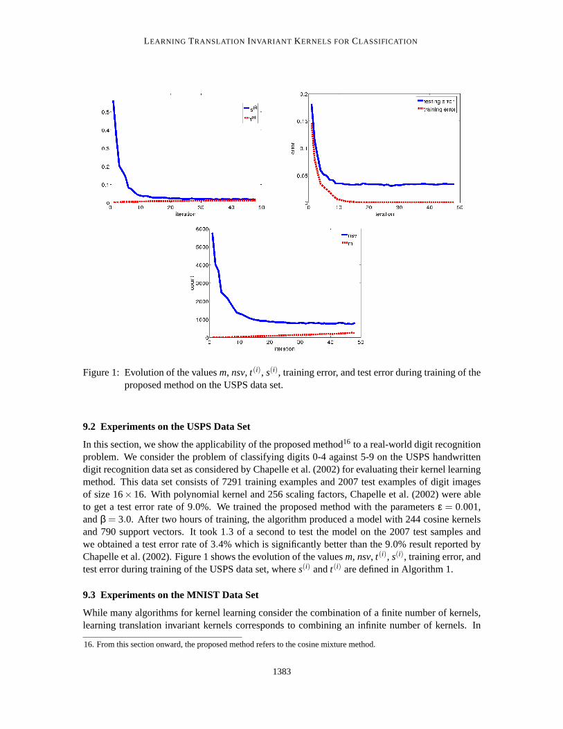
Figure 1: Evolution of the valuesm, nsv, t(i), s(i), training error, and test error during training of theproposed method on the USPS data set.
9.2 Experiments on the USPS Data Set
In this section, we show the applicability of the proposed method16 to a real-world digit recognitionproblem. We consider the problem of classifying digits 0-4 against 5-9 on the USPS handwrittendigit recognition data set as considered by Chapelle et al. (2002) for evaluating their kernel learningmethod. This data set consists of 7291 training examples and 2007 test examples of digit imagesof size 16×16. With polynomial kernel and 256 scaling factors, Chapelle et al. (2002) were ableto get a test error rate of 9.0%. We trained the proposed method with the parametersε = 0.001,andβ = 3.0. After two hours of training, the algorithm produced a model with 244 cosine kernelsand 790 support vectors. It took 1.3 of a second to test the model on the 2007 test samples andwe obtained a test error rate of 3.4% which is significantly better than the 9.0% result reported byChapelle et al. (2002). Figure 1 shows the evolution of the valuesm, nsv, t(i), s(i), training error, andtest error during training of the USPS data set, wheres(i) andt(i) are defined in Algorithm 1.
9.3 Experiments on the MNIST Data Set
While many algorithms for kernel learning consider the combination of a finite number of kernels,learning translation invariant kernels corresponds to combining an infinite number of kernels. In
16. From this section onward, the proposed method refers to the cosine mixture method.
1383

GHIASI-SHIRAZI , SAFABAKHSH AND SHAMSI
this section, we compare the proposed algorithm with the DC method proposed by Argyriou et al.(2006) which is based on the theory developed by Micchelli and Pontil (2005). They considered theproblem of finding an optimal kernel over the whole class of radial kernels which is equivalent tothe problem of learning the best convex combination of Gaussian kernels with isotropic covariancematrices.
Argyriou et al. (2006) performed a series of experiments on the MNIST data set by using thefirst 500 training examples for training and the first 1000 test examples forevaluation. The MNISTdata set contains 28×28 images of handwritten digits which are divided into 60,000 training and10,000 test examples. In addition, the results reported by the DC method have been obtained bysplitting each image into four sub-images which is a use of extra information. In the first exper-iment, we use the first 3,000 training examples17 for training both systems and evaluate them onthe whole test set. As Argyriou et al. (2006), we consider the tasks of classifying digits 3 vs.8, 4 vs. 7, and odds vs. evens. We downloaded the implementation of the DC method fromhttp://www.cs.ucl.ac.uk/staff/a.argyriou/code/dcand chose the range[75,25000] for the parameterσ of the Gaussian kernel which is the largest range considered by Argyriou et al. (2006). The pa-rameterµ of the DC method and the parameterβ of the CM method were optimized by hand. Theparameterε was set to the value 0.001. The first three rows of Table 4 show the results of thisexperiment. It can be seen that the main benefit of the DC method is its short training time, whilethe CM method has superiority in terms of the evaluation time.
Another remarkable feature of the CM method is its applicability to large-scale problems. Toillustrate this fact, we increased the size of the training set of the previous experiments from 3,000to 10,000. We also increased the parameterε from 0.001 to 0.01 to decrease the training time. TheDC method could not handle this size of training samples and ran out of memory.The last threerows and columns of Table 4 show the results of the experiments with the CM method. Figure 2depicts the evolution of the valuesm, nsv, t(i), s(i), training error, and test error during training ofCM algorithm on the ods vs even task with 10,000 training samples. Note that the model producedby the CM method on the larger training set is more accurate and faster-to-evaluate than the bestmodel that the DC algorithm could produce. We think that the capabilities of the CM method andDC method are complementary. The DC method works with full-rank matrices, is not large-scale,converges fast, and its model takes more time to compute. On the other hand, theCM method workswith low-rank matrices, is large-scale, converges slowly, and its model canbe evaluated very fast.One open problem is that whether these methods can be combined in a way thatthe benefits of bothmethods are achieved.
9.4 Assessing the Effect of the Proposed Complexity Control Mechanism
In Section 8 we provided theoretical support for the necessity of controlling the complexity of theclass of translation invariant kernels. Here we support this claim by experimenting on theHeartdata set chosen from the benchmark produced by Ratsch et al. (2001). This data set contains 170train patterns and 100 test patterns of dimension 13. The experiments of the previous section showthat the proposed method was completely successful in obtaining a low test error rate on this dataset. In addition, the mean error rate of the proposed method on the train set is14.0% which is closeto the mean error rate of 15.5% obtained on the test set. The left plot of Figure 3 illustrates thetrajectories of the train and test errors of the proposed method during training on theHeart data set.
17. This is approximately the largest possible train-set size where the DC method did not ran out of memory.
1384
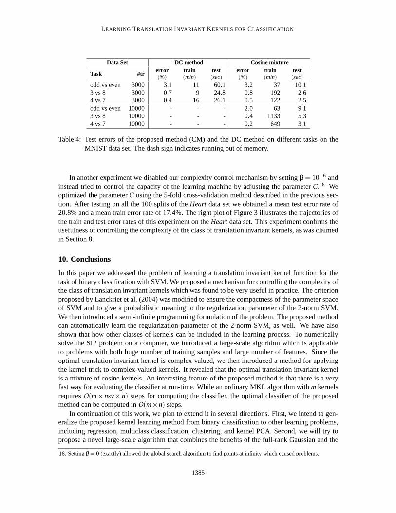
LEARNING TRANSLATION INVARIANT KERNELS FORCLASSIFICATION
Data Set DC method Cosine mixture
Task #trerror(%)
train(min)
test(sec)
error(%)
train(min)
test(sec)
odd vs even 3000 3.1 11 60.1 3.2 37 10.13 vs 8 3000 0.7 9 24.8 0.8 192 2.64 vs 7 3000 0.4 16 26.1 0.5 122 2.5odd vs even 10000 - - - 2.0 63 9.13 vs 8 10000 - - - 0.4 1133 5.34 vs 7 10000 - - - 0.2 649 3.1
Table 4: Test errors of the proposed method (CM) and the DC method on different tasks on theMNIST data set. The dash sign indicates running out of memory.
In another experiment we disabled our complexity control mechanism by setting β = 10−6 andinstead tried to control the capacity of the learning machine by adjusting the parameterC.18 Weoptimized the parameterC using the 5-fold cross-validation method described in the previous sec-tion. After testing on all the 100 splits of theHeart data set we obtained a mean test error rate of20.8% and a mean train error rate of 17.4%. The right plot of Figure 3 illustrates the trajectories ofthe train and test error rates of this experiment on theHeart data set. This experiment confirms theusefulness of controlling the complexity of the class of translation invariant kernels, as was claimedin Section 8.
10. Conclusions
In this paper we addressed the problem of learning a translation invariantkernel function for thetask of binary classification with SVM. We proposed a mechanism for controlling the complexity ofthe class of translation invariant kernels which was found to be very useful in practice. The criterionproposed by Lanckriet et al. (2004) was modified to ensure the compactness of the parameter spaceof SVM and to give a probabilistic meaning to the regularization parameter of the2-norm SVM.We then introduced a semi-infinite programming formulation of the problem. The proposed methodcan automatically learn the regularization parameter of the 2-norm SVM, as well. We have alsoshown that how other classes of kernels can be included in the learning process. To numericallysolve the SIP problem on a computer, we introduced a large-scale algorithmwhich is applicableto problems with both huge number of training samples and large number of features. Since theoptimal translation invariant kernel is complex-valued, we then introduced amethod for applyingthe kernel trick to complex-valued kernels. It revealed that the optimal translation invariant kernelis a mixture of cosine kernels. An interesting feature of the proposed methodis that there is a veryfast way for evaluating the classifier at run-time. While an ordinary MKL algorithm withmkernelsrequiresO(m× nsv× n) steps for computing the classifier, the optimal classifier of the proposedmethod can be computed inO(m×n) steps.
In continuation of this work, we plan to extend it in several directions. First,we intend to gen-eralize the proposed kernel learning method from binary classification to other learning problems,including regression, multiclass classification, clustering, and kernel PCA. Second, we will try topropose a novel large-scale algorithm that combines the benefits of the full-rank Gaussian and the
18. Settingβ = 0 (exactly) allowed the global search algorithm to find points at infinity which caused problems.
1385

GHIASI-SHIRAZI , SAFABAKHSH AND SHAMSI
Figure 2: Evolution of the valuesm, nsv, t(i), s(i), training error, and testing error during training ofthe proposed method with the first 10,000 samples of the MNIST data set for the task ofclassifying odds vs. evens.
Figure 3: Comparison between the parametersβ andC for controlling the capacity of the class oftranslation invariant kernels on theHeart data set.
1386
LEARNING TRANSLATION INVARIANT KERNELS FORCLASSIFICATION
low-rank cosine kernels. Third, we intend to investigate the applicability of theidea of Xu et al.(2008) about adding a regularization term that smoothes the fluctuating behaviour of SILP algo-rithms, to the proposed SIP algorithm. We hope that this study would greatly decrease the trainingtime of the proposed method. Another direction is to support the complexity control mechanismof Section 2 by introducing upper bounds for the generalization error ofthe proposed method. Ourlong time plan is to investigate the use of other low-rank kernels and make it a competing populartechnology.
Acknowledgments
The first author would like to thank professor Abdolhamid Riazi for allowinghim to participate inhis functional analysis class and helping him to get acquainted with the concepts of this graduatecourse. We also want to thank Stephen Boyd, Andreas Argoriou, and Peter Gehler for providing uswith their valuable materials.
References
S. Amari and S. Wu. Improving support vector machine classifiers by modifying kernel functions.Neural Networks, 12(6):783–789, 1999.
E.D. Andersen and K.D. Andersen. The MOSEK interior point optimizer forlinear programming:an implementation of the homogeneous algorithm. In T. Terlaky H. Frenk, K. Roos and S. Zhang,editors,High Performance Optimization, pages 197–232. Kluwer Academic Publishers, 2000.
A. Argyriou, C.A. Micchelli, and M. Pontil. Learning convex combinations ofcontinuously param-eterized basic kernels. InProceedings of the 18th Conference on Learning Theory, volume 18,pages 338–352, 2005.
A. Argyriou, R. Hauser, C.A. Micchelli, and M. Pontil. A DC-programming algorithm for kernelselection. InProceedings of the23rd International Conference on Machine Learning, volume 23,pages 338–352, Pittsburgh, PA, 2006.
F.R. Bach, G.R.G. Lanckriet, and M.I. Jordan. Multiple kernel learning, conic duality, and the SMOalgorithm. InProceedings of the 21st International Conference on Machine Learning, volume 21,pages 41–48, Banff, Canada, 2004. Omnipress.
S. Bochner. Monotone functions, Stieltjessche integrale und harmonischeanalyse.MathematischeAnnalen, 108:378–410, 1933.
S. Bochner.Harmonic Analysis and the Theory of Probability. University of California Press, LosAngeles, California, 1955.
S. Boyd and L. Vandenberghe.Convex Optimization. Cambridge University Press, Cambridge, UK,2004.
O. Chapelle, V. Vapnik, O. Bousquet, and S. Mukherjee. Choosing multipleparameters for supportvector machines.Machine Learning, 46(1-3):131–159, 2002.
1387
GHIASI-SHIRAZI , SAFABAKHSH AND SHAMSI
D.J. Crisp and C.J.C. Burges. A geometric interpretation ofν-svm classifiers. InAdvances in NeuralInformation Processing Systems, volume 12, pages 244–250, Cambridge, MA:, 1999. MIT Press.
N. Cristianini and J. Shawe-Taylor.An Introduction to Support Vector Machines. Cambridge Uni-versity Press, 2000.
Nello Cristianini, Colin Campbell, and John Shawe-taylor. Dynamically adapting kernels in supportvector machines. InAdvances in Neural Information Processing Systems 11, pages 204–210. MITPress, 1998.
F. Cucker and D.X. Zhou.Learning Theory: An Approximation Theory Viewpoint. CambridgeUniversity Press, Cambridge, UK, 2007.
J. M. Danskin. The theory of max-min, with applications.SIAM Journal on Applied Mathematics,14(4):641–664, 1966.
P. V. Gehler and S. Nowozin. Infinite kernel learning. InProceedings of the NIPS 2008 Workshopon ”Kernel Learning: Automatic Selection of Optimal Kernels”, pages 1–4, 2008.
M.G. Genton. Classes of kernels for machine learning: A statistics perspective. Journal of MachineLearning Research, 2:299–312, 2001.
F. Girosi, M. Jones, and T. Poggio. Priors, stabilizers and basis functions: from regularizationto radial, tensor and additive splines. A.I. Memo 1430, Artificial IntelligenceLabratory, Mas-sachusetts Institute of Technology, June 1993.
T. Glasmachers and C. Igel. Gradient-based adaptation of general Gaussian kernels.Neural Com-putation, 17:2099–2105, 2005.
R. Hettich and K.O. Kortanek. Semi-infinite programming: theory, methods, andapplications.SIAM Review, 35(3):380–429, 1993.
T. Joachims. Making large-scale support vector machine learning practical. In B. Scholkopf, C.J.C.Burges, and A.J. Smola, editors,Advances in Kernel Methods- Support Vector Learning, pages169–184. MIT Press, 1999.
E. Kreyszig.Introductory Functional Analysis with Applications. Wiley, New York, 1989.
G.R.G. Lanckriet, N. Cristianini, P. Bartlett, L. El Ghaoui, and M.I. Jordan.Learning the kernelmatrix with semidefinite programming.Journal of Machine Learning Research, 5:27–72, 2004.
D.C. Liu and J. Nocedal. On the limited memory BFGS method for large scale optimization. Math-ematical Programming B, 45(3):503–528, 1989.
M.E. Mavroforakis and S. Theodorodis. A geometric approach to support vector machine (SVM)classification.IEEE Transactions on Neural Networks, 17(3):671–682, 2006.
C.A. Micchelli and M. Pontil. Learning the kernel function via regularization. Journal of MachineLearning Research, 6:1099–1125, 2005.
1388
LEARNING TRANSLATION INVARIANT KERNELS FORCLASSIFICATION
C.A. Micchelli, M. Pontil, Q. Wu, and D.X. Zhou. Error bounds for learningthe kernel. ResearchNote RN/05/09, Department of Computer Science, University College London, June 2005b.
J. Nocedal. Updating quasi-newton matrices with limited storage.Mathematics of Computation, 35(151):773–782, 1980.
J. Nocedal and S.J. Wright.Numerical Optimization, second edition. Springer Science+BusinessMedia, LLC, New York, USA, 2006.
C.S. Ong, A.J. Smola, and R.C. Williamson. Learning the kernel with hyperkernels. Journal ofMachine Learning Research, 6:1043–1071, 2005.
J.C. Platt. Fast training of support vector machines using sequential minimal optimization. InB. Scholkopf, C.J.C. Burges, and A.J. Smola, editors,Advances in Kernel Methods- SupportVector Learning, pages 185–208. MIT Press, 1999.
A. Rakotomamonjy, F.R. Bach, S. Canu, and V. Grandvalet. SimpleMKL.Journal of MachineLearning Research, 9:2491–2521, 2008.
G. Ratsch, T. Onoda, and K.R. Muller. Soft margins for AdaBoost.Machine Learning, 42(3):287–320, 2001.
R. Reemtsen and S. Gorner. Numerical methods for semi-infinite programming: A survey. InR. Reemtsen and Ruckmann, editors,Semi-infinite Programming, pages 195–275. Kluwer Aca-demic Publishers, 1998.
R.T. Rockafellar.Convex Analysis. Princeton University Press, Princeton, New Jersey, 1970.
H.L. Royden.Real Analysis, 3rd edition. Macmillan Publishing Company, New York, 1988.
W. Rudin.Functional Analysis, 2nd edition. McGraw-Hill, New York, 1991.
W. Rudin.Real & Complex Analysis, 3rd edition. McGraw-Hill, New York, 1987.
I.J. Schoenberg. Metric spaces and completely monotone functions.Annals of Mathematics, 39(4):811–841, 1938.
B. Scholkopf and A. Smola. Learning with Kernels- Support Vector Machines, Regularization,Optimization and Beyond. MIT Press, Cambridge, MA, 2002.
B. Scholkopf, P. Knirsch, A. Smola, and C. Burges. Fast approximation of support vector kernelexpansions, and an interpretation of clustering as approximation in featurespaces. InDAGMSymposium Mustererkennung. Springer Lecture Notes in Computer Science, 1998.
S. Sonnenburg, G. Ratsch, and C. Schafer. A general and efficient multiple kernel learningalgo-rithm. In Advances in Neural Information Processing Systems, volume 18, pages 1275–1282,Cambridge MA, 2005. MIT Press.
S. Sonnenburg, G. Ratsch, C. Schafer, and B. Scholkopf. Large scale multiple kernel learning.Journal of Machine Learning Research, 7:1531–1567, 2006.
1389

GHIASI-SHIRAZI , SAFABAKHSH AND SHAMSI
V. Vapnik. Statistical Learning Theory. John Wiley & Sons, 1998.
V.N. Vapnik. An overview of statistical learning theory.IEEE Transactions on Neural Networks,10(5):988–999, 1999.
H. Xiong, M.N.S. Swamy, and M.O. Ahmad. Optimizing the kernel in the empirical feature space.IEEE Transactions on Neural Networks, 16(2):460–474, 2005.
Z. Xu, R. Jin, I. King, and M.R. Lyu. An extended level method for efficient multiple kernellearning. InAdvances in Neural Information Processing Systems, volume 21, pages 1825–1832,British Columbia, Canada, 2008. MIT Press.
Y. Yiming and D.X. Zhou. Learnability of Gaussians with flexible variances.Journal of MachineLearning Research, 8:249–276, 2007.
1390


![Seeing through the Blur - EECS at UC Berkeleyyima/psfile/blur_cvpr12.pdf · deberg extended scale-space theory to cover affine blur by anisotropic spatially invariant kernels [27,26]](https://img.pdfslide.net/doc/110x75/606a2cb93647f77843608a34/seeing-through-the-blur-eecs-at-uc-berkeley-yimapsfileblurcvpr12pdf-deberg.jpg)

![A Kernel Classification Framework for Metric Learningcslzhang/paper/SVMML.pdf · kernel learning, and proposed a framework for metric learning with multiple kernels [21]. In our](https://img.pdfslide.net/doc/110x75/5fcc922fcbb0c45e3b76fd9e/a-kernel-classiication-framework-for-metric-cslzhangpapersvmmlpdf-kernel.jpg)