Learning using the Born Rule

Lior Wolf ∗

Abstract

In Quantum Mechanics the transition from a deterministic description to a probabilistic

one is done using a simple rule termed the Born rule. This rule states that the probability of

an outcome (a) given a state (Ψ) is the square of their inner products ((a>Ψ)2).

In this paper, we will explore the use of the Born-rule-based probabilities for clustering,

feature selection, classification, and for comparison between sets. We show how these

probabilities lead to existing and new algebraic algorithms for which no other complete

probabilistic justification is known.

Keywords: Spectral methods, unsupervised feature selection, set to set similarity mea-

sures.

1 Introduction

In this work we form a connection between spectral theory and probability theory. Spectral

theory is a powerful tool for studying matrices and graphs and is often used in machine learning.

However, the connections to the statistical tools employed in this field, are ad-hoc and domain

specific. In this work we connect the two by examining the basic probability rule of Quantum

Mechanics.

Consider an affinity matrixA = [aij] whereaij is a similarity between pointsi andj in

some dataset. One can obtain an effective clustering of the datapoints by simply thresholding

∗L. Wolf is with The Center for Biological and Computational Learning, Massachusetts Institute of Technology,Cambridge, MA 02138. Email:liorwolf@mit.edu .

1

the first eigenvector of this affinity matrix. Most previously suggested justifications of spectral

clustering will fail to explain this: the view of spectral clustering as an approximation of the

normalized minimal graph cut problem requires the use of the Laplacian; the view of spectral

clustering as the infinite limit of a stochastic walk on a graph also requires a double stochastic

matrix; other approaches can only explain this when the affinity matrix is approximately block

diagonal.

In this work we show that by modeling class membership using the Born rule one attains

the above spectral clustering algorithm as the two class clustering algorithm. Moreover, let

v1 = [v1(1), v1(2), ...]> be the first eigenvector ofA, with an eigenvalue ofλ1. We show that

according to this model the probability of pointj to belong to the dominant cluster is given by

λ1v1(j)2. This result is detailed in section 4, as well as a justification to one of the most popular

multiple-class spectral-clustering algorithms. In this section, which is in the heart of our paper,

we also justify a successful feature selection algorithm known as theQ − α algorithm, derive

similarity functions between sets and related retrieval algorithms, and suggest a very simple

plug-in classification algorithm.

In Quantum Mechanics the Born rule is usually taken as one of the axioms. However, this

rule has well-established foundations. Gleason’s theorem states that the Born rule is the only

consistent probability distribution for a Hilbert space structure. Wootters was the first one to

note the intriguing observation that by using the Born rule as a probability rule, the natural

Euclidean metric on a Hilbert space coincides with a natural notion of a statistical distance.

Recently, attempts were made to derive this rule with even fewer assumptions by showing it to

be the only possible rule that allows certain invariants in the quantum model. We will briefly

review these justifications for the Born rule in section 3.

Physics based methods have been used in solving learning and optimization problems for

a long time. Simulated annealing, the use of statistical mechanic models in neural networks,

and heat equations based kernels are some examples. However, we would like to stress out that

everything we say in this paper has grounds that are independent of any physical model. From

a statistician point of view, the our paper could be viewed as a description of learning methods

2

that use the Born rule as a plug-in estimator.

2 The Quantum Probability Model

The quantum probability model takes place in a Hilbert spaceH of finite or infinite dimension

1. A stateis represented by a positive definite linear mapping (a matrixρ) from this space to

itself, which has a trace of 1, i.e∀Ψ ∈ H Ψ>ρΨ ≥ 0 , T r(ρ) = 1. Such a mappingρ is self

adjoint (ρ> = ρ, where throughout this paper> means complex conjugate and transpose) and

is called a density matrix.

Sinceρ is self adjoint its eigenvectorsΦi are orthonormal (Φ>i Φj = δij), and since it is

positive definite its eigenvaluespi are real and positivepi ≥ 0. The trace of a matrix is equal to

the sum of its eigenvalues and so∑

i pi = 1.

The equalityρ =∑

i piΦiΦ>i is interpreted as ”the system is in stateΦi with probabilitypi”.

The stateρ is called pure if∃i s.t pi = 1. In this case,ρ = ΨΨ> for some normalizedstate

vectorΨ, and the system is said to be in stateΨ. Note that the representation of a mixed (not

pure) state as a mixture of states with probabilities is not unique.

A measurementM with an outcomex in some setX is represented by a collection of

positive definite matrices{mx}x∈X such that∑

x∈X mx = 1 (1 being the identity matrix inH).

Applying a measurementM to stateρ produces outcomex with probability

px(ρ) = Tr(ρmx). (1)

Eq. 1 is theBorn rule. Most quantum models deal with a more restrictive type of mea-

surement called thevon Neumannmeasurement, which involves a set of projection operators

ma = aa> for which a>a′ = δaa′. As before∑

a∈M aa> = 1. For this type of measurement

the Born rule takes a simpler form:pa(ρ) = Tr(ρaa>) = Tr(a>ρa) = a>ρa. Assumingρ is a

1The results described in this paper hold for Hilbert (complex vector spaces) as well as for real vector spaces.

3

pure stateρ = ΨΨ>, this can be simplified further to:

pa(ρ) = (a>Ψ)2 . (2)

Since our algorithms will require the recovery of the parameters of unknown distributions,

we would use the simpler mode (eq. 2). This will reduce the number of parameters we fit

minimal.

3 Whence the Born rule?

The Born rule has an extremely simple form that is convenient to handle, but why should it be

considered justified as a probabilistic model for a broad spectrum of data? In quantum physics

the Born rule is one of the axioms, and it is essential as a link between deterministic dynamics

of the states and the probabilistic outcomes. It turns out that this rule cannot be replaced with

other rules, as any other probabilistic rule would not be consistent.

Next we will describe three existing approaches for deriving the Born rule2, and interpret

their relation to learning problems.

Assigning probabilities when learning with vectors. Gleason’s theorem [12] derives the

Born rule by assuming the Hilbert-space structure ofobservables(what we are trying to mea-

sure). In this structure, each orthonormal basis ofH corresponds to a mutually exclusive set of

results of a given measurement.

Theorem 1 (Gleason’s theorem)LetH be a Hilbert space of a dimension greater than 2. Let

f be a function mapping the one-dimensional projections onH to the interval [0,1] such that

for each orthonormal basis{Ψk} ofH it happens that∑

k f(ΨkΨ>k ) = 1. Then there exists a

unique density matrixρ such that for eachΨ ∈ H f(ΨΨ>) = Ψ>ρΨ.

By this theorem the Born rule is the only rule that can assign probabilities to all the mea-

surements of a state (each measurement is given by a resolution of the identity matrix), such

2This will be done briefly as to not repeat already published work. The reader is referred to the more recentreferences for more details.

4

that these probabilities rely only on the density matrix of that specific state.

To be more concrete: we are given examples (data points) as vectors, we are asked to assign

them to clusters/classes. Naturally, we choose to represent each class with a single vector (in

the simplest case). We do not want the clusters/classes to overlap. Otherwise, in almost any

optimization framework we would get the most prominent cluster repeatedly. The simplest

constraint to add is an orthogonality constraint on the unknown vector representations of the

clusters. Having this simple model, and simple constraint, the question arises: what probability

rule can be used? Gleason’s theorem suggests that there is only one possible rule under the

constraint that all the probabilities must sum to one.

One may wonder why is it that our simple vector-based model above and the world of quan-

tum mechanics result in the use of the same probability rule. There is nothing mystical about

this. At the beginning of the last century physicists represented both states and observations

as vectors. The only probability rule suitable for these models that use vectors as points as an

operators is the Born rule.

Gleason’s theorem is very simple and appealing, and it is very powerful as a justification

for the use of the Born rule [2]. However, the assumptions of Gleason’s theorem are somewhat

restrictive. They assume that the algorithm that assigns probabilities to measurements on a

state has to assign probabilities to all possible von Neumann measurements. Some Quantum

Mechanic approaches, as well as our use of the Born rule in machine learning, do not require

that probabilities are defined for all resolutions of the identity.

Axiomatic approaches.Recently a new line of inquiry has emerged that tries to justify the

Born rule from the axioms of the decision theory. The first work in this direction was done by

Deutsch [9]. An attempt was made to replace the probabilistic axioms of the Quantum theory

with the non-probabilistic part of classical decision theory. While Barnum et-al [2] identified

an ambiguity in Deutsch’s notation, Wallace [28] resolved that ambiguity and suggested several

alternative derivations of the Born rule from decision theories. Lately, Saunders [21] derived

the Born rule from ”operational assumptions.”

Saunders considers multiple-channels experiments. These are experiments that can be re-

5

peated such that at each repetition any sub-group of thechannelscan be blocked. In the special

case where all but one channel are blocked, the outcome of the experiment is deterministic in

the sense that if there is an outcome it is always the same one. It is assumed that for every

possible outcome of the experiment there is a channel for which it is deterministic. The details

can be found in appendix A (attached as a separate file).

Statistical approach. Another approach for justifying the Born rule, which is different from

the axiomatic one above, is the approach taken by Wootters [33]. Wootters defines a natural

notion of statistical distance between two states that is based onstatistical distinguishingly.

Assume a measurement withN outcomes. For some state the probability of each outcome is

given bypi. By the central limit theorem, two states are distinguishable if for largen it happens

that√

n/2∑N

i=1(δpi)2/pi is larger than 1, whereδpi is the difference in their probabilities for

outcomei . If they are indistinguishable than the frequencies of outcomes we get from the two

states by repeating the measurement are not larger than the typical variation for one of the states.

The distance between statesΨ andΨ′ is simply the length of the shortest chain of states that

connects the two states such that every two states in this chain are indistinguishable. Wooters

shows that if we were to demand from nature that the statistical distance between states will be

proportional to the angle between their vector representation, then we would get the Born rule

as the resulting probability rule.

The implication of this result to machine learning is far reaching. Often, given two vectors

in a real or imaginary Hilbert space we use the distances between the vectors as a similarity

measure. This is very natural since the angle is the only Riemannian metric, up to a constant

factor, which is invariant to all unitary transformations. Sometimes we would like to be able to

derive relations which are more complex than just distances. For example, to define measures of

distances between sets. Statistics and probabilities are a natural way to represent such relations,

and the Born rule is a probabilistic rule which conforms with the natural metric between vectors.

6

4 Application of the Born Rule to Machine Learning Prob-

lems

We consider several applications. First, we consider clustering, and show that application of

the Born rule for clustering leads naturally to a spectral clustering algorithm. Interestingly,

Horn and Gottlieb [15] have developed a clustering method based on intuitions derived from

Quantum Mechanics. Their method, however, is based on the Schrodinger potential equation

and is different from ours.

Second, we extend the scoring function used for clustering, so that we can ask what is a

good kernel function? We use this scoring to justify an effective feature selection algorithm.

Third, we derive set to set similarities that provide us with a measure as to how much two

sets of norm-1 vectors are distinguishable. We then derives algorithm that use these measures

for the retrieval task. As the last application of the Born rule, we derive a simple two class

classification engine.

In order to eliminate much of the confusion, we will mainly use machine learning concepts

and not physics-based concepts. The probabilities will be derived from the Born rule directly,

without giving it any quantum physics interpretation.

4.1 Clustering

Two class clustering. We are given a set ofn norm-1 input samples{Φj}nj=1 that we would

like to cluster intok clusters. We model the probability of a pointΦ to belong to clusteri as

p(i|Φ) = a>i ΦΦ>ai, wherea>i aj = δij. i.e we use our input vectors as state vectors and use

von Neumann measurement to determine cluster membership.

We would like to maximize the empirical expectation of our input points to belong to any

of the clusters. Hence, we maximizeL({ai}ki=1) = 1

n

∑nj=1

∑ki=1 p(i|Φj) =

∑ki=1 a>i ΓΦai ,

whereΓΦ = 1n

∑nj=1 ΦjΦ

>j .

L({ai}ki=1) is maximized when{ai}k

i=1 are taken to be the firstk eigenvectors ofΓΦ [13].

This maximization is only defined up to some multiplication with ak × k unitary matrix.

7

Consider the singular value decomposition of the matrixφ = [Φ1|Φ2|...|Φn] = USV >,

where the columns ofU are the eigenvectors ofφφ>, the matrixS is a diagonal matrix con-

structed by the sorted square roots of the eigenvalues ofφφ>, and the matrixV contains the

eigenvectors ofφ>φ. Letui (vi) denote theith column ofU (V ) and letsi denote theith element

along the diagonal ofS. The following equality holds for alli not exceeding the dimensions of

φ: sivi = φ>ui.

If we are only interested in bipartite clustering we can use only the first eigenvector and get

p(1|Φj) = (u>1 Φj)2 = (s1v1(j))

2, vi(j) being thejth element of the vectorvi. Hence, the

probability of belonging to the first cluster is proportional to the first eigenvector of the data’s

affinity matrixφ>φ. A bipartite clustering would be attained by thresholding this value. This is

with agreement with most spectral clustering methods for bipartite clustering.

Several points need to be taken into consideration:

1. We did not normalize the affinity matrix, e.g used the LaplacianL as some spectral clus-

tering methods do instead of using the original affinity matrix. We prefer to analyze this

case, which is less understood, but works well in practice. The case of the Laplacian

is similar, with some modifications to take into account that the first eigenvector of the

matrix cI − L (c ∈ <+) is a multiplication of vector of all ones.

2. We assume that the norm of each input point is 1. Spectral clustering is usually done

using Gaussian or heat kernels [18, 4]. For these kernels the norm of each input point in

the feature space (the vector space in which the kernel is just a dot product [22]) is 1. A

more complete treatment of this issue is done in the section 4.2.

3. Some spectral clustering methods [29, 20] use a threshold on the value ofv1(j) and not

on its square. However, by the Perron-Frobenious theorem for kernels with non negative

values (e.g Gaussian kernels) the first eigenvector of the affinity matrix is a same sign

vector.

4. A related remark is that in our model the cluster membership probability of the pointΦ

is the same as of the point−Φ. In fact, it might be more appropriate to considerrays

8

of the formcΦ, c being some scalar. The norm-1 vector is just the representation of this

ray. This distinction between rays and norm-1 vectors does not make much difference

when considering kernels with non negative values – all the vectors in the feature space

are aligned to have a positive dot product.

Note that the use of the Born rule to get the clustering algorithm is more than just a justification

for the same algorithm many are using. In addition to binary class memberships, we get a

probability for each point to belong to each of the two clusters. However, as in many spectral

clustering approaches, the situation is less appealing when considering more than two clusters.

In that case the fact that the solution of the maximization problem above is given only up to a

multiplication with a unitary matrix induces an inherent ambiguity.

Multiple class clustering Having a probability model, the most natural way to perform

clustering would be to applymodel based clustering. Following the spirit of [35], we base our

model-based clustering on affinities between every two data points that are based on our prob-

ability model. To do so, we will be interested not in the probability of the cluster membership

given the data point, but in the probability of the data point being generated by a given cluster

[35], i.e two points are likely to belong to the same cluster if they have the same profile of clus-

ter membership. This is given by the Bayes rule asp(Φ|i) ∼= p(i|Φ)p(Φ)p(i)

. We normalize the cluster

membership probabilities such that the probability of generating each point by thek clusters is

one – otherwise the scale produced by the probability of generating each point would harm the

clustering. For example, all points with smallp(Φ) would end up in one cluster. Each data point

is represented by the vectorq of k elements where elementi is q(i) = p(i|Φ)/p(i)∑k

j=1p(j|Φ)/p(j)

.

The probability of clusteri membership given the pointΦj is given by:p(i|Φj) = (u>i Φj)2 =

(sivi(j))2. The prior probability of clusteri is estimated byp(i) =

∫p(i, Φ)σ(Φ) =

∫p(i|Φj)p(Φj)σ(Φ) ∼=

1n

∑nj=1 p(i|Φj) = uT

i ΓΦui = s2i .

Hence the elements of the vectorqj which represent a normalized version of the probabilities

of the pointΦj to be generated from thek clusters are estimated as:

qj(i) =n(sivi(j))

2/s2i∑k

l=1n(slvl(j))2/s2

l

= vi(j)2∑k

l=1vi(j)2

.

Without the problem of an unknown unitary transformation (“rotation”), we can compare

9

two such vectors by using some sort of affinity between probabilities. For example, we may use

the affinity related to the Hellinger distance:affinity(qj, qj′) =∑

i

√qj(i)

√qj′(i). However, this

is not invariant to the unitary transformation on the singular vectors ofφ.

The NJW algorithm [18] is one of the most popular spectral clustering algorithms. It is very

successful in practice [27], and is proven to be optimal in some ideal cases. The NJW algorithm

considers the vectorsrj(i) = vi(j)

(∑k

l=1vl(j)2)1/2

. The difference from the point wise square root

of the vectorsqj above is that the numerator can have both positive and negative values. The

Hellinger affinity above would be different from the dot productr>j rj′ if for some coordinatei

the sign ofrj(i) is different from the sign ofrj′(i). In this case the dot product will always be

lower than the Hellinger affinity.

The NWJ algorithm clusters therj representation of the data points using k-means clustering

in Rk. The NJW therefore finds clusters (Ci, i = 1..k) and cluster centers(ci) as to minimize

the sum of squared distances∑k

i=1

∑j∈Ci

||ci − rj||22. This clustering measure is invariant to

the choice of basis of the space spanned by the firstk eigenvectors ofφ>φ. To see this it

is enough to consider distances of the form||(∑i αiri) − rj||22, because theci’s chosen by

the k-means algorithm are linear combinations of the vectorsri in a specific cluster. Assume

that the subspace spanned by the firstk eigenvectors ofφ>φ is rotated by somek × k unitary

transformationO. Then each vectorrj would be rotated byO and becomeOrj - there is no

need to renormalize sinceO preserves norms.O preserves distances as well, and theαi’s are

not dependent ofO, so||(∑i αiri)− rj||22 = ||(∑i αiOri)−Orj||22.For simplicity allow us to remove the cluster center, which serves as a proxy in the k-means

algorithm, and look for the cluster assignments which minimize:∑k

i=1

∑j,j′∈Ci

||rj−rj′||22. The Hellinger distanceD2(qj, qj′) =∑

i(√

qj(i)−√

qj′(i))2 is always

lower than theL2 distance betweenrj andrj′ and hence, the above criteria bounds from above

the natural clustering score:∑k

i=1

∑j,j′∈Ci

D2(qj − qj′)2. Note that for most cases this bound

is tight since points in the same cluster have similar vector representations. This is especially

the case in kernels for which all the vectors in the feature space are aligned to have positive dot

products.

10

Finally, it is worth considering the following points regarding the proposed multiple class

clustering algorithm:

1. To remove any doubt, our goal in this section is not to create a new clustering algorithm

but to give a more complete statistical explanation to the success of existing spectral clus-

tering techniques. (This is true to the rest of the work as well. We prefer not to propose

new algorithms, but to justify existing algorithms which were considered heuristic.)

2. The Kullback-Leibler (KL) divergence and the Hellinger distance are the most commonly

used similarity measures between distributions. Although KL divergence has been pro-

moted in the machine learning community by many researcher because of its relation

with entropy, the Hellinger distance has a role just as important in the statistics commu-

nity [10]. Our choice to use this distance are our will to derive the NJW algorithm (see

the previous remark), and its other nice properties such as its symmetric nature. It is also

interesting to note that if two probability distributions are bounded from above, and from

below by a constant larger than zero then Hellinger distance and the KL divergence are

within constant from each other [10].

3. In the original NJW algorithm [11], the affinity matrix is normalized such that instead

of the kernelA = φ>φ, the normalized versionD−1/2AD−1/2 is used, whereD is a

diagonal matrix which holds the sums of the rows ofA in its diagonal. While from

our practitioner’s point of view this modification is a mere normalization of the affinity

matrix (see Y.Weiss toturial on specral clustering given in NIPS 2002), others might con-

sider it more important. From the point of view of [4] this step is crucial because the

normalized affinity matrix has the same eigenvectors as its Laplacian.D−1/2LD−1/2 =

D−1/2(D−A)D−1/2 = I −D−1/2AD−1/2, and the last matrix has the same eigenvectors

asD−1/2AD−1/2 (in reverse order). This normalization can be inserted to our framework,

and in fact gives another insight into our interpretation of the NJW algorithm. The use of

D−1/2AD−1/2 is similar to transforming the points fromφ to φD−1/2. Consider kernels

with non-negative values. Assume that we build a model from the single pointΦi. Let di

11

be thei-th elements along the diagonal of the matrixD. di =∑

(Φ>i Φj). This is exactly

the Hellinger affinity between the distribution of pointsj = 1..n being in that cluster of

one point(Φ>i Φj)

2 and the uniform distribution (Note that the first distribution should be

normalized bymaxi d2i ). Hence, normalizing pointΦi by 1/

√di is very similar to normal-

izing by the norm when using least square methods. The difference is that here instead

of the norm (distance from zero) we normalize by the Hellinger affinity to the uniform

distribution over the data points. Since the Hellinger affinity is that which we use in our

algorithm, and the uniform distribution a natural baseline, this seems very reasonable.

4.2 Feature selection

We will next deal with the problem of feature selection. Our goal in this section is to give

probabilistic grounds to the success of theQ− α algorithm [31]. TheQ− α is a very effective

unsupervised variable weighting algorithm (see also [23, 32]) which was designed based upon

intuitions from spectral approaches. Here we will show a constructive way of deriving the score

function used in that algorithm. In order to do so, we will first generalize our likelihood model

by incorporating priors into it.

Incorporating the class based likelihood into the total likelihood. Remember that in the

previous section we first defined the probability of a pointΦ to belong to clusteri asp(i|Φ) =

a>i ΦΦ>ai. We maximized the empirical expectation of our input points to belong to any of the

clusters, which we gave asL({ai}ki=1) = 1

n

∑nj=1

∑ki=1 p(i|Φj) =

∑ki=1 a>i ΓΦai. In this simple

model we did not use priors on the class membership.

For the multiple class case we estimated these priors asp(i) = a>i ΓΦai. In fact we could

have used a slightly more complicated model for the two class clustering as well, and in-

serted this prior into our likelihood. Thus, we can redefine the cluster membership proba-

bility: p(i|Φ) = p(i)p(i|Φ) = (a>i ΓΦai)(a>i ΦΦ>ai). The likelihood function now becomes:

L({ai}ki=1) = 1

n

∑nj=1

∑ki=1 p(i|Φj) =

∑ki=1(a

>i ΓΦai)(a

>i ΓΦai) ≤ ∑k

i=1(a>i ΓΦΓΦai).

Since the eigenvectors of a matrix (e.g,ΓΦ) and of its square (ΓΦΓΦ) are the same, and

since the inequality becomes an equality when theai-s are the eigenvectors ofΓΦ , this would

12

not change much of the result of the two class classification (for the multiple class case we

already used the priors)3. The major difference would be that the probability of a pointΦj of

belonging to the first cluster would bep(1|Φj) = (u>1 ΓΦu1)(u>1 Φj)

2 = s41v1(j)

2 (here as before

u1, v1 ands1 are given by the singular value decomposition ofφ = [Φ1|Φ2|...|Φn], and are

the first eigenvectors ofφφ>, φ>φ, and the square root of the eigenvalue associated with these

eigenvectors, respectively).

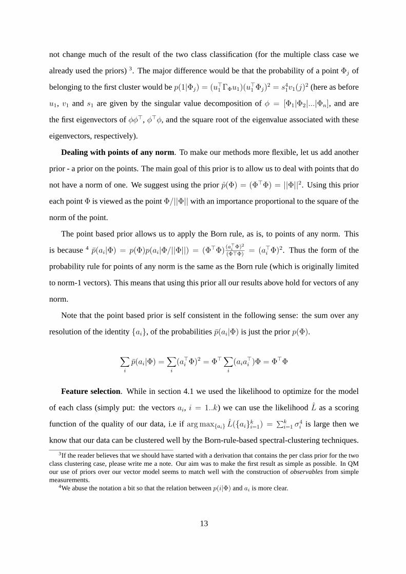
Dealing with points of any norm. To make our methods more flexible, let us add another

prior - a prior on the points. The main goal of this prior is to allow us to deal with points that do

not have a norm of one. We suggest using the priorp(Φ) = (Φ>Φ) = ||Φ||2. Using this prior

each pointΦ is viewed as the pointΦ/||Φ|| with an importance proportional to the square of the

norm of the point.

The point based prior allows us to apply the Born rule, as is, to points of any norm. This

is because4 p(ai|Φ) = p(Φ)p(ai|Φ/||Φ||) = (Φ>Φ)(a>i Φ)2

(Φ>Φ)= (a>i Φ)2. Thus the form of the

probability rule for points of any norm is the same as the Born rule (which is originally limited

to norm-1 vectors). This means that using this prior all our results above hold for vectors of any

norm.

Note that the point based prior is self consistent in the following sense: the sum over any

resolution of the identity{ai}, of the probabilitiesp(ai|Φ) is just the priorp(Φ).

∑

i

p(ai|Φ) =∑

i

(a>i Φ)2 = Φ> ∑

i

(aia>i )Φ = Φ>Φ

Feature selection. While in section 4.1 we used the likelihood to optimize for the model

of each class (simply put: the vectorsai, i = 1..k) we can use the likelihoodL as a scoring

function of the quality of our data, i.e ifarg max{ai} L({ai}ki=1) =

∑ki=1 σ4

i is large then we

know that our data can be clustered well by the Born-rule-based spectral-clustering techniques.

3If the reader believes that we should have started with a derivation that contains the per class prior for the twoclass clustering case, please write me a note. Our aim was to make the first result as simple as possible. In QMour use of priors over our vector model seems to match well with the construction ofobservablesfrom simplemeasurements.

4We abuse the notation a bit so that the relation betweenp(i|Φ) andai is more clear.

13

This allows us to “improve” our data5.

In the feature selection case we would like to select a subset of the variables such that the

resulting data would have a large score, i.e if we havel variables, we would like find binary

vectorα of l variables such that the sum of the fourth power of the singular values ofdiag(α)φ

is maximized. The diagonal matrixdiag(α) would determine which variables (rows ofφ) were

selected.

Optimizing that score over all possible assignments ofα is a problem of exponential com-

plexity. TheQ − α algorithm circumvents this problem by assigning positive weights√

α to

each one of the variables, where0 ≤ αi ≤ 1. The optimization problem then becomes:

maxα

k∑

i=1

σ4i = maxα

k∑

i=1

(vα>i φ>D(α)φvα

i )2 = maxα,Q

k∑

i=1

(q>i φ>D(α)φqi)2 =

= maxα,QTr(Q>(φ>D(α)φ)(φ>D(α)φ)Q) ,

whereVα = [vα1 |..|vα

k ] is the matrix of the eigenvectors ofφ>D(α)φ, and whereQ =

[q1|..|qk] is constrained to be ann (the number of the vectorsΦj) timesk (number of clusters)

matrix with orthonormal columns. The above score is dependent on the scale ofα, and so the

norm ofα is restricted to be one. Note that no restrictions are put onα to make it a vector of

positive entries. Still, the vectorα which maximizes the score is very likely to have all entries

which are of the same sign. This property, along with arguments predicting sparsity of the

entries ofα, can be found in [31].

The optimization of the scoremaxα,QTr(Q>(φ>D(α)φ)(φ>D(α)φ)Q) is carried using an

iterative algorithm which interweaves the computation ofα and improvements of the matrixQ.

Details can be found in [31].

5It would be interesting to compare the simple score we derived here of the quality of the data to the one thatcan be derived using Gaussian Processes [16]. If we consider a Gaussian Process with a kernelC of sizen × n,then the most likely orthogonal set ofk data-points would be the firstk eigenvectors ofC. This can be usedto give a partial explanation for the success of spectral clustering. The likelihood of thesek data-points (givenas columns of the matrix t) would beL = −1/2 log det C − 1/2Tr(t>C−1t) − n/2 log 2π = log Πn

i=1σ2i −

1/2∑k

i=1 1/σ2i − n/2 log 2π. Likelihoods of this sort are often optimized in the Gaussian Process literature, but

only for a few parameters. This is done in the supervised case, where t is the actual data, and the missing parameteris, for example, the width of the Gaussian. It is by far less tractable to optimize than our simple score.

14

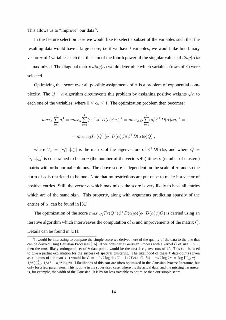
In casek is unknown, we may choose to assume it equalsn. This is because in our

score smaller singular values contribute much less than the larger ones. In the case where

k = n there is no need to optimize for the eigenvectorsQ and the score simply becomes

Tr(φ>D(α)φφ>D(α)φ) =∑

i,j αiαj(Φ>i Φj)

2. This bilinear problem is optimized whenα is

the first eigenvector of the matrix whose (i,j)-th element is(Φ>i Φj)

2.

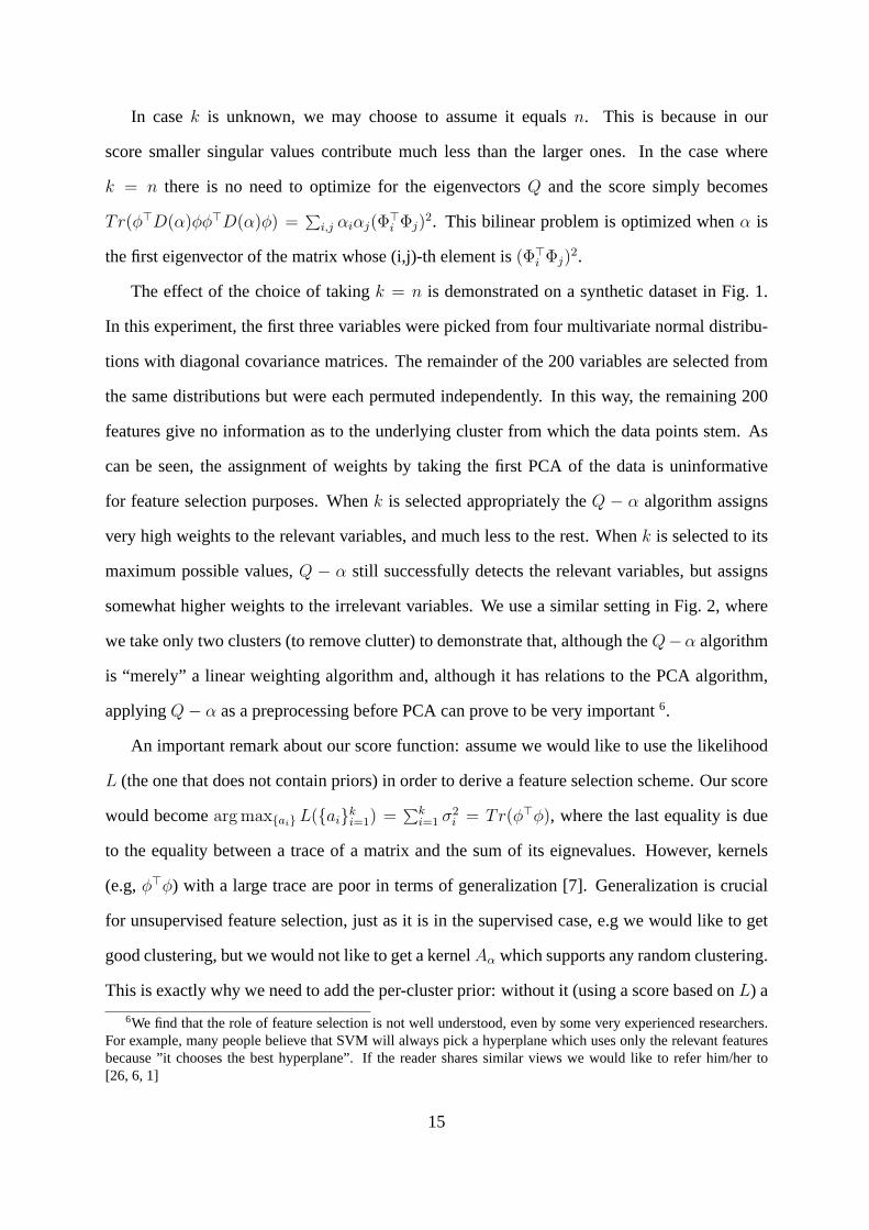
The effect of the choice of takingk = n is demonstrated on a synthetic dataset in Fig. 1.

In this experiment, the first three variables were picked from four multivariate normal distribu-

tions with diagonal covariance matrices. The remainder of the 200 variables are selected from

the same distributions but were each permuted independently. In this way, the remaining 200

features give no information as to the underlying cluster from which the data points stem. As

can be seen, the assignment of weights by taking the first PCA of the data is uninformative

for feature selection purposes. Whenk is selected appropriately theQ − α algorithm assigns

very high weights to the relevant variables, and much less to the rest. Whenk is selected to its

maximum possible values,Q − α still successfully detects the relevant variables, but assigns

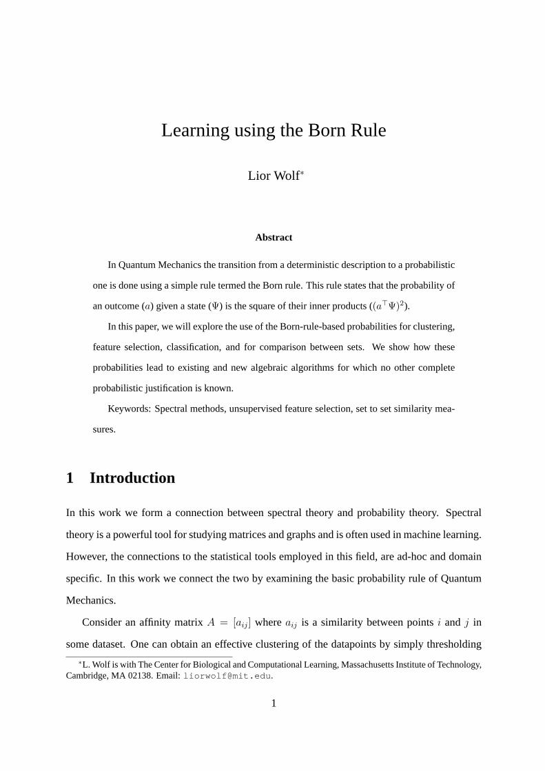
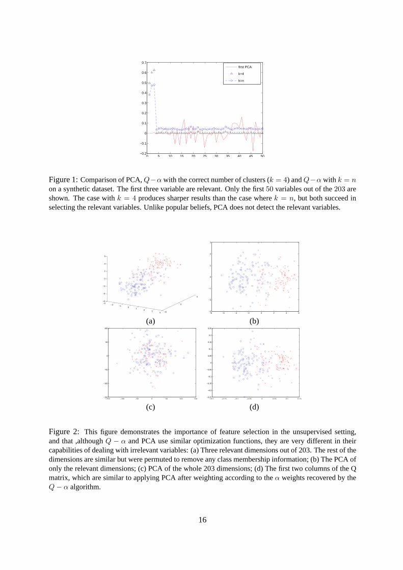
somewhat higher weights to the irrelevant variables. We use a similar setting in Fig. 2, where

we take only two clusters (to remove clutter) to demonstrate that, although theQ−α algorithm

is “merely” a linear weighting algorithm and, although it has relations to the PCA algorithm,

applyingQ− α as a preprocessing before PCA can prove to be very important6.

An important remark about our score function: assume we would like to use the likelihood

L (the one that does not contain priors) in order to derive a feature selection scheme. Our score

would becomearg max{ai} L({ai}ki=1) =

∑ki=1 σ2

i = Tr(φ>φ), where the last equality is due

to the equality between a trace of a matrix and the sum of its eignevalues. However, kernels

(e.g,φ>φ) with a large trace are poor in terms of generalization [7]. Generalization is crucial

for unsupervised feature selection, just as it is in the supervised case, e.g we would like to get

good clustering, but we would not like to get a kernelAα which supports any random clustering.

This is exactly why we need to add the per-cluster prior: without it (using a score based onL) a

6We find that the role of feature selection is not well understood, even by some very experienced researchers.For example, many people believe that SVM will always pick a hyperplane which uses only the relevant featuresbecause ”it chooses the best hyperplane”. If the reader shares similar views we would like to refer him/her to[26, 6, 1]

15

0 5 10 15 20 25 30 35 40 45 50−0.2

−0.1

0

0.1

0.2

0.3

0.4

0.5

0.6

0.7first PCA

k=4

k=n

Figure 1:Comparison of PCA,Q−α with the correct number of clusters (k = 4) andQ−α with k = non a synthetic dataset. The first three variable are relevant. Only the first50 variables out of the203 areshown. The case withk = 4 produces sharper results than the case wherek = n, but both succeed inselecting the relevant variables. Unlike popular beliefs, PCA does not detect the relevant variables.

−3−2

−10

12

34 −5

0

5

−6

−4

−2

0

2

4

6

−8 −6 −4 −2 0 2 4 6−3

−2

−1

0

1

2

3

(a) (b)

−150 −100 −50 0 50 100 150−150

−100

−50

0

50

100

−0.2 −0.15 −0.1 −0.05 0 0.05 0.1 0.15−0.25

−0.2

−0.15

−0.1

−0.05

0

0.05

0.1

0.15

0.2

0.25

(c) (d)

Figure 2: This figure demonstrates the importance of feature selection in the unsupervised setting,and that ,althoughQ − α and PCA use similar optimization functions, they are very different in theircapabilities of dealing with irrelevant variables: (a) Three relevant dimensions out of 203. The rest of thedimensions are similar but were permuted to remove any class membership information; (b) The PCA ofonly the relevant dimensions; (c) PCA of the whole 203 dimensions; (d) The first two columns of the Qmatrix, which are similar to applying PCA after weighting according to theα weights recovered by theQ− α algorithm.

16

clustering where every point is a cluster by itself would be considered a good clustering. Using

the per-cluster prior, each such one-point-cluster would have a very low prior, and the score

based on the likelihoodL will be much lower.

Note that in theQ − α algorithm, the trace of the kernel is controlled by the constraint on

the norm ofα: Let fi, i = 1..l be thel rowsof the matrixφ = [Φ1|...|Φn]. The kernel matrix

can be written as a sum of rank one matricesφ>diag(α)φ =∑l

k=1 αkfkf>k , each with a trace

Tr(fkf>k ) = f>k fk, and so the trace of the kernel matrixTr(φ>diag(α)φ) =

∑lk=1 αlf

>k fk.

Before application of theQ−α algorithm we usually normalize eachfk to have a norm of one,

so that the results will be independent of the scale of each feature. Hence the trace of the kernel

matrix is just∑

l αl. Under the constraint thatα has a norm of one, this trace is larger when

theα vector is more uniform. However, the maximization of the score function based on the

squares of the eigenvalues of the kernel matrix encourages a sparse solution [31].

4.3 Set to Set similarities

Another machine learning tool that we consider is the construction of a similarity function

between two sets of norm-1 vectors. Given a matrixφ whose columns are the vectors in our

set{Φi}ni=1, we can view it as a set of pure states, or alternatively as the mixed stateΓΦ =

(1/n)φφ> = (1/n)∑n

i=1 ΦiΦ>i .

Given a new set{Ψj}mj=1, we would like to find a similarity between the two sets. Letψ be

a matrix whose columns are the vectors of the new set. We can use, for example, either one of

these similarity measures:

(a) 1m

∑mj=1 Ψ>

j ΓΦΨj = 1nm

∑ni=1

∑mj=1(Φ

>i Ψj)2 = 1

nm ||φT ψ||2F

(b) 1m

∑m

j=1Ψ>j ΓΦΓΦΨj

Tr(ΓΦΓΦ) = 1mTr(φφ>)

∑ni,j=1

∑mk=1(Φ

>i Φj)(Φ>i Ψk)(Φ>j Ψk) = 1

nm||φφT ψ||2F||φφT ||2F

These similarities are based on applying the Born rule in its simplest form. However, they

are unnatural in the sense that if we model set elements as states, then it seems that we apply

the Born rule not between a state and a measurement but between two states. The underlying

reason is quite simple: the measurement that maximizes the distinguishably of a state (Φ) from

17

other states has the same vector representation asΦ [33].

Method (a) therefore measures the expectation of observing on the second set of measur-

ments that best identify the pure states which appear in the first set. However, this does not give

the best global measure of identifying the setφ in the following sense: It does not maximize the

expectation1n

∑ni=1 Φ>

i ρΦi subject toρ being a density matrix.

This expectation is maximized by lettingρ = aa> wherea is the first eigenvector ofΓΦ

7. However, to measure the similarity of two sets by just considering one observation does not

produce good results. The underlying problem is the problem of over-fitting, and is somewhat

similar to the need for regularization in the Expected Risk Minimization framework.

Method (b) is a trade off between maximizing the expectancy above8 and having a more

“round” similarity measure. The measurements used in similarity (b) are the columns of the

matrixΓΦ, which are weighted combinations of the measurements used in (a).

Although both methods were derived in an asymmetric way, that is, treating one set as the

target set, and another as a set that needs to be distinguished from it, the similarity method

(a) is a positive definite similarity measuresbetween sets. Therefore it can be used together

with any kernel based learning algorithms. To see this property it is enough to note that

(1/nm)∑

ij(Φ>i Ψi)

2 = (1/nm)∑

ij(χ(Φi)>χ(Ψi)) = (1/nm)(

∑i χ(Φi))(

∑j χ(Ψj)), where

χ is a mapping from a vector to the vector of all its second order monomials. This positive

definite similarity function between sets is a different one than the one described in [30], where

the determinant of the matrixφ>ψ and similar functions where used.

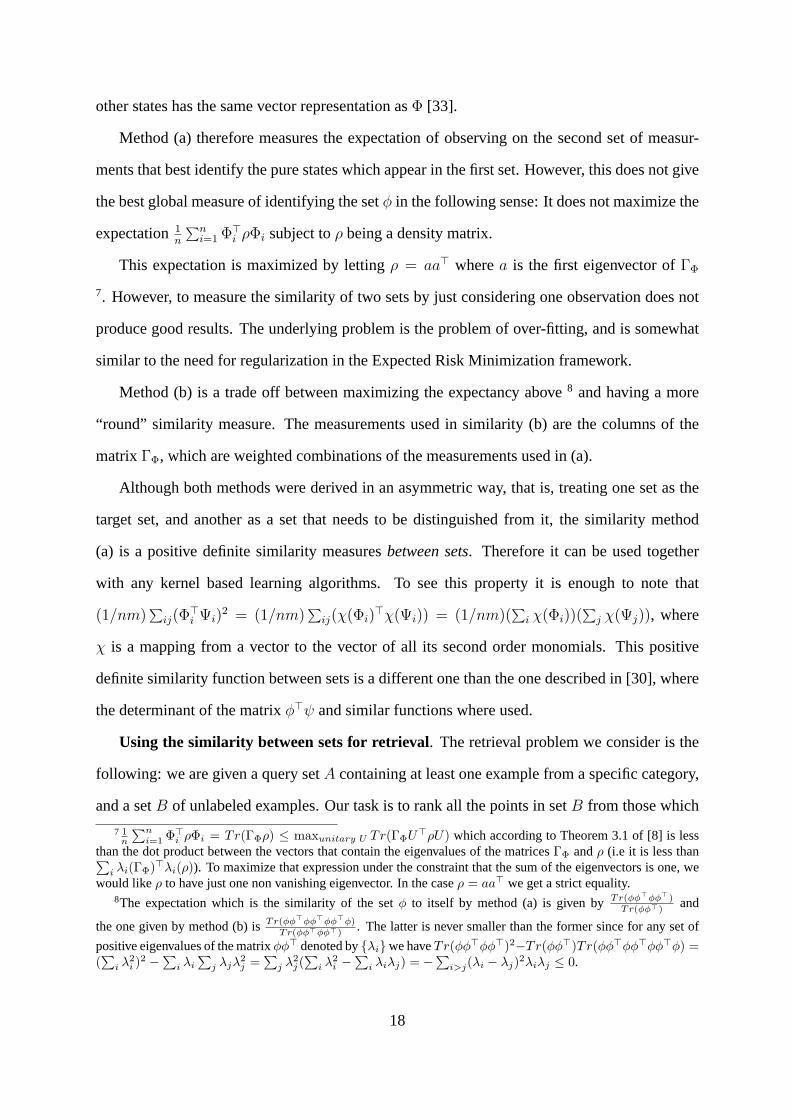
Using the similarity between sets for retrieval. The retrieval problem we consider is the

following: we are given a query setA containing at least one example from a specific category,

and a setB of unlabeled examples. Our task is to rank all the points in setB from those which

7 1n

∑ni=1 Φ>i ρΦi = Tr(ΓΦρ) ≤ maxunitary U Tr(ΓΦU>ρU) which according to Theorem 3.1 of [8] is less

than the dot product between the vectors that contain the eigenvalues of the matricesΓΦ andρ (i.e it is less than∑i λi(ΓΦ)>λi(ρ)). To maximize that expression under the constraint that the sum of the eigenvectors is one, we

would likeρ to have just one non vanishing eigenvector. In the caseρ = aa> we get a strict equality.8The expectation which is the similarity of the setφ to itself by method (a) is given byTr(φφ>φφ>)

Tr(φφ>)and

the one given by method (b) isTr(φφ>φφ>φφ>φ)Tr(φφ>φφ>)

. The latter is never smaller than the former since for any set of

positive eigenvalues of the matrixφφ> denoted by{λi}we haveTr(φφ>φφ>)2−Tr(φφ>)Tr(φφ>φφ>φφ>φ) =(∑

i λ2i )

2 −∑i λi

∑j λjλ

2j =

∑j λ2

j (∑

i λ2i −

∑i λiλj) = −∑

i>j(λi − λj)2λiλj ≤ 0.

18

are more likely to be of the same category of the examples in setA to those that are less likely.

Below we offer two methods, RMa and RMb.

The first method (RMa) treats each point as a set of one point and ranks each point inB by

its similarity using the set similarity method (a) to the set of labeled pointsA. The points in set

B are then ranked from the most similar point to the least similar point. This method is very

simple, but it does not incorporate information on the structure of setB until the last stage of

sorting the per-point similarity scores.

The second method (RMb) weights each pointi in setB by a weight√

αi, and tries to

maximize the similarity between the resulting set and setA 9. Thus we search for a vector

α which maximizes||φdiag(α)φ>ψ||2F||φdiag(α)φ>||2F

, where the matrixφ holds the elements of setB and the

matrix ψ holds the elements of setA. Both the numerator and the denominator are clearly

bilinear inα and so this can be written asα>Gαα>Hα

, the maximization of which is just a generalized

eigenvector problem, and is given up to scale. Following the algebra one can verify thatG[ij] =

∑k(Φ

>i Φk)(Φ

>i Ψj)(Φ

>k Ψj), andH[ij] = (Φ>

i Φj)2.

The ranking is by sorting of the values ofα. We set the sign of the value ofα which has the

largest magnitude to be positive, and sort all of theα values to get a ranking of all the examples

in setB. Note that, although it is not guaranteed that the entries of the vectorα would be all of

the same sign, in almost all of the experiments we ran this was the case. If some of the values

happened to differ in sign from the value which had the largest magnitude, in our experience

they were of a very small magnitude.

Note that RMb examines not only the similarity of single elements in setB to setA but tries

to find the subset ofB which is the most similar toA. Also, note that the set-to-set similarity

(b) is normalized such that sets which are very similar to themselves (highly clustered) are

penalized in the denominator of this similarity, giving balance to this similarity score.

9A similar method using set similarity (a) would result in method RMa. This is because the solution forarg maxα ||ψ>φdiag(

√α)||2F , s.t||α|| = 1 is proportional to the vector with elements||ψ>Φi||2F .

19

4.4 Classification

There are several ways in which one can derive classification algorithms based on Born rule

probabilities. Here we will derive an existing classifier which is very similar to the use of

density kernel estimators [14] for classification. This is an effective classification method, and

we are going to base it on the set to set similarity (a) given above. Our derivation method is

designed for norm-1 vectors only. In practice we normalize the vectors with accordance to the

kernel used (e.g normalize each vector by its norm for the linear kernel), or simply use an RBF

kernel.

Given a set ofn positive examples, as columns of a matrixφ, we can for any new example

Ψ compute the similarity according to method (a) aboveO+(Ψ) = 1n||φT Ψ||2. This measure of

similarity is a normalized expectation, and we can use a simple ratio test to classify the pointΨ.

i.e we classifyΨ to have a positive label ifO+(Ψ)1−O+(Ψ)

> 1.

Given a set of negative examples we can build a second measureO− and combine those

using the naıve Bayes approach. The classification engine we use in the experiments below

simply checks if: O+(Ψ)1−O+(Ψ)

1−O−(Ψ)O−(Ψ)

> 1. This is a very simple plug-in decision rule, which

requires virtually no training. As a plug-in classifier it generalizes well [11].

5 Experiments

The clustering algorithm we suggest amounts to a variant of spectral clustering which was ex-

tensively studied [27, 18]. Therefore we will not present extensive new clustering experiments.

However, there is a point we would like to make about classification of out-of-sample points.

Since we use a model-based approach our clustering can be applied to any new point without

re-clustering. This is in contrast to the original NJW algorithm and to the original Laplacian

Eigenmaps [4]. To overcome this problem, a term of regularization was recently added to the

Laplacian Eignemaps algorithm [5].

In our framework out of sample extensions come naturally since for any new pointΨ we

can compute out model based probabilities. These probabilities can be expressed as function

20

−1 −0.5 0 0.5 1 1.5 2 2.5

−0.6

−0.4

−0.2

0

0.2

0.4

0.6

0.8

1

1.2

−1 −0.5 0 0.5 1 1.5 2 2.5

−0.6

−0.4

−0.2

0

0.2

0.4

0.6

0.8

1

1.2

(a) (b)

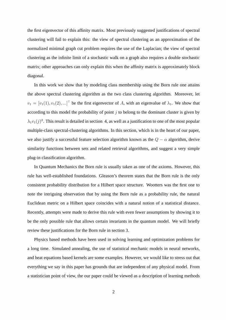
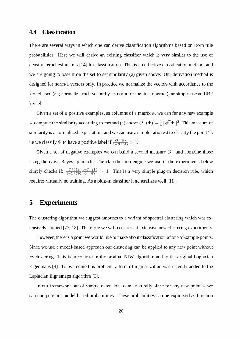
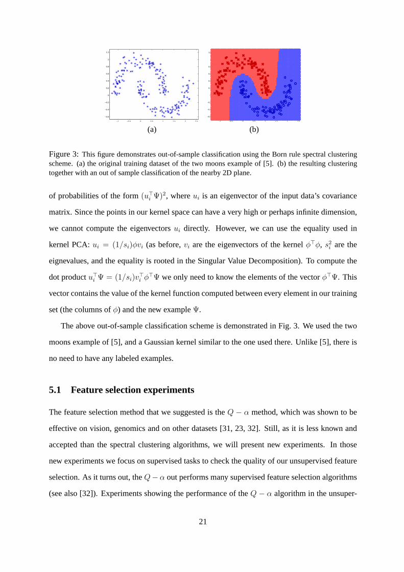
Figure 3:This figure demonstrates out-of-sample classification using the Born rule spectral clusteringscheme. (a) the original training dataset of the two moons example of [5]. (b) the resulting clusteringtogether with an out of sample classification of the nearby 2D plane.

of probabilities of the form(u>i Ψ)2, whereui is an eigenvector of the input data’s covariance

matrix. Since the points in our kernel space can have a very high or perhaps infinite dimension,

we cannot compute the eigenvectorsui directly. However, we can use the equality used in

kernel PCA:ui = (1/si)φvi (as before,vi are the eigenvectors of the kernelφ>φ, s2i are the

eignevalues, and the equality is rooted in the Singular Value Decomposition). To compute the

dot productu>i Ψ = (1/si)v>i φ>Ψ we only need to know the elements of the vectorφ>Ψ. This

vector contains the value of the kernel function computed between every element in our training

set (the columns ofφ) and the new exampleΨ.

The above out-of-sample classification scheme is demonstrated in Fig. 3. We used the two

moons example of [5], and a Gaussian kernel similar to the one used there. Unlike [5], there is

no need to have any labeled examples.

5.1 Feature selection experiments

The feature selection method that we suggested is theQ − α method, which was shown to be

effective on vision, genomics and on other datasets [31, 23, 32]. Still, as it is less known and

accepted than the spectral clustering algorithms, we will present new experiments. In those

new experiments we focus on supervised tasks to check the quality of our unsupervised feature

selection. As it turns out, theQ−α out performs many supervised feature selection algorithms

(see also [32]). Experiments showing the performance of theQ − α algorithm in the unsuper-

21

vised case are presented in the conference papers [31, 23]. Since we did not want to optimize

over the free parameter used for the feature selectionk (generally referred to as the number of

classes), we present results in the case wherek = n (n being the number of examples at hand).

In this case theQ − α algorithm is non-iterative, so there is also a considerable saving of run

time.

Face Recognition. We first appliedQ − α for the task face recognition. We used two

publicly available datasets: the YALE dataset [34] and the AR dataset [17]. The YALE dataset

contains 15 different persons, each one photographed 11 times under different illumination,

with different expression and with or without glasses. For the AR dataset we used only the 25

males, each having 52 images. For both datasets we created 20 instances of similar experiments,

where three images per person were picked randomly to be the training set for that person. The

rest served as the test set.

We compared several algorithms: the eigenface method [25] which uses PCA to reduce the

dimension of the face images; the fisherface method [3] which applies multi-class Fisher dis-

criminant analysis (FDA) to face images after they have been reduced in dimension using PCA;

both methods after applying conventional feature selection algorithms ; an application of eigen-

faces after variable weighting using theQ − α algorithm; and application of fisherfaces after

variable weighting using theQ− α algorithm. All methods where tested for gray level images

and for wavelet. Results in the table are the maximal score out of these two options. These

results are only higher for gray values when using the variants without any feature selection.

Q − α and the other feature selection methods did not seem to work well when dealing with

gray level values directly10. In order to remove any doubt, we would like to emphasize again

that the results were not biased by using different kinds of features. Each method was tested on

10In the heart of these phenomena lies a basic discrepancy between feature selection and dimensionality reduc-tion algorithms. While feature selection algorithms (Fisher score,Q− α , and in a sense Ada-boost) do well withuncorrelated data, they perform much worse when many of the features are correlated. Dimensionality reductionalgorithms (PCA, FDA, and in a sense SVM) thrive on correlation, but fail when dealing with a large numberof uncorrelated features. Gray values are highly correlated, therefore PCA, FDA and SVM work well on them.Wavelets are not correlated, and therefore are more suitable for boosting, feature selection, and naıve baysian ap-proaches. As shown in the experiments, theQ − α algorithm enables PCA, SVM and FDA to work with waveletfeatures (In the past wavelets and SVM were combined for pedestrian detection [19]. For that end a correlatedover-complete wavelet basis was used).

22

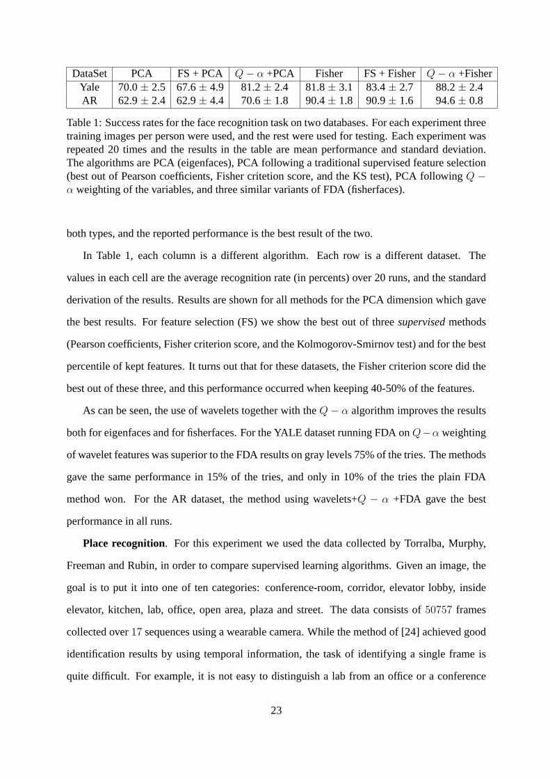
DataSet PCA FS + PCA Q− α +PCA Fisher FS + Fisher Q− α +FisherYale 70.0± 2.5 67.6± 4.9 81.2± 2.4 81.8± 3.1 83.4± 2.7 88.2± 2.4AR 62.9± 2.4 62.9± 4.4 70.6± 1.8 90.4± 1.8 90.9± 1.6 94.6± 0.8

Table 1: Success rates for the face recognition task on two databases. For each experiment threetraining images per person were used, and the rest were used for testing. Each experiment wasrepeated 20 times and the results in the table are mean performance and standard deviation.The algorithms are PCA (eigenfaces), PCA following a traditional supervised feature selection(best out of Pearson coefficients, Fisher critetion score, and the KS test), PCA followingQ −α weighting of the variables, and three similar variants of FDA (fisherfaces).

both types, and the reported performance is the best result of the two.

In Table 1, each column is a different algorithm. Each row is a different dataset. The

values in each cell are the average recognition rate (in percents) over 20 runs, and the standard

derivation of the results. Results are shown for all methods for the PCA dimension which gave

the best results. For feature selection (FS) we show the best out of threesupervisedmethods

(Pearson coefficients, Fisher criterion score, and the Kolmogorov-Smirnov test) and for the best

percentile of kept features. It turns out that for these datasets, the Fisher criterion score did the

best out of these three, and this performance occurred when keeping 40-50% of the features.

As can be seen, the use of wavelets together with theQ− α algorithm improves the results

both for eigenfaces and for fisherfaces. For the YALE dataset running FDA onQ−α weighting

of wavelet features was superior to the FDA results on gray levels 75% of the tries. The methods

gave the same performance in 15% of the tries, and only in 10% of the tries the plain FDA

method won. For the AR dataset, the method using wavelets+Q − α +FDA gave the best

performance in all runs.

Place recognition. For this experiment we used the data collected by Torralba, Murphy,

Freeman and Rubin, in order to compare supervised learning algorithms. Given an image, the

goal is to put it into one of ten categories: conference-room, corridor, elevator lobby, inside

elevator, kitchen, lab, office, open area, plaza and street. The data consists of50757 frames

collected over17 sequences using a wearable camera. While the method of [24] achieved good

identification results by using temporal information, the task of identifying a single frame is

quite difficult. For example, it is not easy to distinguish a lab from an office or a conference

23

room.

Each frame in the place recognition dataset was represented by a vector of384 dimensions,

consisting of the output of steerable filters applied to the input120 × 160 image at several

scales. This representation, together with the frame annotation, was made publicly available by

the authors of [24].

We conducted repeated one-vs-all experiments. In each experiment 100 random examples

of one place catagory served as the set of positive training examples, and 100 random examples

from the rest of the frames served as negative examples. The results were then tested on a

much larger set of testing examples, which contained the same number of positive and negative

examples. Each such one-vs-all experiment was repeated three times.

In [24] the authors used the gentle boost algorithm on top of PCA. In our experiments, SVM

always outperfoms the boosting algorithm (we used the same implementation, provided to us

by Torralba). This is probably due to a relatively small number of training examples used in

our experiments. Also, in all our experiments, PCA did not help at all (not even for boosting),

hence we used the original384 dimensional data.

The results we got are26.67% percent error for an 80 dimensional PCA followed by a

linear SVM,25.10% for a linear SVM, and23.17% error forQ − α weighting of the features

followed by an SVM. We could improve the results a bit by applying a novel supervised version

of Q− α (not reported here) and get22.83% error.

5.2 Retrieval experiments

In order to check our retrieval experiments we compared three methods: ranking by distance to

the closest element in the query setA (NN), which is probably the most commonly used method;

ranking using RMa (the method based on set-to-set similarity a); and RMb (the method based on

set-to-set similarity b). To avoid any bias in favor of our method we only used the linear kernel

(NN could not be improved by a Guassian kernel, and we wanted to avoid the appearance of

tilting the results using multiple tests with several parameters ).

In the first set of experiments, we used datasets from the UCI machine learning repository.

24

Method NN RMa RMbSplitRatio 5% 10% 30% 5% 10% 30% 5% 10% 30%

Dermatology .51 .52 .52 .87 .87 .88 .83 .80 .78Ecoli .97 .97 .98 .92 .92 .95 .87 .91 .95Glass .44 .38 .36 .43 .36 .35 .62 .60 .62

Letter Recognition .68 .68 .68 .73 .74 .74 .90 .94 .96Segmentation .96 .96 .96 .90 .90 .95 .84 .84 .85

Wine .94 .93 .95 .80 .85 .88 .05 .04 .04Yeast .58 .58 .60 .57 .57 .60 .53 .54 .63

Table 2: Retrieval experiments on several UCI datasets

In each experiment only40% of each dataset was used (this is important to avoid bias because

RMb uses all the examples to determine the ranking). We split each partial (40%) dataset into

two setA andB for various sizes of setA. A split ratio of 20% means that20 percent of the

largest class were used as setA and the rest of all the examples as setB. Each such experiment

was repeated 20 times, and the average results are shown below. As a measure of success we

used the area under the resulting ROC curve generated by correct and incorrect retrievals from

setB.

The results are summarized in table 2. They show that for many datasets the methods RMa

and RMb preform significantly better than NN. However, this is not the case for all datasets.

Sometimes NN does better.

Note that in general, we should not expect a monotonic performance as setA grows, since

the ratio of positive examples in setB becomes worse. Also, note that sometimes method RMb

can “lock” onto the wrong class. This happens if the negative examples contain a very tight

cluster, while the positive ones are very loosely distributed.

Another set of retrieval experiments was conducted by Stan Bileschi. In out dataset we had

80 image patches taken from car images. These patches (“parts”) were selected automatically

using an interest operator (some are not specific to any car part like wheel or mirror, and are just

patches around the point given by the interest operator.). For each part we got 10-50 possible

matches in our image dataset, using normalized cross correlation with a predefined threshold.

Our goal was to use these possible matches to train a part classifier. We were hoping to get 20

25

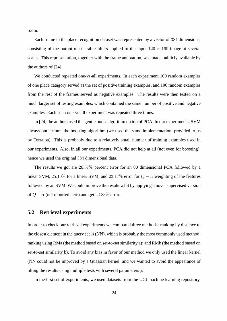
Method NN RMa RMbGray values 2.21 2.07 2.46

Wavelets 2.16 2.69 1.44

Table 3: Retrieval results for the car parts dataset. Entries show the average over all parts of theratio between the number of correct retrievals in the first 20 answers and the expected numberof retrievals .

positive training images for each part, which is enough to train a very reliable classifier.

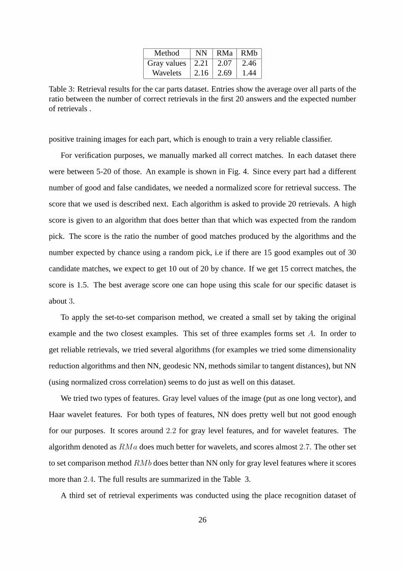
For verification purposes, we manually marked all correct matches. In each dataset there

were between 5-20 of those. An example is shown in Fig. 4. Since every part had a different

number of good and false candidates, we needed a normalized score for retrieval success. The

score that we used is described next. Each algorithm is asked to provide 20 retrievals. A high

score is given to an algorithm that does better than that which was expected from the random

pick. The score is the ratio the number of good matches produced by the algorithms and the

number expected by chance using a random pick, i.e if there are 15 good examples out of 30

candidate matches, we expect to get 10 out of 20 by chance. If we get 15 correct matches, the

score is 1.5. The best average score one can hope using this scale for our specific dataset is

about3.

To apply the set-to-set comparison method, we created a small set by taking the original

example and the two closest examples. This set of three examples forms setA. In order to

get reliable retrievals, we tried several algorithms (for examples we tried some dimensionality

reduction algorithms and then NN, geodesic NN, methods similar to tangent distances), but NN

(using normalized cross correlation) seems to do just as well on this dataset.

We tried two types of features. Gray level values of the image (put as one long vector), and

Haar wavelet features. For both types of features, NN does pretty well but not good enough

for our purposes. It scores around2.2 for gray level features, and for wavelet features. The

algorithm denoted asRMa does much better for wavelets, and scores almost2.7. The other set

to set comparison methodRMb does better than NN only for gray level features where it scores

more than2.4. The full results are summarized in the Table 3.

A third set of retrieval experiments was conducted using the place recognition dataset of

26

Figure 4: An example of a part in our dataset. A green box marks a good detection, a red box marksfalse detections. The task was to automatically find all good detections given the one example on theupper left corner

27

0 2 4 6 8 10 12 14 16 180.6

0.65

0.7

0.75

0.8

0.85

RMaRMbmean distanceNN

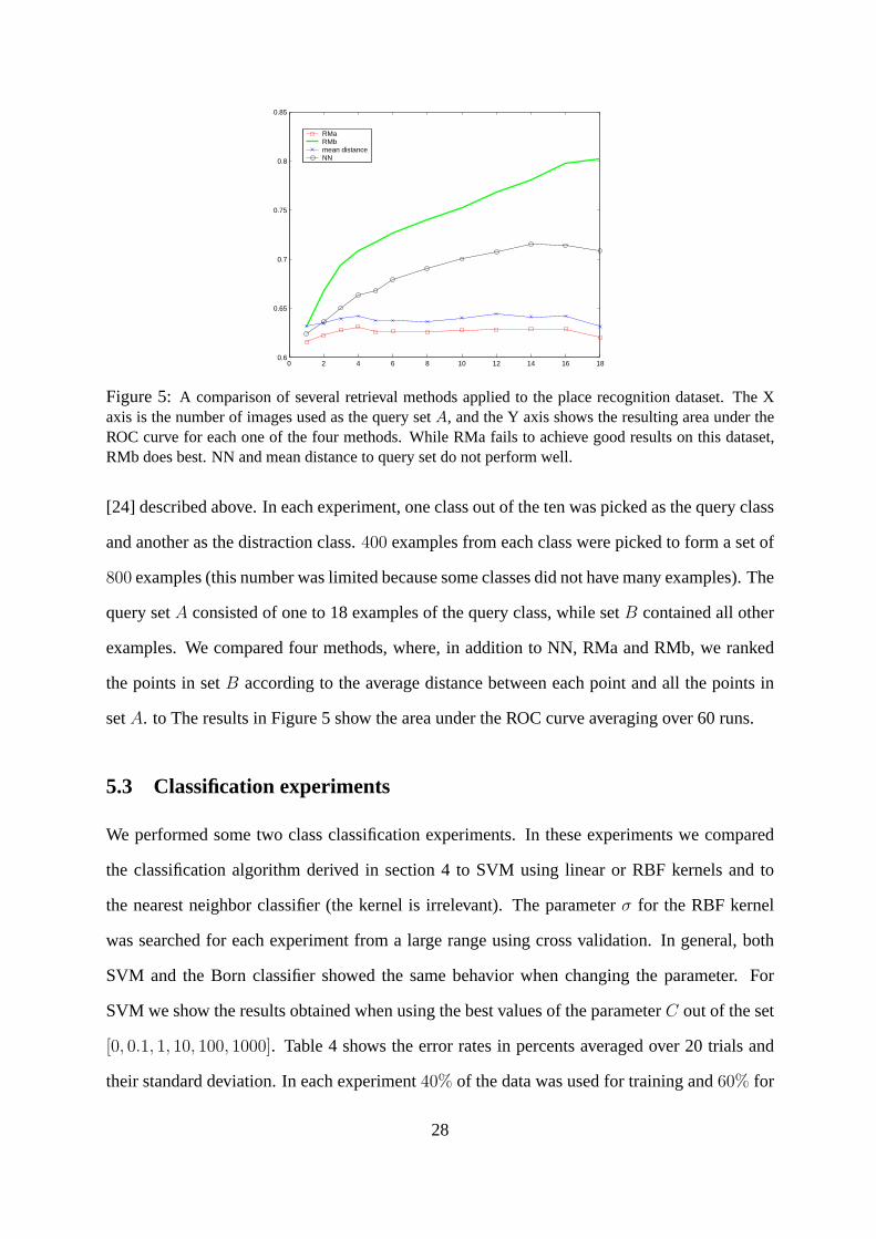
Figure 5: A comparison of several retrieval methods applied to the place recognition dataset. The Xaxis is the number of images used as the query setA, and the Y axis shows the resulting area under theROC curve for each one of the four methods. While RMa fails to achieve good results on this dataset,RMb does best. NN and mean distance to query set do not perform well.

[24] described above. In each experiment, one class out of the ten was picked as the query class

and another as the distraction class.400 examples from each class were picked to form a set of

800 examples (this number was limited because some classes did not have many examples). The

query setA consisted of one to 18 examples of the query class, while setB contained all other

examples. We compared four methods, where, in addition to NN, RMa and RMb, we ranked

the points in setB according to the average distance between each point and all the points in

setA. to The results in Figure 5 show the area under the ROC curve averaging over 60 runs.

5.3 Classification experiments

We performed some two class classification experiments. In these experiments we compared

the classification algorithm derived in section 4 to SVM using linear or RBF kernels and to

the nearest neighbor classifier (the kernel is irrelevant). The parameterσ for the RBF kernel

was searched for each experiment from a large range using cross validation. In general, both

SVM and the Born classifier showed the same behavior when changing the parameter. For

SVM we show the results obtained when using the best values of the parameterC out of the set

[0, 0.1, 1, 10, 100, 1000]. Table 4 shows the error rates in percents averaged over 20 trials and

their standard deviation. In each experiment40% of the data was used for training and60% for

28

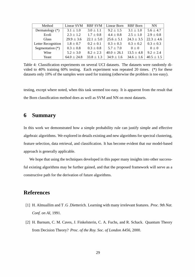
Method Linear SVM RBF SVM Linear Born RBF Born NNDermatology (*) 3.1± 1.0 3.0± 1.1 9.2± 1.5 3.1± 1.0 5.6± 4.7

Ecoli 2.3± 1.2 1.7± 0.8 4.4± 0.8 2.5± 1.0 2.9± 0.8Glass 29.9± 3.6 22.1± 5.0 25.6± 5.1 24.3± 3.5 22.3± 4.6

Letter Recognition 1.8± 0.7 0.2± 0.1 0.3± 0.3 0.3± 0.2 0.3± 0.3Segmentation (*) 0.3± 0.8 0.3± 0.8 5.7± 7.0 0± 0 0± 0

Wine 5.2± 3.0 8.2± 2.3 40.0± 26.1 13.5± 4.8 9.2± 2.4Yeast 64.0± 24.8 33.8± 1.3 34.9± 1.6 34.6± 1.6 40.5± 1.5

Table 4: Classification experiments on several UCI datasets. The datasets were randomly di-vided to 40% training 60% testing. Each experiment was repeated 20 times. (*) for thesedatasets only 10% of the samples were used for training (otherwise the problem is too easy).

testing, except where noted, when this task seemed too easy. It is apparent from the result that

the Born classification method does as well as SVM and NN on most datasets.

6 Summary

In this work we demonstrated how a simple probability rule can justify simple and effective

algebraic algorithms. We explored in details existing and new algorithms for spectral clustering,

feature selection, data retrieval, and classification. It has become evident that our model-based

approach is generally applicable.

We hope that using the techniques developed in this paper many insights into other success-

ful existing algorithms may be further gained, and that the proposed framework will serve as a

constructive path for the derivation of future algorithms.

References

[1] H. Almuallim and T .G .Dietterich. Learning with many irrelevant features.Proc. 9th Nat.

Conf. on AI, 1991.

[2] H. Barnum, C. M. Caves, J. Finkelsterin, C. A. Fuchs, and R. Schack. Quantum Theory

from Decision Theory?Proc. of the Roy. Soc. of London A456, 2000.

29

[3] P.N. Belhumeur, J.P. Hespanha and D.J. Kreigman Eigenfaces vs. Fisherfaces: Recogni-

tion Using Class Specific Linear ProjectionPAMI 19(7), 1992.

[4] M. Belkin, and P. Niyogi Laplacian Eigenmaps for Dimensionality Reduction and Data

Representation. InNeural Computation14, 2002.

[5] M. Belkin, P. Niyogi, and V. Sindhwani Manifold Regularization: a Geometric Framework

for Learning from Examples The University of Chicago CS Technical Report TR-2004-06.

[6] A. Blum and P. Langley. Selection of relevant features and examples in machine learning.

AI, 97(1-2), 1997.

[7] O. Bousquet, and D.J.L. Herrmann On the Complexity of Learning the Kernel Matrix.

NIPS, 2003.

[8] I.D. Coope and P.F. Renaud. Trace Inequalities with Applications to Orthogonal Regres-

sion and Matrix Nearness Problems. Research Report UCDMS2000/17, 2000.

[9] D. Deutsch. Quantum Theory of Probability and Decisions.Proc. of the Roy. Soc. A455,

1999.

[10] L. Devroye. A Course in Density Estimation. Birkhauser, 1987.

[11] L. Devroye, L. Gyorfi, G. Lugosi. A Probababilistic Theory of Pattern Recog. Springer,

1996.

[12] A. Gleason. Measures on the closed subspaces of a hilbert space. InJournal of Mathe-

matics and Mechanics 6, 885-894. 1957.

[13] G.H. Golub and C.F. Van Loan.Matrix computations. , 1989.

[14] T. Hastie, R. Tibshirani, J. H. Friedman The Elements of Statistical Learning Springer,

2001.

[15] D. Horn and A. Gottlieb, Algorithms for Data Clustering in Pattern Recognition Problems

based on Quantum Mechanics. InPhysical Review Letters88(1), 2002.

30

[16] D. Mackay, Introductino to Gaussain Processes. (A review paper). Available at:

http://www.inference.phy.cam.ac.uk/mackay/GP/

[17] A.M. Martinez and R. Benavente. The AR face database. Tech. Rep. 24, CVC, 1998.

[18] A.Y. Ng, M.I. Jordan, Y. Weiss. On Spectral Clustering: Analysis and an algorithm.

NIPS,2001.

[19] M. Oren, C. Papageorgiou, P. Sinha, E. Osuna and T. Poggio. Pedestrian Detection Using

Wavelet Templates. InCVPR 1997.

[20] P. Perona and W. T. Freeman. A factorization approach to grouping. InECCV, 1998.

[21] S. Saunders. Operational Derivation of the Born Rule. in submission.

[22] B. Scholkopf and A.J. Smola.Learning with KernelsThe MIT press, 2002.

[23] A. Shashua and L. Wolf. Kernel Feature Selection with Side Data using a Spectral Ap-

proach. Proc. of the European Conference on Computer Vision (ECCV), May 2004

[24] A. Torralba, K. P. Murphy, W. T. Freeman, and M. A. Rubin. Context-based vision system

for place and object recognition, IEEE Intl. Conference on Computer Vision (ICCV),

2003.

[25] M. Turk and Pentland ”Face Recognition Using Eigenfaces”, InICPR, 1991.

[26] Weston, J., S. Mukherjee, O. Chapelle, M. Pontil, T. Poggio and V. Vapnik. Feature

Selection for SVMs.NIPS, 2001.

[27] D. Verma and M. Meila. A comparison of spectral clustering algorithms. UW CSE T.R.,

2003.

[28] D. Wallace, Everettian Rationality: defending Deutsch’s approach to probability in the

Everett interpretation. InStudies in the History and Philosophy of Modern Physics34,

2003.

31

[29] Y. Weiss. Segmentation using eigenvectors: a unifying view. InICCV, 1999.

[30] L. Wolf and A. Shashua. Learning over Sets using Kernel Principal Angles. InJMLR, 4,

2003.

[31] L. Wolf and A. Shashua. Direct feature selection with implicit inference.ICCV, 2003.

[32] L. Wolf, A. Shashua and S. Mukherjee. Selecting Relevant Genes with a Spectral Ap-

proach. AI MEMO AIM-2004-002

[33] W.K. Wootters. Statistical distance and Hilbert space. InPhysical Review D, 1991.

[34] Yale Univ. Face Database. Available at http://cvc.yale.edu/projects/yalefaces/yalefaces.html

[35] S. Zhong and J. Ghosh A Unified Framework for Model-based Clustering. JMLR 4, 2003

32