Embed Size (px)
Citation preview

Learning and Market Clearing: Theory and Experiments∗
Carlos Alos–Ferrer† and Georg Kirchsteiger‡
This version: February 2013
Abstract
This paper investigates theoretically and experimentally whether traders learn to use
market-clearing trading institutions or whether other (inefficient) market institutions can
survive in the long run. Using a framework with boundedly rational traders, we find that
market clearing institutions are always stable under a general class of learning dynamics.
However, we show that there exist other, non-market clearing institutions that are also
stable. Therefore, in the long run traders may fail to coordinate exclusively on market
clearing institutions. Using a replica-economies approach, we find the results to be robust to
large market size. The theoretical predictions were confirmed in a series of platform choice
experiments. Traders coordinated on platforms predicted to be stable, including market-
clearing as well as non-market clearing ones, while platforms predicted to be unstable were
avoided in the long run. (JEL C72, D4, D83)
Keywords: Market Institutions, Market Clearing, Coordination, Learning
∗We thank Ana B. Ania, Luis Corchon, Michihiro Kandori, Akihiko Matsui, Alex Possajennikov, and JorgenWeibull for helpful comments and suggestions.
†Department of Economics, University of Cologne. Albertus-Magnus Platz, D-50923 Cologne (Germany).Tel. (+49) 221 470 8303, Fax. (+49) 470 8321, email. [email protected]
‡ECARES, Universite Libre de Bruxelles. Avenue F. D. Roosevelt 50, CP114. 1050 Brussels (Belgium).Tel. (+32) 2 650 42 12, Fax. (+32) 2 650 44 75, email. [email protected]
1

Alos-Ferrer and Kirchsteiger Learning and Market Clearing
1 Introduction
The formation of a market requires a group of agents, some of them willing to buy and some of
them willing to sell. Preferences and cost functions are sufficient to develop a theory if market
clearing is taken as granted. Actual markets, though, are not merely characterized by demand
and supply. Market exchange requires an institutional framework in which action and message
sets are specified, and in which a process of matching and price formation can take place.
An enormous variety of market institutions can be observed in the field, even for the same
good. Both call markets and continuous double auction markets are used to exchange financial
assets. Real estate is sold both at auctions and by means of direct negotiations. In some
countries’ rental markets, established but informal institutions (e.g. group tenant visits) bias
the market in favor of the owners. In other countries, middlemen act as platforms which compete
actively for tenants. In addition there is always an alternative “word-of-mouth” market tenants
might resort to.
These details of the market institution are consequential. In addition to theoretical and
empirical evidence, there is a large body of experimental evidence in this direction.1 Trading
rules affect the efficiency of the market outcome, the convergence towards equilibrium, the
volatility of the prices, and the distribution of surplus over the market participants. Given that
“institutions matter” and given the competition between different market institutions, we might
ask which institutions are used in the long run. What are the properties of successful institutions?
Do the surviving market institutions support market clearing and efficient outcomes? Are there
circumstances under which inefficient trading rules can persist, or are forces and mechanisms
present that drive a market towards efficient organization?
Internet auction platforms like eBay, Yahoo, and Amazon provide a good example of compe-
tition between different market institutions. The trading rules of these auctions platforms differ
e.g. in their ending rules and in the type of the Buy-Now option sellers may use. Experimental
(Ariely, Ockenfels, and Roth, 2005) and theoretical analysis (Reynolds and Wooders, 2009) re-
veals that the level of realized prices as well as efficiency are influenced by these differences. A
similar conclusion can be drawn for the possibility of secret reserve prices (Bajari and Hortacsu,
2003) and for buy prices (Budish and Takeyama, 2001). In the context of multi-unit auctions,
Ausubel and Cramton (2002) show that uniform and pay-as-bid auctions lead to different real-
ized prices. Hence, competing institutions differ not only in their institutional setup, but the
different institutional setups lead to systematic differences in the realized prices.
The survival of a specific market institution depends on whether traders employ this insti-
tution or avoid it. The decision about the use of a particular market institution gives rise to a
game that combines aspects of a coordination and a minority game. On the one hand, poten-
1An overview of the classical experimental evidence on the importance of market institutions is provided byPlott (1982) (see also Holt, 1995).
2

Alos-Ferrer and Kirchsteiger Learning and Market Clearing
tial buyers and sellers have to coordinate on a particular institution in order to make mutual
beneficial trade possible. On the other hand, a trader is better off the fewer competing traders
opt for the same trading platform. Due to the coordination aspect such a game exhibits a mul-
tiplicity of Nash equilibria. All the traders might coordinate on an institution that does not
lead to market clearing outcomes. They might even coordinate on an institution that leads to
a Pareto-inefficient outcome. Hence, we ask under what circumstances traders will indeed learn
to coordinate on an efficient, market-clearing institution.
To provide an answer to this question, we conducted a theoretical and experimental study
of a market for a homogeneous good. Potential traders have to choose simultaneously at which
institution they want to trade. They choose between a market clearing institution and other
institutions that do not lead to market clearing, but realize other prices. Traders who have
chosen such an institution might obtain more favorable prices but necessarily face rationing. The
theoretical part of the analysis is based on a learning model where each trader has a tendency to
switch from one institution to a different one next period if another institution exhibits better
current-period results. Traders evaluate the results according to evaluation functions that satisfy
a number of weak behavioral assumptions, compatible with standard microeconomic models but
allowing also for boundedly rational behavior. The learning model is related to stochastic models
of learning in games (see Fudenberg and Levine, 1998, for an overview). In particular, traders
are not assumed to anticipate future prices, market-clearing or otherwise. They tend to switch
to strategies (institutions) which are better in the current period, without anticipating the
effects of their strategy change. Within this framework the market clearing institution is always
stochastically stable independently of the characteristics and the number of the other available
institutions. This strong prediction, however, does not imply that only market clearing will be
observed in the long run. On the contrary, we find that certain non-market clearing institutions
are also stochastically stable. Hence, the theoretical analysis suggests that in the long run
market-clearing institutions will be used, but in general not exclusively.
The experimental test of this result concentrates on the learning aspect of the theoretical
model. More specifically, groups of 14 subjects each had to choose between two or three insti-
tutions. In the first treatment the payoffs were designed in such a way that subjects had to
choose between a market-clearing and another stochastically stable institution. In the second
treatment the choice was between the market clearing and a non-stable institution, while in the
third treatment the choice was between all three institutions. The results show that whenever
the market clearing as well as the other stochastically stable institution were available, there
was no tendency to coordinate on a single institution. Both institutions remained active in the
long run, i.e. after 90 repetitions of the game. Subjects, though, learned to avoid the non-stable
institution when available. We also found strong evidence that individual traders’ choice behav-
ior was in accordance with our learning model. Overall, the experimental results confirmed the
theoretical predictions.
3

Alos-Ferrer and Kirchsteiger Learning and Market Clearing
The possibility that traders might choose between different trading institutions plays a role in
several existing models (e.g. Ishibuchi, Oh, and Nakashima, 2002; Kugler, Neeman, and Vulkan,
2006; Gerber and Bettzuge, 2007). Those, however, do not investigate whether traders learn to
coordinate on efficient institutions guaranteeing market clearing prices and quantities. There
also exists a large experimental literature on learning in games, but to the best of our knowledge
this literature does not examine the question of on which trading platforms traders coordinate.
The theoretical analysis in the paper at hand is related to our own work on competition
among simultaneously available trading institutions. Alos-Ferrer, Kirchsteiger, and Walzl (2010)
consider a game among two market designers confronted with boundedly rational buyers and
sellers, where all sellers are endowed with a constant-return-to-scale technology. For any given
characteristics of the institutions chosen by the market designers, the game played between
the buyers and the sellers is a particular case of the model considered here. Alos-Ferrer and
Kirchsteiger (2010) considers a related model where boundedly rational traders choose among
different, possibly non-market-clearing institutions within a general equilibrium framework. This
approach, however, is conceptually different from the model considered here. First, since the
focus of Alos-Ferrer and Kirchsteiger (2010) is on rationing, each institutions is characterized
directly by a parameter determining the amount of rationing. Second, traders’ behavior is
modeled through probabilistic behavioral rules rather than evaluation functions. Last, neither
Alos-Ferrer and Kirchsteiger (2010) nor Alos-Ferrer, Kirchsteiger, and Walzl (2010) provide an
experimental test of the underlying learning approach.
The paper proceeds as follows. Next we describe the model and its basic assumptions.
In Section 3 we describe the learning process. Sections 4 and 5 present the stability results
for market-clearing and non-market clearing institutions, respectively. Section 6 investigates
the robustness of the theoretical results with respect to market size. Section 7 presents the
experimental test of our model. Section 8 concludes. Proofs are relegated to Appendix A, and
the experimental instructions are given in Appendix B.
2 The Model
There is a homogeneous good to be traded by a finite set I of n of buyers and a finite set J of
m of sellers. We denote the price of the good by p.
A typical buyer will be modeled through a demand function, a typical seller through a supply
function satisfying the following assumptions.
M1. The demand function d : R+ → R+ ∪ +∞ is continuous and strictly decreasing in p in
the range where d(p) > 0. Further, d(0) > 0, d(p) ≥ 0 for all p ≥ 0, and limp→∞ d(p) = 0.
M2. The supply function s : R+ → R+ is continuous and (weakly) increasing. Further, s(0) = 0.
M3. There exists a price p > 0 with d(p) > 0 and s(p) > 0.
4

Alos-Ferrer and Kirchsteiger Learning and Market Clearing
We allow for instance for linear demand functions of the form d(p) = max(a−bp, 0), but also
for everywhere-positive functions as d(p) = p−a, which are extended-real because d(0) = +∞.
Notice, though, that assumption M1 implies d(p) < +∞ for all p > 0.
For an individual trader the market outcome is given by the price at which he trades, and by
the quantity he can trade. In order to model the learning process, we describe how buyers and
sellers evaluate the market outcome. Denote by qS the quantity sold by a typical seller, and by
qB the quantity bought by a typical buyer. The evaluations of the market outcomes, vB(qB , p)
and vS(qS , p), depend on the quantity the traders buy and sell, respectively, and on the price p
at which they trade. Hence, the evaluations (payoffs) are given by functions vB : R2+ → R and
vS : R2+ → R.
The primitives in our model are the demand, supply, and the payoff (evaluation) functions.
We want to emphasize that this framework is more general than the usual microeconomic ap-
proach, where demand and supply are derived from maximization of the payoffs (i.e. from utility-
and profit maximization). We have deliberately chosen this general framework in order to allow
for the possibility that demand and supply are not based on rational choices of the agents. Fur-
thermore, in our framework the evaluation of the market outcome, which—as explained later in
detail—drives the learning process, need not be identical with consumers’ utility and producers’
profits. In other words, we allow for more general (even boundedly rational) modes of behavior.
For example our framework allows for producers whose supply is derived from profit maximiza-
tion, but who evaluate the market outcome by the revenue raised (without taking production
costs into account). Such an inconsistency between the supply behavior and the learning process
(which might e.g. be due to the different divisions within a firm deciding about quantity supplied
and the market chosen) can be modeled within our approach, since such a model fulfills our core
assumptions (explained below). It is worth emphasizing, however, that the usual microeconomic
model of utility-maximizing consumers and profit-maximizing producers is also covered by our
framework, as we will show later.
Demand and supply are given meaning by the following assumptions which relate them to
the evaluation of the market outcome.
A1. In the absence of rationing, a lower price is better for buyers and worse for sellers. That
is, for all p, p′ with p < p′,
vB(d(p), p) > vB(d(p′), p′) whenever d(p) > 0,
and vS(s(p), p) < vS(s(p′), p′) whenever s(p) > 0.
A2. Given the price, traders prefer not to be rationed. That is, for all p > 0 and all 0 < qB <
d(p), 0 < qS < s(p),
vB(d(p), p) > vB(qB , p) and vS(s(p), p) > vS(qS , p).
5

Alos-Ferrer and Kirchsteiger Learning and Market Clearing
A3. Given the price, traders prefer being rationed to not being able to trade. That is, for all
p > 0 and all 0 < qB < d(p), 0 < qS < s(p),
vB(qB , p) > vB(0) and vS(qS, p) > vS(0)
where vB(0) = vB(0, p′) and vS(0) = vS(0, p
′) for all p′ ≥ 0 are the payoffs of not being
able to trade, which we explicitly assume not to depend on (hypothetical) prices.
Essentially, these assumptions are fulfilled as long as traders focus on getting more favorable
prices and dislike rationing. Of course, as the next examples show, standard models fulfill
A1-A3, but we want to emphasize that our results depend only on these minimal properties.
Example 1. Utility and Profit Maximization. A first example fulfilling all assumptions
above is obtained as follows. Consider identical consumers endowed with a strictly quasiconcave,
continuous and strictly monotone utility function. Fix the prices of all goods except good 1, and
denote by p−1 the vector of (fixed) prices of goods other than 1. Assume the (reduced) demand
function for good 1, d(p1) = x1(p1, p−1), to be strictly decreasing in p1 (ruling out that it is a
Giffen good). The consumers’ evaluation of the market outcome is simply given by the utility
derived from this outcome. That is,
vB(qB, p1) = u(qB, x−1(W − p1qB, p−1))
where W denotes the consumer’s wealth, qB is the quantity of good 1 actually bought by a buyer
at the chosen institution (that is, taking into account possible rationing) and x−1(W−p1qB , p−1)
is the optimal demand for goods other than 1 given the remaining wealth and the prices p−1.
Sellers are identical firms that produce good 1 with a strictly convex technology without fixed
costs, leading to an increasing supply function s1(p1). The evaluation of the market outcome is
given by profits, i.e.
vS(qS , p1) = p1qS − C(qS)
where C is the cost function and qS is the quantity of good 1 actually sold by a seller at the
chosen institution.
It is easy to show that valuation and demand and supply functions constructed in this way
fulfill assumptions M1-M3 and A1-A3.
Example 2. Consumer and Producer Surplus. Another specific way to derive valuation
functions for the current model is to arbitrarily specify demand and supply functions satisfying
M1-M3 and let the evaluation of the market outcome be the corresponding consumers’ and
producers’ surplus. It is easy to see that valuation functions constructed in this way also fulfill
assumptions A1-A3.
6

Alos-Ferrer and Kirchsteiger Learning and Market Clearing
2.1 Trading Institutions
The good can be traded at different market institutions. For any institution z, denote by nz,mz
the number of buyers and sellers active at z. Let p∗(nz,mz) be the market clearing price at z,
i.e. p∗(nz,mz) is the solution to
(MC) nzd(p) = mzs(p).
Under M1-M3, for every nz,mz > 0 there exists a unique p∗(nz,mz) solving equation (MC),
and it is strictly larger than zero. Note also that the equilibrium quantity is strictly positive.2
Moreover, the market clearing price p∗(nz,mz) depends only on the ratio
r =nz
mz
through the implicit equation rd(p) = s(p), and hence we can write p∗ = p(r). It is important
to note that the function p(r) is strictly increasing in r (because d(p) is decreasing and s(p) is
increasing in p).
Institutional biases come in many flavors and it is frequently hard to formally pin down the
bias. We adopt a hands-on approach which nevertheless allows us to tackle a wide range of
examples. Because differences in the institutional setup lead to systematic differences in the
realized prices, we characterize the institutions directly by the trading price generated by the
institution, but abstract from the specific rules generating this price. In order to accommodate
different kinds of institutions, we give here a general definition and proceed to illustrate it
presenting some families of examples. Let
S(n,m) =
(nz,mz) ∈ N2 |1 ≤ nz ≤ n, 1 ≤ mz ≤ m
be the set of all feasible combinations of traders and sellers which can potentially show up at
the same institution.
Definition 1. An institution is characterized by a bias function, βz : S(n,m) → R++ which
measures the ratio between the actual price realized under that market institution, pz, and the
market clearing price. More specifically,
pz(nz,mz) = βz(nz,mz)p∗(nz,mz).
We say that the institution z is market clearing if βz(nz,mz) = 1 for all (nz,mz) ∈ S(n,m). We
say that it is biased in favor of the sellers, or simply that it is a seller institution, if βz(nz,mz) > 1
2M1-M3 imply that there exists an equilibrium, and that any equilibrium price is strictly larger than zero.
Because of M3 and monotonicity of supply and demand any equilibrium quantity is strictly positive. Then, byM1 demand at any equilibrium is strictly decreasing, implying uniqueness.
7

Alos-Ferrer and Kirchsteiger Learning and Market Clearing
for all (nz,mz) ∈ S(n,m). Analogously, we say that it is biased in favor of the buyers, or simply
that it is a buyer institution, if βz(nz,mz) < 1 for all (nz,mz) ∈ S(n,m).
According to this definition, trade at each institution occurs at only one particular, deter-
ministic price. One might want to give up these assumptions. It can be shown that allowing
for institutions that violate this intra-institutional “law of one price” or for institutions with
stochastic prices would not change our main results.3
We also remark that we do not assume that institutions are systematically biased in favor
of the sellers or the buyers. A given institution might yield βz(nz,mz) < 1 for certain pairs
(nz,mz), and βz(nz,mz) > 1 for others. Examples are given below.
If the price is not at the market-clearing level, we assume that the quantity traded is deter-
mined by the “shorter” market side and that the other market side cannot trade as much as it
wishes according to its demand or supply function. This rationing is assumed to be the same
for every trader of the same market side. More specifically, denote by Qz(nz,mz) the overall
quantity traded at z. We can now distinguish between three cases:
Case 1: βz(nz,mz) = 1. In this case the market-clearing prices and quantities are realized,
and no trader is rationed. The institution is market clearing. The quantities are given by
Qz(nz,mz) = mzs(p∗(nz,mz)) = nzd(p
∗(nz,mz)); qzB = d(p∗(nz,mz)); q
zS = s(p∗(nz,mz))
Case 2: βz(nz,mz) < 1. In this case the price is below the market-clearing price, and hence
the quantity is determined by supply and buyers are rationed: Qz(nz,mz) = mzs(pz(nz,mz));
qzS = s(pz(nz,mz)); qzB = mz
nzs(pz(nz,mz)) < d(pz(nz,mz)).
Case 3: βz(nz,mz) > 1. In this case the price is above the market-clearing price, and hence
the quantity is determined by demand and sellers are rationed: Qz(nz,mz) = nzd(pz(nz,mz));
qzB = d(pz(nz,mz)); qzS = nz
mzd(pz(nz,mz)) < s(pz(nz,mz)).
In summary, given an institution z characterized by a function βz(·, ·), and given r = nz
mz> 0
and β = βz(nz,mz) we can compute the seller and buyer quantities as
qzS(β, r) =
s (β · p(r)) if β ≤ 1
r · d (β · p(r)) if β ≥ 1
and
qzB(β, r) =
1r· s (β · p(r)) if β ≤ 1
d (β · p(r)) if β ≥ 1
At this point we have to emphasize that we do not aim to analyze how a deviation from
market clearing prices comes about. Rather, we just assume that market clearing institutions as
well as institutions preventing markets from clearing are in principle feasible. And the purpose
3A proof of this claim is available upon request. We have also implicitly assumed that institutions are anony-mous, i.e. the bias depends only on the number of sellers and buyers operating at the institution, and not on theiridentities. Our results remain valid if this assumption is relaxed.
8

Alos-Ferrer and Kirchsteiger Learning and Market Clearing
of this paper is to investigate whether a non-market clearing institution can survive vis-a-vis a
market clearing one.
The formulation above is general enough to encompass many familiar examples, as the
following ones.
Example 3. Limit price institutions. An institution exhibits a price cap if there exist pH >
0 ∈ R+ such that, for all (nz,mz) ∈ S(n,m),
βz(nz,mz) ≤pH
p∗(nz,mz).
Analogously, an institution exhibits a price floor if there exist pL > 0 ∈ R+ such that, for all
(nz,mz) ∈ S(n,m),
βz(nz,mz) ≥pL
p∗(nz,mz).
Price caps are often observed in housing markets, whereas price floors are prominent in labor
markets - minimum wages.
Further, an institution exhibits a fixed price if there exist pF > 0 which is simultaneously a
price floor and a price cap. Such extreme public price regulation has been often observed for
basic goods like food in wartime.
Other institutions do not exhibit a direct, public price regulation. Rather, market institutions
like the posted offer or the posted bid institution enhance trade at prices systematically above
or below the market clearing price. The most simple type of such institutions is the following.
Example 4. Constant-bias institutions. A constant-bias institution z is characterized by a
bias parameter βz > 0, i.e. βz(nz,mz) = βz for all (nz,mz) ∈ S (n,m). Thus we can write
pz(nz,mz, βz) = βzp∗(nz,mz).
Constant-bias institutions are a simple, parametric example which will actually be enough
for some of our purposes.
Example 5. Oligopolistic institutions. We say that a seller institution z is oligopolistic if
βz(nz,mz) is strictly larger than one and strictly decreasing in mz, for any given nz. Such
institutions arise e.g. if the price is the result of a Nash equilibrium where sellers internalize
buyers’ demand and compete among themselves in quantities. The intuition is simply that as
more and more sellers compete (larger mz), they lose market power and the oligopolistic price
approaches the competitive one (hence the bias approaches one).
Notice that, in this formulation, sellers’ market power is embodied by the institution. The
market price p is higher than the market-clearing price. Still, at that market price, sellers are
rationed, i.e. sell less than s(p). For instance, if the market price is the Cournot-Nash one, it is
9

Alos-Ferrer and Kirchsteiger Learning and Market Clearing
only after rationing takes place that the sellers exactly supply the Cournot-Nash quantity. The
institution, hence, can be seen as a coordination or commitment device.
3 The Learning Process
3.1 The Stage Game
If more than one institution is available, traders themselves can choose the institution at which
they want to be active. For example, if the price for a certain good is fixed by the state, traders
might choose between the official market with the fixed price, and a black market where trade
is conducted at market-clearing prices. Labor might be hired at the official market where a
minimum wage legislation applies, and at a black market without a price floor. Goods might
be traded at a posted offer market, where the price tends to be above the market clearing level,
and at a double auction, where the market outcome tends to coincide with the competitive
equilibrium.
In this section, we explicitly model the choice between trading institutions. Our aim is to be
able to predict which institution(s) will be observed to be active, and whether the outstanding
importance of market clearing institutions in economics can be justified by this choice process.
A generic trader is denoted by k, while i always denotes a buyer and j always denotes a
seller. There are Z + 1 institutions available, z = 0, 1, ..., Z. Institution 0 is a market clearing
institution (β0 = 1). We make no assumption over the remaining others. In particular, there
might be some other, competing, market-clearing institution.
We proceed now by formulating the choice process as a game. At first all traders choose,
simultaneously and independently, the institutions at which they want to trade the good.4
Then, for each trading institution z, the number of buyers and sellers who have opted for this
institution, nz and mz, and the bias function βz determine—as described in Section 2.1—the
price and the quantity exchanged at z. This in turn determines the payoffs (evaluations) of the
traders having opted for z.
It is easy to see that this choice process constitutes a coordination game. If all traders
coordinate on a particular institution, every individual trader would be worse off if he deviated
to another institution, since by deviating he would lose all trading partners (see A3). Hence,
nothing guarantees coordination on the market clearing institution; further, full coordination on
any institution constitutes a strict Nash equilibrium.
4We abstract from multihoming considerations here.
10

Alos-Ferrer and Kirchsteiger Learning and Market Clearing
3.2 The Basic Learning Process
We proceed now to model the learning process. First we define the state space. For any point
in time t, the state of the process is given by
ω(t) = (ωB(t), ωS(t)) ∈ 0, 1, ..., Zn × 0, 1, ..., Zm
i.e. ω(t)(k) ∈ 0, 1, ..., Z denotes the institution chosen by trader k at t.
Since interactions are anonymous and traders are symmetric, the following notation will turn
out to be convenient:
nz (ω) = |i ∈ I |ω(i) = z |
mz (ω) = |j ∈ J |ω(j) = z |
i.e. nz (ω) ∈ 0, 1, ..., n is the number of buyers and mz (ω) ∈ 0, 1, ...,m the number of sellers
choosing institution z, and n0 (ω) + ... + nZ (ω) = n, m0 (ω) + ... + mZ (ω) = m hold. Let Ω
denote the state space.
The learning process is based on the implicit assumption that traders understand the strate-
gic nature of the coordination problem. Therefore, they do not regard the situation as an
individual decision problem (as they would in a reinforcement learning model). Furthermore,
we assume that traders only know the prices and the quantities of currently active institutions,
and hence do not have enough information to accurately predict the outcomes in all trading in-
stitutions which are in principle feasible. Thus, they lack the information necessary to compute
a best reply to the current choices of all other traders.
Suppose that a trader has the possibility to revise his choice of institution (we will specify in
which form revision opportunities arrive below). What can a trader do in such a situation? From
his individual (myopic) standpoint, if he considers himself to be small relative to market size,
the best thing he can do is to observe the outcomes (i.e. prices and quantities) of the currently
active institutions and to evaluate these outcomes through his own evaluation function. That
is, he will switch to that institution whose current prices and quantities he perceives as best
according to his payoff function. A trader can perceive this behavior as approximately rational,
since when he chooses a new institution, the implied changes in prices and traded quantities
will most of the time be small, and hence this behavior is close to best reply. Of course, in the
current (symmetric) model, this behavior could also be interpreted as imitation of successful
traders of the own market type. We want to stress, though, that the described behavior does
not require the observation of payoffs achieved by other traders, but merely prices and traded
quantities.
Fix a state ω. Call an institution z active if mz(ω) > 0 and nz(ω) > 0, and inactive if
mz(ω) = 0 or nz(ω) = 0. With this notation, the considerations above are captured by the
11

Alos-Ferrer and Kirchsteiger Learning and Market Clearing
following assumption.
D0. Traders who receive the opportunity to revise observe prices and traded quantities at
all active institutions. Then they choose the institution which yields the best outcome as
evaluated by their own payoff functions, and go there next period (ties broken randomly).5
That is, provided that trader k receives revision opportunity at period t, in period t + 1
he will choose an institution among those that in period t were yielding the highest observed
payoffs for traders of his own type. Note that an agent takes his decision for period t+ 1 given
the state ω(t) and the associated payoffs. This decision determines the institution chosen for
period t + 1. Combining all such decisions of the individual traders determines ω(t + 1), and
hence the basic dynamics.
3.3 Revision Opportunities
When can agents revise their choices? It is common in learning models to explicitly introduce
some inertia allowing for the possibility that not all agents are able to revise strategies simul-
taneously. Different specifications are possible. One prominent example is independent inertia
(e.g. Samuelson, 1994; Kandori and Rob, 1995)), where each agent has an independent, strictly
positive probability of not being able to switch. A different example is asynchronous learning
(e.g. Binmore and Samuelson, 1997; Benaım and Weibull, 2003; Blume, 2003), where each pe-
riod one and only one agent is able to revise, all agents having strictly positive probability of
receiving the revision draw. In our case, a natural variant of this dynamics would be asyn-
chronous learning within types, where in every period, only one buyer and one seller are selected
(randomly and independently) and given the opportunity to revise.
Different specifications of how revision opportunities arrive give rise to different dynamics
and often affect the results (see e.g. Alos-Ferrer and Netzer, 2010). Rather than adopting
a specific formulation, we postulate a general class of dynamics encompassing the standard
examples mentioned above, and many others (see Alos-Ferrer, 2003 and Alos-Ferrer and Netzer,
2010 for a discussion).
Let E(k, ω) denote the event that agent k receives revision opportunity when the current
state is ω, and let E∗(k, ω) ⊆ E(k, ω) denote the event that agent k is the only agent of his type
(i.e. the only buyer or the only seller) receiving revision opportunity in ω. With this notation,
the general class of dynamics we consider is given by the following assumptions.
D1. Pr (E∗(k, ω)) > 0 for every agent k and state ω.
5Inactive institutions are not even observed, since no price is even posted. Hence, in the extreme case in whichall institutions are inactive, traders simply stay at their respective institutions. We find this implicit assumptionsensible; however, it could be changed without affecting the results.
12

Alos-Ferrer and Kirchsteiger Learning and Market Clearing
Notice that D1 implies that Pr (E(k, ω)) > 0, i.e. every agent has strictly positive probability
of being able to revise at any given state. Further, since we have two clearly differentiated
populations, we introduce a weak form of independence between the revision opportunities in
those populations (it can be thought of as an anonymity requirement).
D2. For every agent k and state ω, either
Pr (E∗(k, ω) ∩ E∗(k′, ω)) > 0 for any agent k′ of the other type, or
Pr (E∗(k, ω) ∩ E(k′, ω)) = 0 for any such k′.
Assumptions D1 and D2 are rather general. It is easy to see that they are fulfilled by
the standard types of revision opportunities mentioned above. The reason we explicitly choose
Assumptions D1-D2 is that, in the literature of learning in games, predictions are not always
robust to minute changes in the assumptions on the dynamics. We want to make explicit that
our model is not so sensitive to the details of the dynamics.
In our context, it is plausible that traders are more likely to revise when the perceived gains
from revision are higher. For instance, one might postulate that the probability of revision
increases with the difference between the payoff at the institution currently chosen by the trader
and the largest payoff generated at any other institution. For the case of two institutions,
this would be equivalent to the proportional imitation rule of Schlag (1998). Such a sensitivity
of revision opportunities to payoff differences is allowed by the specification above, since the
revision probability Pr (E(k, ω)) is a function of the state ω.
3.4 Stochastic Stability
The dynamics described till now is a Markov chain on the (finite) state space Ω, to which
standard treatment applies (see e.g. Karlin and Taylor, 1975). We refer to this dynamics as the
unperturbed process.
Given two states ω, ω′, denote by P (ω, ω′) the probability of transition from ω to ω′ in one
period. An absorbing set of the unperturbed dynamics is a minimal subset of states which, once
entered, is never abandoned. An absorbing state is an element which forms a singleton absorbing
set, i.e. ω is absorbing if and only P (ω, ω) = 1.
In general, the unperturbed process presents a multiplicity of absorbing sets. In order to
select among them, and following the literature, the dynamics is enriched with a perturbation
in the form of mistakes or experiments as follows. With an independent probability ε > 0,
each agent, in each period, might make a mistake (“mutate”), and simply pick an institution at
random,6 independently of other considerations. This can be interpreted literally as a decision
mistake or, alternatively, as an experiment on the side of the agent. For instance, such an
6We mean that an institution is picked up according to a pre-specified probability distribution having fullsupport, for instance uniformly. It is well-known that the exact distribution does not affect the stochastic stabilityresults, as long as it has full support.
13
Alos-Ferrer and Kirchsteiger Learning and Market Clearing
experiment might correspond to an agent being replaced by a new, unexperienced one which
simply builds some arbitrary theory, or to an agent discarding past information and being
attracted to a new institution after observing an institutional (unmodeled) marketing campaign.
The dynamics with mistakes (experimentation) is called perturbed learning process. Since
experiments make transitions between any two states possible, the perturbed process has a
single absorbing set formed by the whole state space. Such processes are called irreducible. An
irreducible process has a unique invariant distribution, i.e. a distribution over states µ ∈ ∆(Ω)
which, if taken as initial condition, would be reproduced in probabilistic terms after updating
(more precisely, µ · P = µ where P is the matrix of transition probabilities).
For a given ε, the corresponding invariant distribution is denoted by µ (ε). The limit invariant
distribution (as the rate of experimentation tends to zero) µ∗ = limε→0 µ (ε) exists and is an
invariant distribution of the unperturbed process (Kandori, Mailath, and Rob, 1993; Young,
1993; Ellison, 2000). The limit invariant distribution singles out a stable prediction of the
unperturbed dynamics, in the sense that, for any ε > 0 small enough, the play approximates
that described by µ∗ in the long run. The states in the support of µ∗, i.e. ω ∈ Ω |µ∗ (ω) > 0 are
called stochastically stable states or long-run equilibria. The set of stochastically stable states is
a union of some absorbing sets of the original, unperturbed chain (ε = 0).
We will rely on the characterization of the set of stochastically stable states introduced by
Kandori, Mailath, and Rob (1993) and Young (1993) and further developed by Ellison (2000).
Detailed overviews can be found e.g. in Fudenberg and Levine (1998) or Samuelson (1997).
4 Stochastic Stability of Market-Clearing Institutions
We proceed now to analyze the complete model. A first intuition for our main results is obtained
when we compare the payoffs sellers and buyers receive at simultaneously active market-clearing
and non-market-clearing institutions.
Lemma 1. Assume A1 and A2. Consider any distribution of traders on any number of in-
stitutions, where both a market clearing institution 0 and another institution z are active. Let
pz = pz(nz,mz). Then the following holds:
For βz(nz,mz) 6= 1: If vS(q0S , p0) ≤ vS(q
zS, pz), then vB(q
0B, p0) > vB(q
zB, pz). Hence, if
vB(q0B, p0) ≤ vB(q
zB , pz), then vS(q
0S , p0) > vS(q
zS , pz).
For βz(nz,mz) = 1: Either vS(q0S, p0) ≤ vS(q
zS , pz) and vB(q
0B, p0) ≥ vB(q
zB, pz), or the
reverse (weak) inequalities hold.
Lemma 1 shows that, whenever traders of a given market side obtain larger payoffs in a biased
institution than their counterparts in the market clearing one, traders of the other market side
which are active in the market clearing institution must obtain larger payoffs than those active
in the biased one. This result is crucial for the analysis of the learning model. Intuitively, it
14

Alos-Ferrer and Kirchsteiger Learning and Market Clearing
points out a reason for (some) traders to move towards the market-clearing institution in the
presence of another one.
We are interested in the stability of institutions. Clearly, every monomorphic state, where
all traders coordinate in one and the same institution, constitutes an absorbing state. These
are actually the only relevant absorbing states. In principle (and particularly for dynamics with
asynchronous learning), there might be non-singleton absorbing sets. However, it can be shown
(see Lemma 4(ii) in the Appendix) that those would be made up of states where the market
clearing institution z = 0 is never active.
Since monomorphic states correspond to full coordination on a particular market institution,
we aim to identify which of those states are stochastically stable.
Definition 2. We say that an institution z ∈ 0, ...Z is stochastically stable if the correspond-
ing monomorphic state ωz characterized by
nz (ωz) = n and mz (ωz) = m
is stochastically stable.
Intuitively, a stochastically stable institution is one such that, in the long run, traders fre-
quently coordinate on it. In principle, several institutions could be stochastically stable, but if
a particular institution is not, we can assert that, in the long run, this institution will be simply
not be used by traders.
Our first main result establishes that market-clearing institutions are always active in the
long run.
Theorem 1. Assume M1-M3, A1-A3, and consider any dynamics satisfying D0-D2. Any
market clearing institution is stochastically stable.
This result implies that, independently of which other institutions are available, coordination
on the market clearing one will always be observed at least (a non-negligible) part of the time in
the long run. It is striking that this result is completely independent of what the characteristics of
other institutions are. A market-clearing institution remains stochastically stable independently
of how many other institutions are available and what their characteristics are, from limit pricing
to oligopolistic institutions or any conceivable alternatives.7
Remark 1. A common criticism on the literature of learning in games is that the speed of
convergence to the predicted outcomes might depend inversely (and exponentially) on population
size and hence the predictions might be irrelevant for large population sizes. This criticism does
7Due to the efficiency properties of the equilibrium, we view this result as “good news”. In certain contexts,however, the interpretation might be different. A black labor market might be considered as a market-clearinginstitution which competes with regulated labor markets. Our result might thus provide an insight into thestability of moonlighting.
15

Alos-Ferrer and Kirchsteiger Learning and Market Clearing
not affect our results. The technical reason (see Ellison (2000) for details) is that the number of
mutations involved in the stability analysis is small (two) and independent of population size.
Intuitively, the transitions that destabilize non-market clearing institutions in favor of market-
clearing ones only require a few experiments, followed by high-probability revisions where traders
imitate successful behavior.
5 Stable Non-Market Clearing Institutions
In the previous section we have shown that market clearing institutions are always stochastically
stable. However, it turns out that there exists also stochastically stable biased institutions.
Strikingly, it is possible to show that even some constant-bias institutions are stochastically
stable, independently of which other institutions are available.
In general the effects of a bias on the payoffs of the traders are ambiguous. Take as an example
an active institution z where prices are higher than the equilibrium price (βz(nz,mz) > 1). Recall
the notation r = nz/mz for the buyers-sellers ratio at z (0 < r < ∞). Compared to a market
clearing institution having exactly the same r, prices as well as quantities are unfavorable for
buyers, and a further increase in βz would lead to a further decrease in buyers’ payoffs. For sellers
the situation is different. For them, prices at z are more favorable than at a market clearing
institution. This comes at the price of a decrease in the quantity sellers can sell. Therefore the
impact of a further increase of βz on sellers’ payoffs is unclear.
To build an intuition, consider the standard case with demand and supply derived from
utility and profit maximization. Under standard assumptions, the price set by a cartel formed
by all the sellers is strictly larger than the market-clearing price. Hence, for a given number of
buyers and sellers, a small increase of β above one should be beneficial for the sellers (and, of
course, detrimental for the buyers).
Similar considerations can be made for the impact of the bias on the buyers. For prices close
to the equilibrium price, the positive direct effect of a price decrease on the consumers is larger
than the negative effect due to the decrease in consumed quantity.
These considerations lead to Assumption A4 below. Given a realized bias βz = βz(nz,mz) >
0, and given r = nz
mz> 0, the payoffs for buyers and sellers at institution z can be rewritten as
VB(βz , r) = vB (qzB(βz, r), βz · p(r)) and VS(βz, r) = vS (qzS(βz , r), βz · p(r)) .
The payoffs of, say, the buyers are given by VB (βz, r); from the buyers’ point of view,
though, they depend just on the actually experienced bias and buyers-sellers ratio. The following
assumption spells out the effects of small deviations of the equilibrium price from the realized
one for a given ratio of buyers and sellers.
A4. For any fixed ratio of buyers and sellers r with 0 < r < ∞, there exist β(r) < 1 < β(r) such
16
Alos-Ferrer and Kirchsteiger Learning and Market Clearing
that VB(β, r) > VB(1, r) for all β(r) < β < 1, and VS(β, r) > VS(1, r) for all 1 < β < β(r).
This condition is immediately fulfilled if the buyer’s payoff VB(β, r) is strictly decreasing in
β at β = 1,8 and the seller’s payoff VS(β, r) is strictly increasing in β at β = 1.
Note that the comparison of payoffs spelled out in this assumption is fundamentally different
from the results of Lemma 1. There, the comparison was among payoffs yielded by two simul-
taneously active institutions with different traders, while in A4, the comparison is implicitly
among payoffs yielded by two different institutions, provided the buyers-sellers ratio is the same
in both of them.
AssumptionA4, though, is instrumental for showing that there are some non-market clearing
institutions fulfilling a property analogous to the one spelled out in Lemma 1, i.e. there is always
a reason for some traders to move towards them even in the presence of a market-clearing
institution.
Definition 3. Fix the number of buyers and sellers operating on the whole market. An insti-
tution F 6= 0 is favored if, given any distribution of these traders on (only) F and the market
clearing institution 0 such that both of them are active, then the following holds:
If vS(
q0S, p0)
≥ vS(
qFS , pF)
, then vB(
q0B, p0)
< vB(
qFB , pF)
(or, equivalently, if vB(
q0B, p0)
≥
vB(
qFB , pF)
, then vS(
q0S, p0)
< vS(
qFS , pF)
).
Favored institutions are those such that an statement analogous to Lemma 1 holds for them
versus the market clearing one. This is actually enough to show that favored institutions are
stochastically stable.
Theorem 2. Assume M1-M3, A1-A4, and consider any dynamics satisfying D0-D2. Let
z ∈ 1, ..., Z be any favored institution. Then, independently of which other institutions are
available, z is stochastically stable.
This result shows that, potentially, there might exist stochastically stable, non-market clear-
ing institutions. In order to actually establish their existence, it is enough to investigate under
which circumstances do such favored institutions exist.
Obviously, one can just take the maximum β(r) and minimum β(r) among all (finitely many)
buyers-sellers ratio which are actually possible. The intuition would be that institutions which
always yield biases between those bounds should be favored. This intuition fails, though. The
problem is the following. Imagine a biased institution z with, say, constant bias βz < 1 and
a market-clearing one are simultaneously active. In principle, since βz < 1, prices at z are
lower than at the market clearing institution, for a given proportion of buyers and sellers. The
actual proportions at z and the market clearing institution, though, might be so different as to
8Neither VB(β, r) nor VS(β, r) are in general differentiable at β = 1, because at this point there is a transitionfrom rationing of the demand side to rationing of the supply side. Hence, the traded quantity as a function of βhas a “kink” at β = 1.
17
Alos-Ferrer and Kirchsteiger Learning and Market Clearing
offset the effect of the bias. For, since the market clearing price is an increasing function of the
buyers-sellers ratio rz = nz
mz, if the ratio at the market-clearing institution, r0, is much smaller
than the one at z, rz then the price at the former, p(r0) might be so much smaller than the
(theoretical) market-clearing price at z, p(rz), that the actual price there, βz · p(rz), might still
be larger than p(r0) even though βz < 1.
This problem, though, might be overcome by taking tighter bounds, taking full advantage
of the fact that m and n are finite. Then one obtains the following result.
Theorem 3. Assume M1-M3, A1-A4, and D0-D2. Fix the number of buyers n and sellers
m operating on the whole market. Then, there exist β∗(n,m) and β∗(n,m) with β∗(n,m) < 1 <
β∗(n,m) such that any institution F satisfying β∗(n,m) < βF (nz,mz) < β
∗(n,m), βF (nz,mz) 6=
1 for all (nz,mz) ∈ S(n,m) is favored, hence stochastically stable.
In particular, any constant-bias institution F with β∗(n,m) < βF < β∗(n,m) is stochastically
stable.
This result shows that potential favored institutions do exist9 for any n,m, and that the
vicinity of the market clearing institution consists of such favored institutions. Those non-
market clearing institutions for which β∗(n,m) < βz(nz,mz) < β∗(n,m) are such that they
improve one market side relative to the market clearing institution for distribution of buyers
and sellers. In other words for any given distribution of buyers and sellers such a non-market
clearing institution is favored by one market side over the market clearing one.
The last result shows that, in general, there exist non-market clearing institutions which
do not disappear in the long run. Strikingly this includes even some very simple institutions,
characterized by a constant (if small) bias.
6 Stable Non-Market Clearing Institutions and the Market Size
Theorem 2 gives us sufficient conditions for the existence of stochastically stable institutions
other than the market clearing one. By Theorem 3, favored institutions always exist for given
market size, even if institutions are simply characterized by a constant bias parameter. How-
ever, one might ask whether it is possible that only the market-clearing institution is stable
if the market becomes very large. It is indeed possible to construct examples (for particular
combinations of demand and supply functions) where the set of favored institutions degenerates
as market size grows; however, being favored is just a sufficient condition for stochastic stability,
and hence focusing on this property would not allow us to obtain a satisfactory answer. In this
section, we investigate this question by letting the size of the market grow and by analyzing
stochastic stability directly.
9That is, there are bias functions such that, if an institution is characterized precisely by that function, itwill be favored. This does not mean that we assume a favored institution always to be actually available in themarket.
18

Alos-Ferrer and Kirchsteiger Learning and Market Clearing
Specifically, we adopt a “replica economy” approach as follows. We fix an economy with
n buyers and m sellers, and consider the K-replicated economy formed by K copies of the
initial economy, i.e. with K · n buyers and K · m sellers. By Theorem 1, the market-clearing
institution remains stochastically stable for all K. We aim to show that certain non-market
clearing institutions are also stochastically stable for arbitrarily large K.
We consider slightly stronger versions of our assumptions M1-M3. The following assump-
tions exclude that demand and supply functions have trivial parts. Note that, if e.g. demand
might be zero at a positive price, it would still be zero for any replicated economy, and hence
the sense in which the economy becomes larger would be unclear.
M1’. The demand function d : R+ → R+ ∪ +∞ is continuous and strictly decreasing, with
d(p) > 0 for all p ≥ 0, and limp→∞ d(p) = 0.
M2’. The supply function s : R+ → R+ is continuous and (weakly) increasing. Further, s(0) = 0
and s(p) > 0 for all p > 0.
Note that M1’-M2’ imply M1-M3. The key additional implications of these assumptions
are that limr→+∞ p(r) = +∞ and limr→0 p(r) = 0.10
In order to study large economies, we need to specify an additional assumption on the
dynamics. The reason is that assumptions D1 and D2 are not tailored to the case of large
economies. In particular, consider a dynamics where only one agent revises every period (which
is allowed by assumptions D1 and D2). As K increases, the speed of learning in this dynamics
effectively converges to zero. A more reasonable dynamics would be e.g. one ensuring that
at least one agent in each replica receives the opportunity to revise, ensuring that the speed
of learning remains constant (or at least does not vanish) as K increases.11 The following
assumption fulfills this role.
D3K . For every state ω, the probability that any given set of K buyers i revise (and nobody
else) is strictly positive. Analogously, the probability that any given set of K sellers revise
(and nobody else) is strictly positive.
The following theorem proves existence of (constant-bias) stochastically stable non-market
clearing institutions even for those cases where the set of favored institutions degenerates.
10Recall that p(·) is strictly increasing in r. If limr→∞ p(r) 6= +∞, it follows that p(r) is bounded above bysome L > 0. Since s(·) is increasing and d(·) is decreasing, it follows from rd(p(r)) = s(p(r)) that r is boundedabove by s(L)/d(L), a contradiction. Analogously, if limr→0 p(r) 6= 0, we would obtain that r is bounded belowby some strictly positive s(ε)/d(ε), a contradiction.
11This problem is well-known in the stochastic approximation literature. For instance, Benaım and Weibull(2003) assume a fixed relationship between population size and the length of a time interval to ensure that theexpected time between two revision opportunities of a given individual does not grow as the population sizeincreases.
19
Alos-Ferrer and Kirchsteiger Learning and Market Clearing
Theorem 4. Assume M1’-M2’, A1-A4, D0-D2 and D3K for the dynamics of each K-
replicated economy. Suppose z with constant βz is a favored institution for the economy with
K = 1. The following hold.
(i) If m ≤ n (more buyers than sellers) and β(1) < βz < 1, then there exists a K∗ such that
z is stochastically stable for all K ≥ K∗.
(ii) If m ≥ n (more sellers than buyers) and 1 < βz < β(1), then there exists a K∗ such that
z is stochastically stable for all K ≥ K∗.
Note that the bounds β(1) < 1 < β(1), are independent of market size (recall A4). Further,
by Theorem 3, the set of constant-bias favored institutions for K = 1 include a non-negligible
interval around β = 1. Therefore, the set of stochastically stable institutions does not in general
shrink to the market clearing institution when the market size increases, even if the set of
favored institutions degenerates. Theorem 4 shows that, under general conditions, there will be
biased stochastically stable institutions even for large market size. That is, there is no “core
convergence” result in this setting. Even though the set of stochastically stable institutions will
always contain the market-clearing institution, other institutions will remain active as the size
of the economy grows.
The intuition is the following. Suppose one market side (buyers or sellers) is overrepresented
in the population. Then, this market side has less market power than the other side. If, for some
reason, an institution biased in the favor of this market side attracts a few sellers and buyers
in similar numbers, the overrepresented side will necessarily prefer the latter institution. Once
the new institution becomes active, the fact that it is favored for K = 1 implies that, if the
appropriate proportions of agents are present in it (for instance if the numbers of buyers and
sellers are multiples of K), in practice it will behave as a favored institution in the replicated
economy. This creates positive-probability paths destabilizing the market-clearing institution.
7 Experimental Analysis
In this section, we test the theoretical predictions derived from our model. In particular, we
investigate whether traders use stochastically stable institutions independently of whether they
are market clearing or not, i.e. independently of whether they maximize the sum of the gains
from trade. On the other hand, we also check whether institutions that are not stochastically
stable are abandoned in the long run.
Technically, stochastic stability entails a double limit, as time goes to infinity and as the
experimentation rate vanishes. None of these limits can be reproduced in reality. Hence, it
becomes especially important to test whether theoretical predictions based on stochastic stability
are also relevant within reasonable time horizons and in the presence of naturally noisy human
decisions.
20
Alos-Ferrer and Kirchsteiger Learning and Market Clearing
7.1 The Experimental Design
In order to test which market institutions survive in the long run, we ran experiments where
buyers and sellers had to choose between three different market institutions. The focus of the
experiment was the choice of the trading platform, and not the trading behavior at a given
platform. Therefore, subjects did not actually conduct trading interactions on the platforms.
Rather, each subject only had to choose between the feasible platforms, and his payoff was
directly determined by this choice, by his type (buyer or seller), and by the number of other
buyers and sellers that opted for the same market institution. That is, the subjects played a
simultaneous move game.
The buyers’ demand functions and payoffs were derived from a quasilinear utility function for
two goods, u(q0, q) = q0+v(q) with v a strictly increasing function. Specifically, for the derivation
of the numerical payoffs used in the experiment, we used v(q) = 5q − 12q
2 (for q ∈ [0, 5]). We
then replaced q0 = w− pq and used w = 1 to obtain the valuation vB(q, p) = 1− pq+ 5q − 12q
2.
In order to obtain payoffs in a reasonable range for the experiment, we then applied a monotonic
transformation to these values.12 The sellers’ supply and payoffs were derived from the profit
function π(p, q) = pq − 18q
2, i.e. sellers were producers with quadratic costs.
One platform (platform A) was market clearing (β = 1), the second one (platform B) was
biased with β = 0.8, and the third one biased with β = 0.4. The resulting payoff matrices
are shown in Appendix B. As it can be easily checked from the payoff matrices, the sum of
payoffs was maximized when all traders opted for A. But whenever the distribution of traders
over the platforms was such that B was active, traders of one market side were better off at
B than the traders of the same market side at any of the other platforms. So B was favored
and hence stochastically stable. Examination of the payoff matrices in Appendix B shows that
two mutations suffice for a successful transition away from platform C, while a significantly
larger number of mutations is necessary in order to reach platform C from the states where
full coordination in either of the other platforms obtains. Following standard arguments, this
suffices to establish that platform C is not stochastically stable (and hence not favored).
We conducted three different treatments. In Treatment 1 (T1) subjects had to choose be-
tween platforms A and B. In Treatment 2 (T2) traders chose between A and C, and in Treatment
3 (T3) they chose between all three platforms. The theoretical model predicts that in the long
run subjects will opt for both platforms in T1 and only for platform A in T2. In T3 A and B
should stay active while nobody should opt for C in the long run.
Each treatment was run with 6 groups of 7 buyers and 7 sellers each. Each subject played the
game for 90 times (“periods”), during which the group composition did not change. Each subject
was member of only one group. In each period, subjects had to choose between the available
platforms within 30 seconds. At the end of each period traders were informed about their own
12The transformation was v′ = 10 + 8(arctan(1.1(v − 9.2) − arctan(−9.02)). Payoffs were then rounded.
21

Alos-Ferrer and Kirchsteiger Learning and Market Clearing
payoffs as well as about the distribution of the group members over the feasible platforms. The
instructions (see Appendix B), avoided terms like market platform, buyer/seller, etc. Instead,
it used terms like decision, type I(II), etc. The experiments were conducted at the University
of Konstanz (Germany). The subjects were undergraduates of all fields except economics and
psychology. A subject’s overall payoff was the sum of the payoffs earned in all the 90 periods.
The exchange rate between the ECU of the payoff matrices and Euro was 0.7 Euro cent. Overall,
the average subject received 11.55 Euros. A session lasted about 70 minutes.
Figure 1: Evolution of the number of traders in institution A (market clearing) in T1 (averagedacross six sessions). The remaining traders are at institution B (not market clearing, but alsostochastically stable).
7.2 Experimental Results
First, we investigate which platforms are opted for in the long run. Then we investigate the
individual decision behavior and, in particular, whether the model’s assumption on the learning
process are supported by the data.
Figures 1 and 2 present the results of T1 and T2, respectively. The figures plot the time
evolution of the number of traders in the market-clearing institution A, averaged across the six
sessions of each experiment. The remaining traders are in institution B in the case of T1, and in
institution C in the case of T2. The figures show a remarkable compliance with the theoretical
22

Alos-Ferrer and Kirchsteiger Learning and Market Clearing
Figure 2: Evolution of the number of traders in institution A (market clearing) in T2 (averagedacross six sessions). The remaining traders are at institution C (not stochastically stable).
predictions. In T1, both institutions are stochastically stable, and in the experiment both remain
active over time, with traders allocating themselves among both. In T2, only the market-clearing
institution is stochastically stable, and indeed traders quickly learn to coordinate on it and avoid
the other institution.
Figure 3 presents the results of T3, where all three institutions were available. Since there
is no significant difference between buyers and sellers in their choice of platform, we do not
present the results for buyers and seller separately, but rather plot the average total number of
traders in each of the three institutions. The results are again in agreement with the theoretical
predictions. Institution C, which is not stochastically stable, is quickly abandoned in favor of
the other two, stochastically stable institutions
In each of the three treatments, at least half of the traders opt for platform A. When feasible,
however (T1 and T3) platform B also remains active in the long run. But when available (T2
and T3), platform C becomes inactive during the first 15 rounds and stays empty or almost
empty until the end. In summary, these observations yield:
Result 1: In the long run, traders opt for the stochastically stable platforms A and B, while
platform C is avoided.
This result is not an artifact of taking the average over all groups. Rather, it can also be
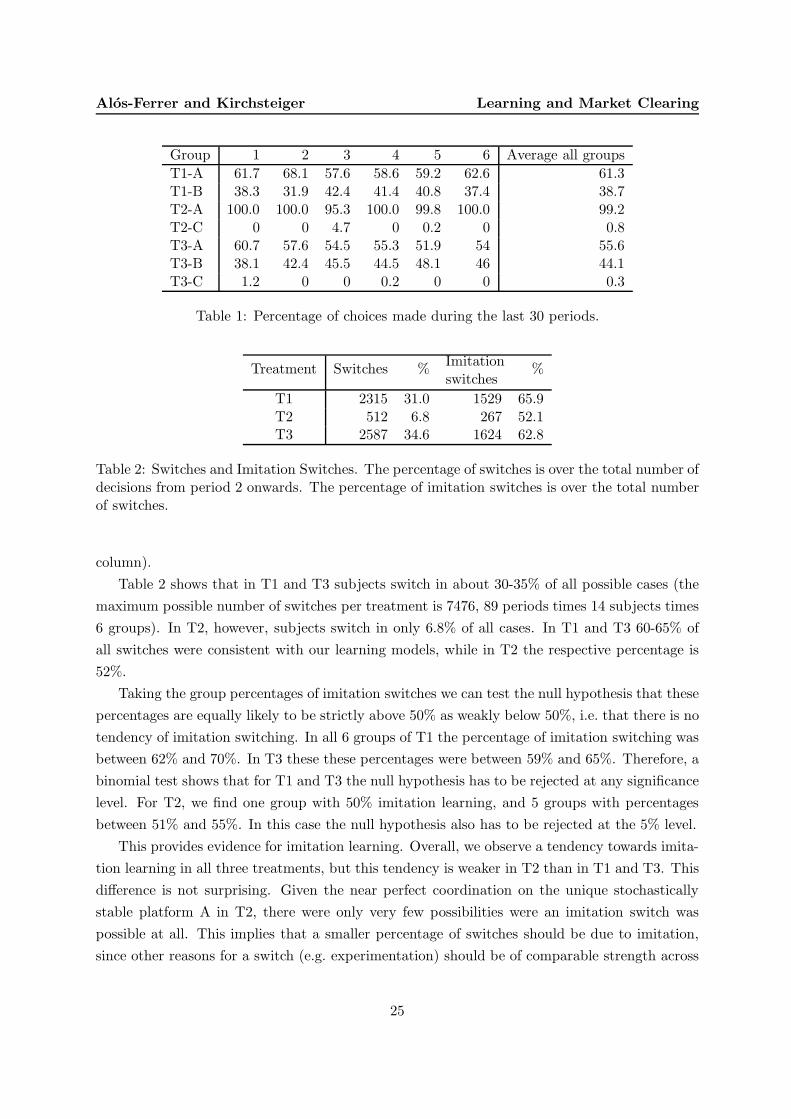
observed for each individual group. Table 1 presents, for all individual groups, the percentage
23

Alos-Ferrer and Kirchsteiger Learning and Market Clearing
Figure 3: Evolution of the number of traders in each institution in T3 (averaged across sixsessions).
of traders opting for the different feasible platforms during the last 30 periods. For example, in
group 2 of T3 57.6% of the traders opted for platform A during the last 30 rounds, 42.4% for
platform B, and 0% for platform C.
In all groups at least 50% of the traders opted for platform A during the last 30 periods. If
available, at least 30% opted for platform B. But less than 5% opted for platform C, and in 10
out of 12 cases less than 1 percent of the traders opted for C when available.
Overall, this result gives a strong support for the main predictions of the theoretical model,
namely that market clearing as well as other stochastically stable institutions will be used in
the long run, while other institutions will be avoided. To further investigate the reasons for this
result, we take a closer look at the individual behavior. In particular, we investigate the behavior
of traders who change the platform from one period to the next (“platform switching”).
In Table 2 we provide the number of switches observed for the different treatments as absolute
numbers and as percentage of the number of total decisions. We also look at the number of
cases where subjects switch to an institution which gave the traders of their own type the highest
possible payoff in the last period, i.e. switches consistent with our model (fourth column). Since
in these cases the subjects imitate the most successful last period choice, we call them imitation
switches. Table 2 also provides the percentage of imitation switches over all switches (fifth
24
Alos-Ferrer and Kirchsteiger Learning and Market Clearing
Group 1 2 3 4 5 6 Average all groups
T1-A 61.7 68.1 57.6 58.6 59.2 62.6 61.3T1-B 38.3 31.9 42.4 41.4 40.8 37.4 38.7T2-A 100.0 100.0 95.3 100.0 99.8 100.0 99.2T2-C 0 0 4.7 0 0.2 0 0.8T3-A 60.7 57.6 54.5 55.3 51.9 54 55.6T3-B 38.1 42.4 45.5 44.5 48.1 46 44.1T3-C 1.2 0 0 0.2 0 0 0.3
Table 1: Percentage of choices made during the last 30 periods.
Treatment Switches %Imitationswitches
%
T1 2315 31.0 1529 65.9T2 512 6.8 267 52.1T3 2587 34.6 1624 62.8
Table 2: Switches and Imitation Switches. The percentage of switches is over the total number ofdecisions from period 2 onwards. The percentage of imitation switches is over the total numberof switches.
column).
Table 2 shows that in T1 and T3 subjects switch in about 30-35% of all possible cases (the
maximum possible number of switches per treatment is 7476, 89 periods times 14 subjects times
6 groups). In T2, however, subjects switch in only 6.8% of all cases. In T1 and T3 60-65% of
all switches were consistent with our learning models, while in T2 the respective percentage is
52%.
Taking the group percentages of imitation switches we can test the null hypothesis that these
percentages are equally likely to be strictly above 50% as weakly below 50%, i.e. that there is no
tendency of imitation switching. In all 6 groups of T1 the percentage of imitation switching was
between 62% and 70%. In T3 these these percentages were between 59% and 65%. Therefore, a
binomial test shows that for T1 and T3 the null hypothesis has to be rejected at any significance
level. For T2, we find one group with 50% imitation learning, and 5 groups with percentages
between 51% and 55%. In this case the null hypothesis also has to be rejected at the 5% level.
This provides evidence for imitation learning. Overall, we observe a tendency towards imita-
tion learning in all three treatments, but this tendency is weaker in T2 than in T1 and T3. This
difference is not surprising. Given the near perfect coordination on the unique stochastically
stable platform A in T2, there were only very few possibilities were an imitation switch was
possible at all. This implies that a smaller percentage of switches should be due to imitation,
since other reasons for a switch (e.g. experimentation) should be of comparable strength across
25

Alos-Ferrer and Kirchsteiger Learning and Market Clearing
all treatments. In summary:
Result 2: Individual traders tend to switch to a platform which in the last period gave the
highest payoff to traders of their own type. This tendency is stronger in T1 and T3 than in T2.
To further investigate individual behavior, the learning model must be further specified. In
particular, as mentioned in Section 3.3, we hypothesized that the likelihood of a revision would
depend on the observed payoff differences between the own and other institutions. Hence, we test
a learning model where the revision probability is strictly increasing in the difference between
the highest last-period-own-type payoff and the last-period-own payoff.
Denote by ∆ the difference between the highest last-period-own-type payoff and the last-
period-own payoff. For the case of two platforms, s denotes a dummy which simply takes value
1 if a switch to the other platform occurs. For T3, the definition of s is more involved, because
many more possibilities exist. We define s as a variable which takes the value 1 if either last
period’s platform did not deliver maximal payoffs and a switch to the last-period-best among
the other two platforms occurred, or last-period’s platform did deliver maximal payoffs and a
switch to some other platform occurred. This definition is the natural generalization of the
dummy variable for the two platform case. The logic is as follows. Consider first the case where
∆ > 0, that is, last period’s platform did not deliver the highest payoffs. In the two-platform
case, the decision consistent with our basic decision rule involves a switch, i.e. s = 1. In the
three-platform case, s = 1 indicates again the choice consistent with the basic decision rule,
which corresponds to a switch to the appropriate platform, but not to the third one. In the case
∆ = 0, the decision consistent with our basic decision rule in the two-platform case is to stay,
i.e. s = 0. In the three-platform case, s = 0 again indicates the choice consistent with the basic
decision rule. The main difference between the dummy variables in the two- and three-platform
cases is that, when ∆ > 0, with three platforms a value of s = 0 might indicate either that the
agent did stay in his previous platform (which might correspond to either inertia or a mistake),
or also to a switch to a “third platform”, which is neither his previous one nor the one which
delivered highest payoffs. Switches of the last type can obviously not occur in the two-platform
case. But in T3 only 85 decisions (out of 7476) were of this type.
Since each trader has to decide 89 times whether to switch or not, we have a strongly balanced
panel data set. We conduct a probit regression with random effects with s as dependent variable.
The most important independent variable is ∆, and to allow for nonlinearities, we include ∆2.
We also include the period, a type dummy, and dummies for the groups. Since all group dummies
are insignificant except for one group in T3, they are not reported in Table 3.
The regressions deliver the following main result.
Result 3: In all three treatments, the switching probability is strictly increasing in the difference
between highest last-period-own-type payoff and the last-period-own payoff.
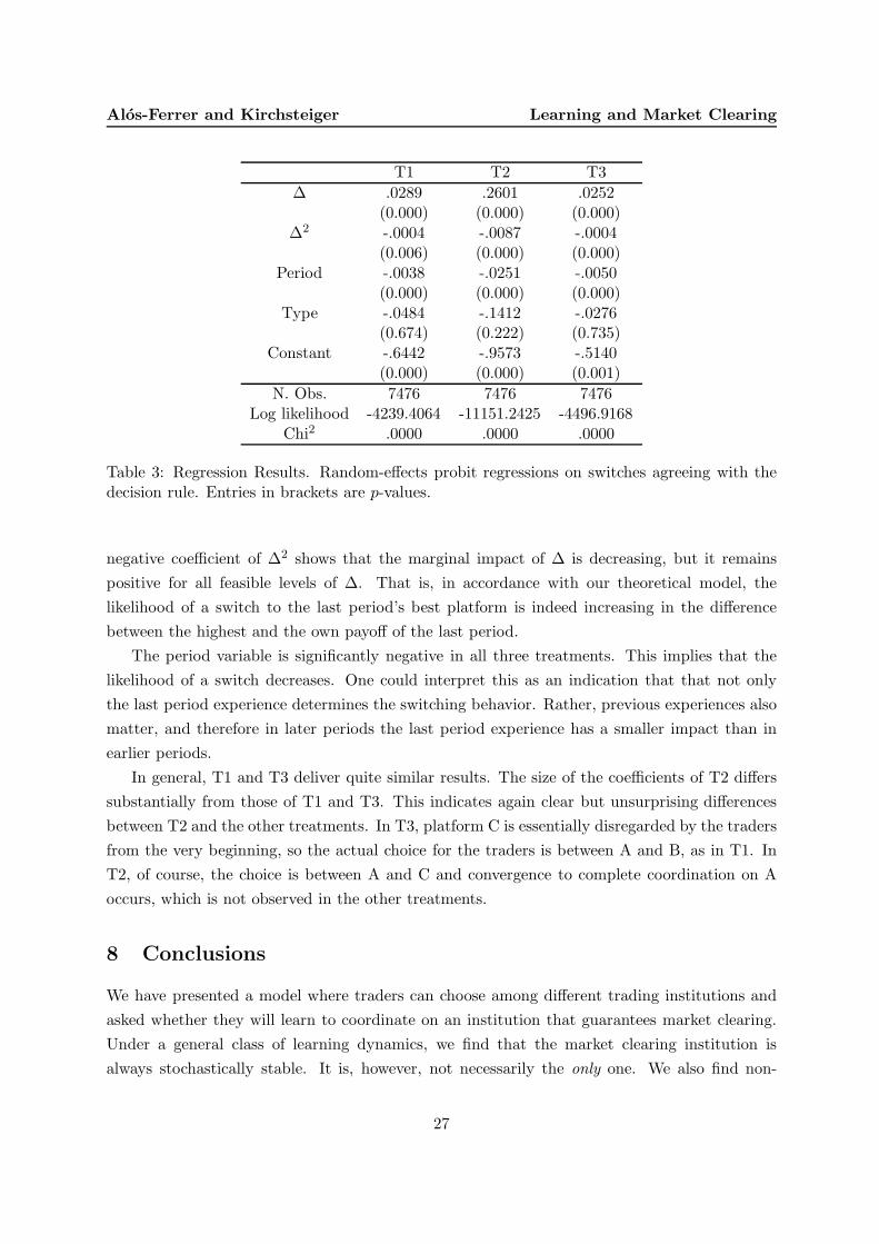
As can be seen from Table 3, in all three treatments the impact of ∆ on s is positive and
highly significant (p-values are shown in brackets below the corresponding coefficients). The
26
Alos-Ferrer and Kirchsteiger Learning and Market Clearing
T1 T2 T3
∆ .0289 .2601 .0252(0.000) (0.000) (0.000)
∆2 -.0004 -.0087 -.0004(0.006) (0.000) (0.000)
Period -.0038 -.0251 -.0050(0.000) (0.000) (0.000)
Type -.0484 -.1412 -.0276(0.674) (0.222) (0.735)
Constant -.6442 -.9573 -.5140(0.000) (0.000) (0.001)
N. Obs. 7476 7476 7476Log likelihood -4239.4064 -11151.2425 -4496.9168
Chi2 .0000 .0000 .0000
Table 3: Regression Results. Random-effects probit regressions on switches agreeing with thedecision rule. Entries in brackets are p-values.
negative coefficient of ∆2 shows that the marginal impact of ∆ is decreasing, but it remains
positive for all feasible levels of ∆. That is, in accordance with our theoretical model, the
likelihood of a switch to the last period’s best platform is indeed increasing in the difference
between the highest and the own payoff of the last period.
The period variable is significantly negative in all three treatments. This implies that the
likelihood of a switch decreases. One could interpret this as an indication that that not only
the last period experience determines the switching behavior. Rather, previous experiences also
matter, and therefore in later periods the last period experience has a smaller impact than in
earlier periods.
In general, T1 and T3 deliver quite similar results. The size of the coefficients of T2 differs
substantially from those of T1 and T3. This indicates again clear but unsurprising differences
between T2 and the other treatments. In T3, platform C is essentially disregarded by the traders
from the very beginning, so the actual choice for the traders is between A and B, as in T1. In
T2, of course, the choice is between A and C and convergence to complete coordination on A
occurs, which is not observed in the other treatments.
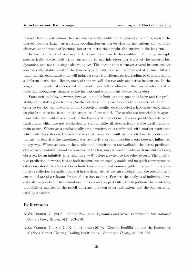
8 Conclusions
We have presented a model where traders can choose among different trading institutions and
asked whether they will learn to coordinate on an institution that guarantees market clearing.
Under a general class of learning dynamics, we find that the market clearing institution is
always stochastically stable. It is, however, not necessarily the only one. We also find non-
27
Alos-Ferrer and Kirchsteiger Learning and Market Clearing
market clearing institutions that are stochastically stable under general conditions, even if the
market becomes large. As a result, coordination on market-clearing institutions will be often
observed as the result of learning, but other institutions might also survive in the long run.
In the framework of our model, this conclusion has to be qualified. Formally, multiple
stochastically stable institutions correspond to multiple absorbing states of the unperturbed
dynamics, and not to a single absorbing set. This means that whenever several institutions are
stochastically stable, most of the time only one institution will be observed at a time. After a
time, though, experimentation will induce a short transitional period leading to coordination in
a different institution. Hence, most of time we will observe only one active institution. In the
long run, different institutions with different prices will be observed; this can be interpreted as
reflecting endogenous changes in the institutional environment favored by traders.
Stochastic stability, however, involves a double limit as time goes to infinity and the prob-
ability of mistakes goes to zero. Neither of these limits corresponds to a realistic situation. In
order to test for the relevance of our theoretical results, we conducted a laboratory experiment
on platform selection based on the structure of our model. The results are remarkably in agree-
ment with the qualitative content of the theoretical predictions. Traders quickly learn to avoid
institutions which are not stochastically stable, while all stochastically stable institutions re-
main active. Whenever a stochastically stable institution is confronted with another institution
which fails this criterion, the outcome is a sharp selection result, as predicted by the model, even
though the length of the experiment was relatively short and decision errors were not influenced
in any way. Whenever two stochastically stable institutions are available, the literal prediction
of stochastic stability cannot be observed in the lab, since it would involve each institution being
observed for an infinitely long time (as ε → 0) before a switch to the other occurs. The qualita-
tive prediction, however, is that both institutions are equally stable and no quick convergence to
either one should be observed for a finite time interval and non-negligible noise level. This qual-
itative prediction is readily observed in the data. Hence, we can conclude that the predictions of
our model are also relevant for actual decision-making. Further, the analysis of individual-level
data also supports our behavioral assumptions and, in particular, the hypothesis that switching
probabilities increase in the payoff difference between other institutions and the one currently
used by a trader.
References
Alos-Ferrer, C. (2003): “Finite Population Dynamics and Mixed Equilibria,” International
Game Theory Review, 5(3), 263–290.
Alos-Ferrer, C., and G. Kirchsteiger (2010): “General Equilibrium and the Emergence
of (Non) Market Clearing Trading Institutions,” Economic Theory, 44, 339–360.
28

Alos-Ferrer and Kirchsteiger Learning and Market Clearing
Alos-Ferrer, C., G. Kirchsteiger, and M. Walzl (2010): “On the Evolution of Market
Institutions: The Platform Design Paradox,” Economic Journal, 120(543), 215–243.
Alos-Ferrer, C., and N. Netzer (2010): “The Logit-Response Dynamics,” Games and
Economic Behavior, 68, 413–427.
Ariely, D., A. Ockenfels, and A. Roth (2005): “An Experimental Analysis of Ending
Rules in Internet Auctions,” RAND Journal of Economics, 36, 890–907.
Ausubel, L., and P. Cramton (2002): “Demand Reduction and Inefficiency in Multi-Unit
Auctions,” Mimeo.
Bajari, P., and A. Hortacsu (2003): “The Winner’s Curse, Reserve Prices, and Endogenous
Entry: Empirical Insights from eBay Auctions,” RAND Journal of Economics, 34, 329–355.
Benaım, M., and J. Weibull (2003): “Deterministic Approximation of Stochastic Evolution
in Games,” Econometrica, 71, 878–903.
Binmore, K., and L. Samuelson (1997): “Muddling Through: Noisy Equilibrium Selection,”
Journal of Economic Theory, 74, 235–265.
Blume, L. (2003): “How noise matters,” Games and Economic Behavior, 44, 251–271.
Budish, E., and L. Takeyama (2001): “Buy Prices in Online Auctions: Irrationality on the
Internet,” Economics Letters, 72, 325–333.
Ellison, G. (2000): “Basins of Attraction, Long-Run Stochastic Stability, and the Speed of
Step-by-Step Evolution,” Review of Economic Studies, 67, 17–45.
Fudenberg, D., and D. Levine (1998): The Theory of Learning in Games. The MIT Press,
Cambridge, Massachusetts.
Gerber, A., and M. O. Bettzuge (2007): “Evolutionary Choice of Markets,” Economic
Theory, 30, 453–472.
Holt, C. (1995): “Industrial Organization: A Survey of Laboratory Research,” in Handbook of
Experimental Economics, ed. by J. Kagel, and A. Roth. Princeton University Press, Princeton,
NJ.
Ishibuchi, H., C. Oh, and T. Nakashima (2002): “Designing a Decision Making System for
a Market Selection Game,” Mimeo.
Kandori, M., G. J. Mailath, and R. Rob (1993): “Learning, Mutation, and Long Run
Equilibria in Games,” Econometrica, 61, 29–56.
29

Alos-Ferrer and Kirchsteiger Learning and Market Clearing
Kandori, M., and R. Rob (1995): “Evolution of Equilibria in the Long Run: A General
Theory and Applications,” Journal of Economic Theory, 65, 383–414.
Karlin, S., and H. M. Taylor (1975): A First Course in Stochastic Processes, 2nd Ed.
Academic Press, San Diego.
Kugler, T., Z. Neeman, and N. Vulkan (2006): “Markets Versus Negotiations: an Exper-
imental Analysis,” Games and Economic Behavior, 56, 121–134.
Plott, C. (1982): “Industrial Organization Theory and Experimental Economics,” Journal of
Economic Literature, 20, 1485–1587.
Reynolds, S., and J. Wooders (2009): “Auctions with a Buy Price,” Economic Theory, 38,
9–39.
Samuelson, L. (1994): “Stochastic Stability in Games with Alternative Best Replies,” Journal
of Economic Theory, 64, 35–65.
(1997): Evolutionary Games and Equilibrium Selection. The MIT Press, Cambridge,
Massachusetts.
Schlag, K. (1998): “Why Imitate, and if so, how? A Boundedly Rational Approach to Multi-
armed Bandits,” Journal of Economic Theory, 78, 130–156.
Young, P. (1993): “The Evolution of Conventions,” Econometrica, 61, 57–84.
30

Alos-Ferrer and Kirchsteiger Learning and Market Clearing
Appendix A Proofs
Proof of Lemma 1. Suppose βz(nz,mz) < 1. Then buyers, but not sellers, are rationed at
institution z. We have that q0S = s(p0) and qzS = s(pz). Suppose now that vS(q0S, p0) ≤ vS(q
zS , pz).
By A1, we must have that p0 ≤ pz.
Then, again by A1, vB(q0B , p0) ≥ vB(d(pz), pz). Since d(pz) > qzB (buyers are rationed), A2
implies that vB(d(pz), pz) > vB(qzB , pz).
The case βz(nz,mz) > 1 is analogous.
If βz(nz,mz) = 1, no traders are rationed, and the analogous arguments follow with weak
inequalities (A2 does not apply since there is no rationing).
We now prove some auxiliary lemmata. The first shows that traders in an inactive institution
will always prefer any active institution.
Lemma 2. Suppose institution z is inactive and institution z′ is active. If traded quantities are
not zero at z′, any trader in z or z′ strictly prefers the outcome of institution z′ to that of z. If
traded quantities are zero at z′, traders in z or z′ are indifferent between the two institutions.
Proof. Since mz = 0 or nz = 0, traded quantities are zero at z. Since both the bias βz′(nz′ ,mz′)
and the market-clearing price p∗(nz′ ,mz′) are strictly positive, it follows that pz′(nz′ ,mz′) > 0.
If d (pz′(nz′ ,mz′)) > 0, the claim then follows from assumption A3. If d (pz′(nz′ ,mz′)) = 0, the
claim follows from our explicit assumption as part of A3 that evaluations do not depend on
hypothetical prices.
Lemma 3. Assume A1-A3. Under D0-D2, given any state ω with n0 (ω) ≥ 1 and m0 (ω) ≥ 1,
there exists a finite, positive probability path of the unperturbed dynamics leading from ω to the
state ω0 with n0 (ω0) = n and m0 (ω0) = m.
Proof. Consider any institution z 6= 0, which is chosen by some traders in state ω. If nz (ω) = 0
or mz (ω) = 0, by Lemma 2 we can build a positive probability path to a new state where
no trader is at institution z. Hence, without loss of generality, suppose nz = nz (ω) > 0 and
mz = mz (ω) > 0.
If βz(nz,mz) 6= 1, it follows from Lemma 1 that in state ω at least one of the two types of
traders strictly prefers the market clearing institution. Let k be a trader of that type who is
at the non-market clearing institution z. It might happen that k prefers a third institution to
the market clearing one, but certainly will not stay in z if given revision opportunity. Further,
by Assumption D1, there is strictly positive probability that k is the only trader of his type
obtaining revision opportunity. Consider the paths where this event happens, and let k′ denote a
trader of the other type (i.e. not of the same type as k) who, in state ω, is in the same non-market
clearing institution z. Consider now the event that only k and k′ get revision opportunity.
31

Alos-Ferrer and Kirchsteiger Learning and Market Clearing
If this event has positive probability, then (if it occurs) k′ may or may not change institution,
but k will, switching to the market clearing or another institution. If the probability of k and
k′ being the only revising traders is zero, by Assumption D2 no agent of the same type as k′
will revise this period, and hence k will change institution but no other agent will. In any case,
the process reaches a state with strictly less traders at institution z than there were in ω, but at
least the same traders in the other institutions (and, in particular, the market clearing one). If
βz(nz,mz) = 1, Lemma 1 yields weak preferences. The argument above applies again, because
by Assumption D0 ties are broken randomly, i.e. if a trader weakly prefers another institution
to his current one, there is a maybe small but positive probability that he switches away.
Repeating this argument, we will reach a state ω′ with either nz (ω′) = 0 or mz (ω
′) = 0.
From this state, all remaining traders will leave institution z as above (by Lemma 2). Hence, we
reach a state where strictly less institutions are chosen than in ω.
Repeating this procedure, we will reach a state where only two institutions are chosen by
traders, and one of them will necessarily be the market clearing one. Applying again the same
argument (using Lemma 1) shows that we can construct a positive probability path to ω0, where
0 is the only active institution.
Lemma 4. Assume A1, A2, and A3. Under D0, D1 and D2,
(i) the absorbing states of the unperturbed dynamics are the “cross-states” ω such that nz (ω) =
n and mz′ (ω) = m for some z, z′ ∈ 0, ..., Z . In particular, this includes all monomorphic
states ωz characterized by nz (ωz) = n and mz (ωz) = m, corresponding to coordination on
a particular institution;
(ii) no state ω with 1 ≤ n0 (ω) ≤ n−1 and 1 ≤ m0 (ω) ≤ m−1 (i.e., where the market clearing
institution is active but not all traders of any type are in it) is part of any absorbing set
of the unperturbed dynamics.
Proof. Cross states as defined in (i) are obviously absorbing because, in the absence of experi-
mentation, traders will never switch to unobserved institutions.13 To see that there are no other
absorbing states, suppose there are traders of the same type in at least two different institutions.
Since necessarily one of those institutions is yielding (weakly) higher payoffs than the other, and
under Assumption D1 there is positive probability that one of the traders not in that institu-
tion is given revision opportunity, there is a positive probability transition to a different state,
a contradiction. Part (ii) follows immediately from Lemma 3.
13Thus, cross-states are absorbing because, if all institutions are inactive, no prices are observed and tradersdo not switch. This is inconsequential. Cross-states are extremely unstable. Specifically, they are destabilizedwith a single mutation, in which one trader joins the traders of the other type. By Lemma 2, the outcome of thenow-active institution is better for all traders than that of the inactive institution. Hence, traders at the inactiveinstitution will switch whenever revision opportunities arise.
32

Alos-Ferrer and Kirchsteiger Learning and Market Clearing
The remaining proofs rely on the characterization of the set of stochastically stable states
introduced by Kandori, Mailath, and Rob (1993) and Young (1993), and in the concept of Radius
and Coradius developed by Ellison (2000). Given two absorbing sets A and B, let c(A,B) > 0
(referred to as the transition cost from A to B) denote the minimal number of mistakes in a
positive probability path starting in an element of A and leading to an element in B. The
following lemma contains all the results on stochastic stability that we require for the analysis.
Its proof is a straightforward application of Ellison (2000, Theorems 1 and 3) and is analogous
to the proof of Lemma 2 in Alos-Ferrer and Kirchsteiger (2010); hence we omit it here.
Lemma 5. Let A be an absorbing set and define the Radius of A by
R(A) = min c(A,B) |B is an absorbing set, B 6= A
and the Coradius of A by
CR(A) = max c(B,A) |B is an absorbing set, B 6= A
Then:
(i) If R(A) ≥ CR(A), the states in A are stochastically stable.
(ii) If R(A) > CR(A), the only stochastically stable states are those in A.
(iii) If the states in an absorbing set B are stochastically stable and R(A) = c(B,A), the states
in A are also stochastically stable.
Proof of Theorem 1. We have to show the stochastic stability of the state ω0. If there is any
other market-clearing institution, the conclusion follows by renaming. First, notice that, by
Lemma 2, no monomorphic state can be left with less than two mutations unless the traded
quantity is zero. Since traded quantities at a market-clearing institution are never zero, it follows
that R(ω0) ≥ 2.
Consider any state in any absorbing set other than ω0. Notice that two mutations (to
the market clearing institution) suffice to reach a state ω with n0 (ω) ≥ 1 and m0 (ω) ≥ 1. By
Lemma 3, there is a positive probability path of the unperturbed dynamics (i.e. requiring no
further mutations) leading to ω0. This shows that CR(ω0) = 2 (the equality follows because
two mutations are required to leave any other monomorphic state). The result follows from
Lemma 5(i).
Proof of Theorem 2. Let ωz denote the monomorphic state corresponding to coordination on
institution z. We know from Theorem 1 that ω0 is stochastically stable. By definition of a
favored institution, we see that if exactly two mutations to institution z occur at state ω0, we
33

Alos-Ferrer and Kirchsteiger Learning and Market Clearing
reach a state where at least one type of traders strictly prefer that institution. Analogously to
the proof of Lemma 3 (through repeated application of Definition 3), from this state there exists
a positive probability path involving no further mutations which leads to state ωz. From the
proof of Theorem 1, we already know that it is possible to make the opposite transition with
exactly two mutations (but no less). Thus, we obtain that c(ω0 , ωz) = 2 = R(ωz), and
the result follows from Lemma 5(iii).
Proof of Theorem 3. For any given n,m, let
R(n,m) =a
b|a = 1, ..., n, and b = 1, ...,m
be the set of feasible buyers-sellers ratios and define
β(n,m) = maxr∈R(n,m)
β(r) and β(n,m) = minr∈R(n,m)
β(r).
Note that for any given number of buyers and sellers, there exists only a finite number of values r
can take. Hence, by A4 β(n,m) < 1 < β(n,m). For any given n,m, define T (n,m) as the set of
all pairs (r0, rz) such that r0 =n0
m0and rz =
nz
mzwith n0, nz ∈ 1, ..., n and m0,mz ∈ 1, ...,m
such that n0 + nz = n and m0 + mz = m. In other words, T (n,m) is the set of all pairs of
buyer-seller ratios which are feasible when exactly two institutions are simultaneously active.
Finally, define
β∗(n,m) = max
β(n,m),max
p(r0)
p(rz)|(r0, rz) ∈ T (n,m) and r0 < rz
β∗(n,m) = min
β(n,m),min
p(r0)
p(rz)|(r0, rz) ∈ T (n,m) and r0 > rz
Notice that β∗(n,m) (and analogously β∗(n,m)) is well-defined because T (n,m) is finite and
r0 < rz implies p(r0)p(rz)
< 1. Clearly, β(n,m) ≤ β∗(n,m) < 1 < β∗(n,m) ≤ β(n,m).
Consider an institution F such that β∗(n,m) < βF (nz,mz) < β∗(n,m) for all feasible nz,mz.
We prove that F is favored.
We want to show that, whenever vS(
q0S, p0)
≥ vS(
qFS , pF)
, then vB(
q0B , p0)
< vB(
qFB , pF)
.
Let βF = βF (nz,mz) be the realized bias at institution F . Suppose βF < 1. Then buyers, but
not sellers, are rationed at F . We have that q0S = s(p0) and qFS = s(pF ). Suppose now that
vS(q0S , p0) ≥ vS(q
FS , pF ). By A1, we must have that p0 ≥ pF .
Suppose r0 ≥ rF . Then, p0 = p(r0) ≥ p(rF ) and, by A1, vB(q0B, p0) = VB(1, r0) ≤ VB(1, rF ).
By A4, VB(1, rF ) < VB(βF , rF ) = vB(
qFB , pF)
and the claim follows.
Suppose now r0 < rF . Then, p0 = p(r0) < p(rF ). If, as assumed, vS(
q0S, p0)
≥ vS(
qFS , pF)
,
then p0 ≥ pF = βF ·p(rF ) by A1. It follows that βF ≤ p(r0)p(rF ) , a contradiction with βF > β∗(n,m).
Hence, vS(
q0S, p0)
< vS(
qFS , pF)
.
34

Alos-Ferrer and Kirchsteiger Learning and Market Clearing
The case βF > 1 is analogous.
The following Lemma is used in the proof of Theorem 4.
Lemma 6. Assume A1 and A4. If β(1) < βB < 1 < βS < β(1), then
(i) if m ≤ n (more buyers than sellers), in a state where an equal, strictly positive number of
sellers and buyers are at an institution z with constant βz = βB and the remaining traders
are at a market-clearing institution (and there are traders of both types in the latter),
buyers strictly prefer z;
(ii) if m ≥ n (more sellers than buyers), in a state where an equal, strictly positive number of
sellers and buyers are at an institution z with constant βz = βS and the remaining traders
are at a market-clearing institution (and there are traders of both types in the latter),
sellers strictly prefer z.
Proof. We will show part (i). Part (ii) is analogous. Let 0 < ℓ < max(m,n) be the number of
sellers and buyers at the alternative institution z. Since m ≤ n, we have that m− ℓ ≤ n− ℓ and
hence
r =n− ℓ
m− ℓ≥ 1
i.e. there are (weakly) more buyers than sellers at the market clearing institution. By A4, since
β(1) < βB < 1,
VB(βB , 1) > VB(1, 1)
and, by A1
VB(1, 1) = vB (qzB(1, 1), p(1)) ≥ vB (d(p(r)), p(r))
because qzB(1, 1) = d(p(1)) and p(1) ≤ p(r) since r ≥ 1 and p is increasing in r. Hence,
VB(βB , 1) > vB (d(p(r)), p(r))
which proves the claim, because vB (d(p(r)), p(r)) is the buyers’ payoff at the market clearing
institution, and VB(βB , 1) is the payoff of the buyers at the non-market clearing institution with
βz = βB .
Proof of Theorem 4. We will show part (i). Part (ii) is analogous. Let ω1 denote the monomor-
phic state corresponding to coordination on the buyers’ institution z. By hypothesis, z is a
favored institution for the economy with K = 1. Further, we know from Theorem 1 that ω0 is
stochastically stable. In order to show stochastic stability of ω1 for large K, by Lemma 5(iii) it
is enough to show that two mutations at ω0 from the market clearing institution 0 to z suffice
for a transition.
35

Alos-Ferrer and Kirchsteiger Learning and Market Clearing
Let a buyer and a seller mutate from 0 to z. Then rz = 1 and r0 = Kn−1Km−1 ≥ 1. By Lemma
6(i), the mutant buyer is strictly better off. By D3K , let K buyers revise, including the mutant,
and follow him to z (so exactly K − 1 buyers switch). Now rz =K1 and r0 =
(n−1)KKm−1 .
Since limr→∞ p(r) = +∞ under M1’-M2’, rz → ∞ as K → ∞, and r0 → n−1m
(finite),
even though βz < 1 it follows that there exists K∗ such that, for all K ≥ K∗, pz = βzp∗(rz) >
p∗(r0) = p0.
Sellers are not rationed at 0 (by definition) and they are not rationed at z either since βz < 1.
Hence by A1 sellers are strictly better off at z since they face a higher price. By D3K , there
is positive probability that K sellers, including the lone seller already in z, revise and move
to z from 0, while no other trader receives revision opportunity. In the new state, we have
rz = KK
= 1 and r0 = (n−1)K(m−1)K = (n−1)
(m−1) . By Lemma 6(i), VB(βz, rz) > VB(1, r0) and buyers at z
are strictly better off. By D3K , there is positive probability that K buyers from 0 revise and
follow them to z.
We know that the market institution z is favored for the economy with K = 1. That means
that one market side is better off at z for all prices resulting from population proportions which
are feasible in the economy with K = 1 (recall the construction of the set T (m,n) in the proof of
Theorem 3). In the state we have just reached, we have rz = 2KK
= 2 and r0 = (n−2)K(m−1)K = n−2
m−1 ,
which are feasible population proportions in the economy with K = 1.
We conclude that one market side is better off at z. Let K traders of the appropriate market
side switch (using D3K). The new population distribution is always a multiple of K for each
trader type and each institution, hence we can apply the fact that z is favored in the economy
with K = 1 again. Proceeding iteratively, eventually we reach a state where a complete market
side is at institution z. By A3, we can complete the transition by moving groups of K traders
of the other market side to z until the market-clearing institution becomes empty.
Appendix B Experimental Instructions and Payoff Matrices
The instructions and the control questionnaire below are translated from German into English
as literally as possible. These instructions were distributed to type I traders (i.e. sellers) of
treatment T3 (choice between 3 platforms). The instructions for type II traders (buyers) were
symmetric (of course with the appropriate payoffs in the examples). The instructions for T1
and T2 were similar, with the only difference that all the references to choice C were deleted.
Each participant was provided with the appropriate payoff tables for the institutions used in
the experiment. Table 4 displays the payoffs obtained by buyers and sellers at each of the three
institutions used in the experiments. Within each table, each row corresponds to the number n
of buyers present at the institution, each column to the number m of sellers.
36

Alos-Ferrer and Kirchsteiger Learning and Market Clearing
Instructions - Type I
The experiment you are about to participate in is part of a research project on decision
behavior. The instructions are simple, and if you read them carefully and make appropriate
decisions, you can earn a considerable amount of money.
The revenues made during the experiment are counted in ECU (“experimental currency
units”). After the end of the experiment all the revenues you made during the experiment will
be added up and paid to you in cash. For every ECU you will receive 0.7 Eurocent.
Any communication between the participants is strictly forbidden.
In every round of the experiment you have to choose between three different options, A, B,
or C. To do so you click on the appropriate button for decision A, B, or C. Then you confirm
your decision by clicking on the OK button. In each round you have half a minute to make this
decision.
In this experiment there are two types of participants, participants of Type I and participants
of Type II. You are of Type I. All in all, there are 7 participants of Type I and 7 participants of
Type II within the group relevant for you. You will not be informed about the identity of the
other group members, and the other group members will not be informed about your identity.
The revenues you make in a round depend on the number of other group members of each
type who make the same decision as you. Assume that you have made decision A, three other
Type I participants have made the same decision, and 5 Type II participants have chosen A,
too. In this case 4 Type I participants and 5 Type II participants have chosen A. As you can
see from the attached revenue matrix, your revenues are 21 ECU in this case.
Another example: You have chosen B, one other Type I participant has made the same
decision, and 3 Type II participants have chosen B, too. In this case your revenues are 20 ECU.
After all members of your group have made a decision, you will be informed about the number
of participants of each type that have chosen A, B, and C. You will also be informed about their
revenues, and about the sum of revenues you have earned so far in the whole experiment.
After that, a new round will start, in which you will have to decide between A, B, and C,
again. Overall there will be 90 rounds.
Control Questionnaire.
1. Suppose that you have made decision B, 2 other Type I participants have made the same
decision, and 2 Type II participants have also chosen B. What are your revenues?
Suppose that 2 Type I participants and 3 Type II participants have chosen A. What are
the revenues of those Type I participants who have chosen A?
Suppose the remaining 2 Type I participants and the remaining 2 Type II participants
have chosen C. What are the revenues of those Type I participants who have chosen C?
37
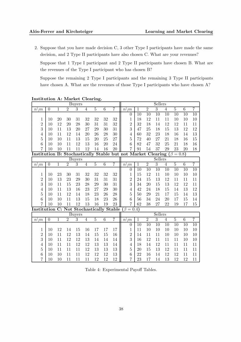
Alos-Ferrer and Kirchsteiger Learning and Market Clearing
2. Suppose that you have made decision C, 3 other Type I participants have made the same
decision, and 2 Type II participants have also chosen C. What are your revenues?
Suppose that 1 Type I participant and 2 Type II participants have chosen B. What are
the revenues of the Type I participant who has chosen B?
Suppose the remaining 2 Type I participants and the remaining 3 Type II participants
have chosen A. What are the revenues of those Type I participants who have chosen A?
Institution A: Market Clearing.Buyers Sellers
n\m 0 1 2 3 4 5 6 7 n\m 1 2 3 4 5 6 70 10 10 10 10 10 10 10
1 10 20 30 31 32 32 32 32 1 18 12 11 11 10 10 102 10 12 20 28 30 31 31 32 2 32 18 14 12 12 11 113 10 11 13 20 27 29 30 31 3 47 25 18 15 13 12 124 10 11 12 14 20 26 28 30 4 60 32 23 18 16 14 135 10 10 11 13 15 20 25 27 5 72 40 27 21 18 16 156 10 10 11 12 13 16 20 24 6 82 47 32 25 21 18 167 10 10 11 11 12 14 16 20 7 91 54 37 29 23 20 18
Institution B: Stochastically Stable but not Market Clearing (β = 0.8)Buyers Sellers
n\m 0 1 2 3 4 5 6 7 n\m 1 2 3 4 5 6 70 10 10 10 10 10 10 10
1 10 23 30 31 32 32 32 32 1 15 12 11 10 10 10 102 10 13 23 29 30 31 31 31 2 24 15 13 12 11 11 113 10 11 15 23 28 29 30 31 3 34 20 15 13 12 12 114 10 11 13 16 23 27 29 30 4 42 24 18 15 14 13 125 10 11 12 14 18 23 26 28 5 50 29 21 17 15 14 136 10 10 11 13 15 18 23 26 6 56 34 24 20 17 15 147 10 10 11 12 13 16 19 23 7 62 38 27 22 19 17 15
Institution C: Not Stochastically Stable (β = 0.4)Buyers Sellers
n\m 0 1 2 3 4 5 6 7 n\m 1 2 3 4 5 6 70 10 10 10 10 10 10 10
1 10 12 14 15 16 17 17 17 1 11 10 10 10 10 10 102 10 11 12 13 14 15 15 16 2 14 11 11 10 10 10 103 10 11 12 12 13 14 14 14 3 16 12 11 11 11 10 104 10 11 11 12 12 13 13 14 4 18 14 12 11 11 11 115 10 11 11 11 12 13 13 13 5 20 15 13 12 11 11 116 10 10 11 11 12 12 12 13 6 22 16 14 12 12 11 117 10 10 11 11 11 12 12 12 7 23 17 14 13 12 12 11
Table 4: Experimental Payoff Tables.
38


![FUEL INJECTION TIMINGS OF A DIRECT INJECTION DIESEL …ijame.ump.edu.my/images/Volume_11 June 2015/16...investigated theoretically and experimentally [18] with fuel injection timing](https://img.pdfslide.net/doc/110x75/5e82db816a24dd167f652436/fuel-injection-timings-of-a-direct-injection-diesel-ijameumpedumyimagesvolume11.jpg)
![Nematic Ordering in Mixtures of Polymers and Liquid Crystalslabo.bio.kyutech.ac.jp/~matuyama/_src/4856/kiyou02.pdf · both experimentally[2-8] and theoretically[8-14]. In contrast,](https://img.pdfslide.net/doc/110x75/5f1f23b0faf940590603b503/nematic-ordering-in-mixtures-of-polymers-and-liquid-matuyamasrc4856kiyou02pdf.jpg)

![JOURNAL OF QUANTUM ELECTRONICS 1 Bistable beam ......by us in liquid crystals without external feedback [36]. In this Paper we address, both experimentally and theoretically, OB between](https://img.pdfslide.net/doc/110x75/60f8f18134b3dd4ff07bd661/journal-of-quantum-electronics-1-bistable-beam-by-us-in-liquid-crystals.jpg)


![Selective adsorption of carbon dioxide from mixed vapors by ......carbon, activated carbon, silicalite, C 186 schwarzite, and nanoporous carbon experimentally or theoretically [1 –9]](https://img.pdfslide.net/doc/110x75/60f7907564e7b45e607c574a/selective-adsorption-of-carbon-dioxide-from-mixed-vapors-by-carbon-activated.jpg)


![#3] Giant Magnetoresistance: Experimentally Driven 1986-1989; Theoretically Modeled 1989; IT Applications into 1990’s First Commerical Hard-Disks with](https://img.pdfslide.net/doc/110x75/56649d925503460f94a79639/3-giant-magnetoresistance-experimentally-driven-1986-1989-theoretically.jpg)