Least Squares Conformal Mapsfor Automatic Texture Atlas Generation

Bruno Lévy Sylvain Petitjean Nicolas Ray Jérome Maillot∗

ISA (Inria Lorraine and CNRS), France

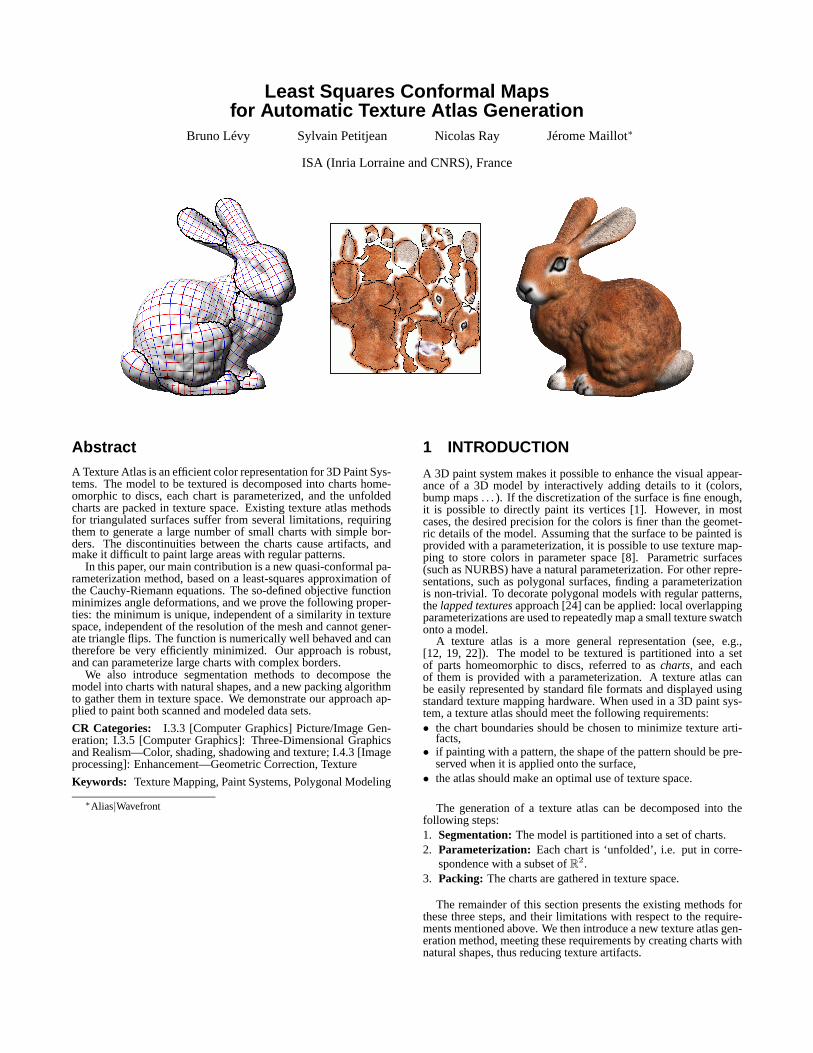
AbstractA Texture Atlas is an efficient color representation for 3D Paint Sys-tems. The model to be textured is decomposed into charts home-omorphic to discs, each chart is parameterized, and the unfoldedcharts are packed in texture space. Existing texture atlas methodsfor triangulated surfaces suffer from several limitations, requiringthem to generate a large number of small charts with simple bor-ders. The discontinuities between the charts cause artifacts, andmake it difficult to paint large areas with regular patterns.

In this paper, our main contribution is a new quasi-conformal pa-rameterization method, based on a least-squares approximation ofthe Cauchy-Riemann equations. The so-defined objective functionminimizes angle deformations, and we prove the following proper-ties: the minimum is unique, independent of a similarity in texturespace, independent of the resolution of the mesh and cannot gener-ate triangle flips. The function is numerically well behaved and cantherefore be very efficiently minimized. Our approach is robust,and can parameterize large charts with complex borders.

We also introduce segmentation methods to decompose themodel into charts with natural shapes, and a new packing algorithmto gather them in texture space. We demonstrate our approach ap-plied to paint both scanned and modeled data sets.

CR Categories: I.3.3 [Computer Graphics] Picture/Image Gen-eration; I.3.5 [Computer Graphics]: Three-Dimensional Graphicsand Realism—Color, shading, shadowing and texture; I.4.3 [Imageprocessing]: Enhancement—Geometric Correction, Texture

Keywords: Texture Mapping, Paint Systems, Polygonal Modeling

∗Alias|Wavefront

1 INTRODUCTION

A 3D paint system makes it possible to enhance the visual appear-ance of a 3D model by interactively adding details to it (colors,bump maps . . . ). If the discretization of the surface is fine enough,it is possible to directly paint its vertices [1]. However, in mostcases, the desired precision for the colors is finer than the geomet-ric details of the model. Assuming that the surface to be painted isprovided with a parameterization, it is possible to use texture map-ping to store colors in parameter space [8]. Parametric surfaces(such as NURBS) have a natural parameterization. For other repre-sentations, such as polygonal surfaces, finding a parameterizationis non-trivial. To decorate polygonal models with regular patterns,thelapped texturesapproach [24] can be applied: local overlappingparameterizations are used to repeatedly map a small texture swatchonto a model.

A texture atlas is a more general representation (see, e.g.,[12, 19, 22]). The model to be textured is partitioned into a setof parts homeomorphic to discs, referred to ascharts, and eachof them is provided with a parameterization. A texture atlas canbe easily represented by standard file formats and displayed usingstandard texture mapping hardware. When used in a 3D paint sys-tem, a texture atlas should meet the following requirements:• the chart boundaries should be chosen to minimize texture arti-

facts,• if painting with a pattern, the shape of the pattern should be pre-

served when it is applied onto the surface,• the atlas should make an optimal use of texture space.

The generation of a texture atlas can be decomposed into thefollowing steps:1. Segmentation:The model is partitioned into a set of charts.2. Parameterization: Each chart is ‘unfolded’, i.e. put in corre-

spondence with a subset ofR2.3. Packing: The charts are gathered in texture space.

The remainder of this section presents the existing methods forthese three steps, and their limitations with respect to the require-ments mentioned above. We then introduce a new texture atlas gen-eration method, meeting these requirements by creating charts withnatural shapes, thus reducing texture artifacts.

1.1 Previous Work

Segmentation into charts. In [13] and [22], the model is interac-tively partitioned by the user. To perform automatic segmentation,Maillot et al. [19] group the facets by their normals. Several multi-resolution methods [6, 15] decompose the model into charts corre-sponding to the simplices of the base complex. In [25], Sanderetal. use a region-growing approach to segmentation, merging chartsaccording to both planarity and compactness criteria. All these ap-proaches are designed to produce charts that can be treated by ex-isting parameterization methods, which are limited to small chartswith simple borders. For this reason, a large number of charts isgenerated, which introduces many discontinuities when construct-ing a texture atlas.

Chart parameterization. The theory of graph embedding hasbeen used by several authors to design parameterization methods.An approximation of Harmonic Maps [4] has been described byEck et al. in [3]. However, the approximation may cause triangleflips. Barycentric Maps [28] offer better guarantees, and have beenused in [5] and in [17]. The method proposed in [25] uses a met-ric minimizing both distortions and texture deviations when used totexture map different levels of details. All the methods mentionedabove require the border of the charts to be fixed on a convex poly-gon in parameter space, which therefore requires to decompose themodel into a large number of charts.

The non-linear MIPS method [9] overcomes this limitation bymaking it possible to extrapolate the parameterization. The borderof the chart can then reach a natural shape in parameter space. How-ever, it requires a time-consuming non-linear optimization. More-over, the non-linear function may present local minima in which thesolver can get stuck. Other methods [16, 23, 29] can also extrap-olate the border, but do not guarantee the absence of triangle flipsand require interaction with the user.

Riemann’s theory on Conformal Maps describes angle-preserving parameterizations. Hakeret al. [7] propose such amethod in the specific case of a surface triangulation homeomor-phic to a sphere. In [11], Hurdalet al. propose a method to flattenmodels of human brains based oncircle packings, which are certainconfigurations of circles with specified pattern of tangencies knownto provide a way to approximate the Riemann mapping. Buildingcircle packings is however quite expensive. The approach proposedin [26] consists in solving for the angles in parameter space. It re-sults in a highly constrained optimization problem. We introducehere a conformal mapping method, offering more guarantees, effi-ciency and robustness than those approaches.

Charts packing in texture space. Finding the optimal packingof the charts in texture space is a computational geometry problemknown asbin packing. It has been studied by several authors, suchas Milenkovic (see, e.g., [20]), but the resulting algorithms take ahuge amount of time since the problem is NP-complete. To speedup these computations, several heuristics have been proposed in thecomputer graphics community. In the case of individual triangles,such a method is described by several authors (see, e.g., [2]). Inthe general case of charts, Sanderet al. [25] propose an approachto pack the minimal area bounding rectangles of the charts. In ourcase, since we generate a small number of large charts rather than alarge number of small charts as in classical approaches, the chartscan have complex borders, and the bounding rectangle can be faraway from the boundary of the charts. Therefore, a lot of texturespace can be wasted. For this reason, we propose a more accuratepacking algorithm that can handle the complex charts created byour segmentation and parameterization methods.

1.2 Overview

The paper is organized as follows. Since it is our main contribu-tion, we will start by introducing Least Squares Conformal Maps(LSCMs), a new optimization-based parameterization method withthe following properties (see Section 2 and Figure1):• Our criterionminimizes angle deformations and non-uniform

scaling. It can be efficiently minimized by classical NA methods,and does not require a complex algorithm such as the ones usedin [11] and in [26].

• We prove theexistence and uniqueness of the minimumofthis criterion. Therefore, the solver cannot get stuck in a localminimum, in contrast with non-linear methods [9, 23, 25, 29]where this property is not guaranteed.

• The borders of the charts do not need to be fixed, as with mostof the existing methods [3, 5, 17]. Therefore,large charts witharbitrarily shaped borders can be parameterized.

• We prove that the orientation of the triangles is preserved, whichmeans thatno triangle flip can occur. However, as in [26], over-laps may appear, when the boundary of the surface self-intersectsin texture space. Such configurations are automatically detected,and the concerned charts are subdivided. This problem was sel-dom encountered in our experiments.

• We prove that the result isindependent of the resolution of themesh, which means that LSCMs can be used to parameterizeLODs and irregularly sampled objects without introducing anytexture deviation. To ensure this property, it is not necessary toadd a non-linear term in the criterion, such as the one proposedin [25].

In Section 3, we present a new segmentation method to decom-pose the model into charts. Thanks to the additional flexibility of-fered by LSCMs, it is possible to create large charts correspond-ing to meaningful geometric entities, such as biological features ofcharacters and animals. The required number of charts is dramati-cally reduced, together with the artifacts caused by the discontinu-ities between the charts. Moreover, these large charts facilitate theuse of regular patterns in a 3D paint system.

Section 4 presents our method to pack the charts in texture space.Since our segmentation method can create charts with complex bor-ders, we pack the charts more accurately than with bounding rect-angles, as in previous approaches. Our method is inspired by thestrategy used by a ‘Tetris’ player. The paper concludes with someresults, on both scanned and modeled meshes.

2 LEAST SQUARES CONFORMAL MAPS

In this section, we focus on the problem of parameterizing a charthomeomorphic to a disc. It will then be shown how to decomposethe model into a set of charts, and how to pack these charts in texturespace.

2.1 Notations

• scalars are denoted by normal charactersx, y, u, v,• vectors are denoted by bold charactersx = (x, y),• complex numbers are denoted by capitalsU = (u+ iv),• vectors of complex numbers are denoted by bold capitalsU,• maps and matrices are denoted by cursive fontsU , X .

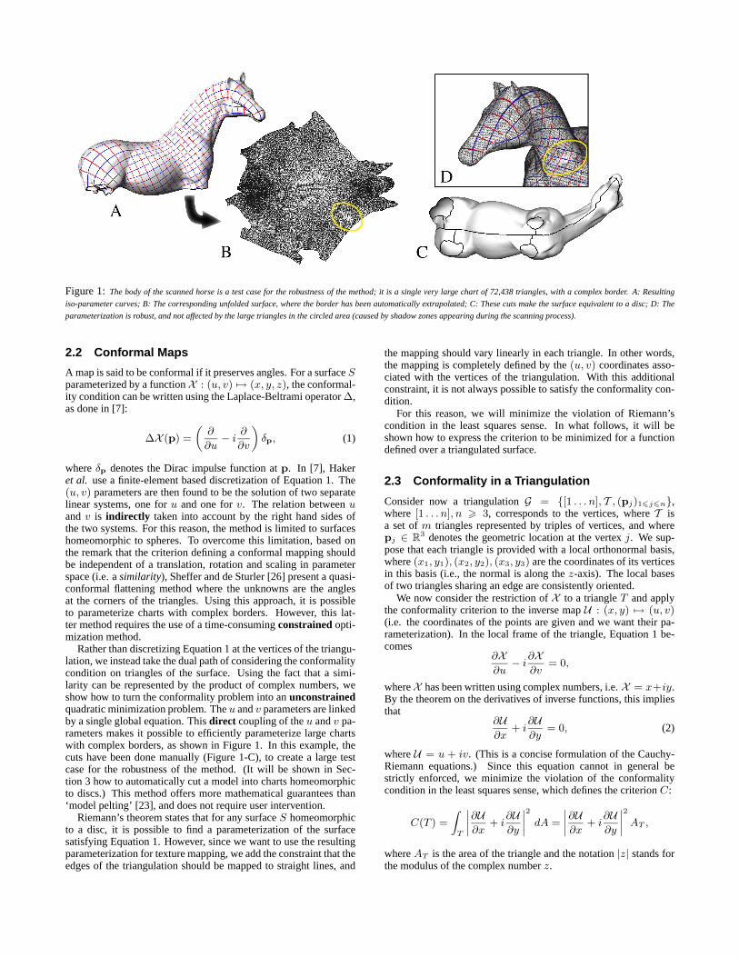
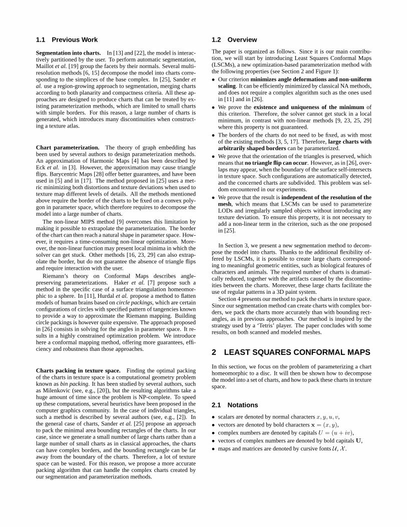
Figure 1: The body of the scanned horse is a test case for the robustness of the method; it is a single very large chart of 72,438 triangles, with a complex border. A: Resulting

iso-parameter curves; B: The corresponding unfolded surface, where the border has been automatically extrapolated; C: These cuts make the surface equivalent to a disc; D: The

parameterization is robust, and not affected by the large triangles in the circled area (caused by shadow zones appearing during the scanning process).

2.2 Conformal Maps

A map is said to be conformal if it preserves angles. For a surfaceSparameterized by a functionX : (u, v) 7→ (x, y, z), the conformal-ity condition can be written using the Laplace-Beltrami operator∆,as done in [7]:

∆X (p) =

(∂

∂u− i ∂

∂v

)δp, (1)

whereδp denotes the Dirac impulse function atp. In [7], Hakeret al. use a finite-element based discretization of Equation1. The(u, v) parameters are then found to be the solution of two separatelinear systems, one foru and one forv. The relation betweenuandv is indirectly taken into account by the right hand sides ofthe two systems. For this reason, the method is limited to surfaceshomeomorphic to spheres. To overcome this limitation, based onthe remark that the criterion defining a conformal mapping shouldbe independent of a translation, rotation and scaling in parameterspace (i.e. asimilarity), Sheffer and de Sturler [26] present a quasi-conformal flattening method where the unknowns are the anglesat the corners of the triangles. Using this approach, it is possibleto parameterize charts with complex borders. However, this lat-ter method requires the use of a time-consumingconstrainedopti-mization method.

Rather than discretizing Equation1 at the vertices of the triangu-lation, we instead take the dual path of considering the conformalitycondition on triangles of the surface. Using the fact that a simi-larity can be represented by the product of complex numbers, weshow how to turn the conformality problem into anunconstrainedquadratic minimization problem. Theu andv parameters are linkedby a single global equation. Thisdirect coupling of theu andv pa-rameters makes it possible to efficiently parameterize large chartswith complex borders, as shown in Figure1. In this example, thecuts have been done manually (Figure1-C), to create a large testcase for the robustness of the method. (It will be shown in Sec-tion 3 how to automatically cut a model into charts homeomorphicto discs.) This method offers more mathematical guarantees than‘model pelting’ [23], and does not require user intervention.

Riemann’s theorem states that for any surfaceS homeomorphicto a disc, it is possible to find a parameterization of the surfacesatisfying Equation1. However, since we want to use the resultingparameterization for texture mapping, we add the constraint that theedges of the triangulation should be mapped to straight lines, and

the mapping should vary linearly in each triangle. In other words,the mapping is completely defined by the(u, v) coordinates asso-ciated with the vertices of the triangulation. With this additionalconstraint, it is not always possible to satisfy the conformality con-dition.

For this reason, we will minimize the violation of Riemann’scondition in the least squares sense. In what follows, it will beshown how to express the criterion to be minimized for a functiondefined over a triangulated surface.

2.3 Conformality in a Triangulation

Consider now a triangulationG = {[1 . . . n], T , (pj)16j6n},where [1 . . . n], n > 3, corresponds to the vertices, whereT isa set ofm triangles represented by triples of vertices, and wherepj ∈ R3 denotes the geometric location at the vertexj. We sup-pose that each triangle is provided with a local orthonormal basis,where(x1, y1), (x2, y2), (x3, y3) are the coordinates of its verticesin this basis (i.e., the normal is along thez-axis). The local basesof two triangles sharing an edge are consistently oriented.

We now consider the restriction ofX to a triangleT and applythe conformality criterion to the inverse mapU : (x, y) 7→ (u, v)(i.e. the coordinates of the points are given and we want their pa-rameterization). In the local frame of the triangle, Equation1 be-comes

∂X∂u− i∂X

∂v= 0,

whereX has been written using complex numbers, i.e.X = x+iy.By the theorem on the derivatives of inverse functions, this impliesthat

∂U∂x

+ i∂U∂y

= 0, (2)

whereU = u + iv. (This is a concise formulation of the Cauchy-Riemann equations.) Since this equation cannot in general bestrictly enforced, we minimize the violation of the conformalitycondition in the least squares sense, which defines the criterionC:

C(T ) =

∫T

∣∣∣∣∂U∂x + i∂U∂y

∣∣∣∣2 dA =

∣∣∣∣∂U∂x + i∂U∂y

∣∣∣∣2 AT ,whereAT is the area of the triangle and the notation|z| stands forthe modulus of the complex numberz.

Summing over the whole triangulation, the criterion to minimizeis then

C(T ) =∑T∈T

C(T ).

2.4 Gradient in a Triangle

Our goal is now to associate with each vertexj a complex num-berUj such that the Cauchy-Riemann equation is satisfied (in theleast squares sense) in each triangle. To this aim, let us rewrite thecriterionC(T ), assuming the mappingU varies linearly inT .

We consider a triangle{(x1, y1), (x2, y2), (x3, y3)} of R2, withscalarsu1, u2, u3 associated with its vertices. We have:(

∂u/∂x

∂u/∂y

)=

1

dT

(y2 − y3 y3 − y1 y1 − y2

x3 − x2 x1 − x3 x2 − x1

)u1

u2

u3

,

wheredT = (x1y2 − y1x2) + (x2y3 − y2x3) + (x3y1 − y3x1) istwice the area of the triangle.

The two components of the gradient can be gathered in a com-plex number:

∂u

∂x+ i

∂u

∂y= − i

dT

(W1 W2 W3

) (u1 u2 u3

)>,

where W1 = (x3 − x2) + i(y3 − y2),W2 = (x1 − x3) + i(y1 − y3),W3 = (x2 − x1) + i(y2 − y1).

The Cauchy-Riemann equation (Equation2) can be rewritten asfollows:

∂U∂x

+ i∂U∂y

= − i

dT

(W1 W2 W3

) (U1 U2 U3

)>= 0,

whereUj = uj + ivj .The objective function thus reduces to

C(U = (U1, . . . , Un)>) =∑T∈T

C(T ), with

C(T ) =1

dT

∣∣∣(Wj1,T Wj2,T Wj3,T ) (Uj1 Uj2 Uj3)>∣∣∣2 ,

where triangleT has vertices indexed byj1, j2, j3. (We have mul-tipliedC(T ) by a factor of 2 to simplify the expression.)

2.5 Least Squares Conformal Maps

C(U) is quadratic in the complex numbersU1, . . . , Un, so can bewritten down as

C(U) = U∗CU, (3)

whereC is a Hermitian symmetricn × n matrix and the notationU∗ stands for the Hermitian (complex) conjugate ofU. C is aninstance of a Hermitian Gram matrix, i.e. it can be written as

C =M∗M,

whereM = (mij) is the sparsem × n matrix (rows are indexedby triangles, columns are indexed by vertices) whose coefficient is

mij =

{Wj,Ti√dTi

if vertex j belongs to triangleTi,

0 otherwise.

For the optimization problem to have a non-trivial solution, someof theUi’s must be set toa priori values. Let us decompose the vec-torU as(U>f ,U

>p )>, whereUf is the vector offreecoordinates of

Figure 2:Our LSCM parameterization is insensitive to the resolution of the mesh.

The iso-parameter curves obtained on a coarse mesh (Figure A) and on a fine one

(Figure B) are identical, and remain stable when the resolution varies within a mesh

(circled zone in Figures C and D).

U (the variables of the optimization problem) andUp is the vectorof pinnedcoordinates ofU, of lengthp (p 6 n). Along the samelines,M can be decomposed in block matrices as

M =(Mf Mp

),

whereMf is am × (n − p) matrix andMp is am × p matrix.Now, Equation3 can be rewritten as

C(U) = U∗M∗MU = ‖MU‖2 = ‖MfUf +MpUp‖2,

where the notation‖v‖2 stands for the inner product< v,v > (vstands for the conjugate ofv).

Rewriting the objective function with only real matrices and vec-tors yields

C(x) = ‖Ax− b‖2 , (4)

with

A =

(M1

f −M2f

M2f M1

f

), b = −

(M1

p −M2p

M2p M1

p

)(U1p

U2p

),

where the superscripts1 and2 stand respectively for the real andimaginary part,‖v‖ stands this time for the traditionalL2-norm of

a vector with real coordinates andx = (U1f>,U2

f>

)> is the vectorof unknowns.

Note thatA is a2m×2(n−p) matrix,b is a vector ofR2m andx is a vector ofR2(n−p) (theui andvi coordinates of the verticesin parameter space that are allowed to move freely).

2.6 Properties

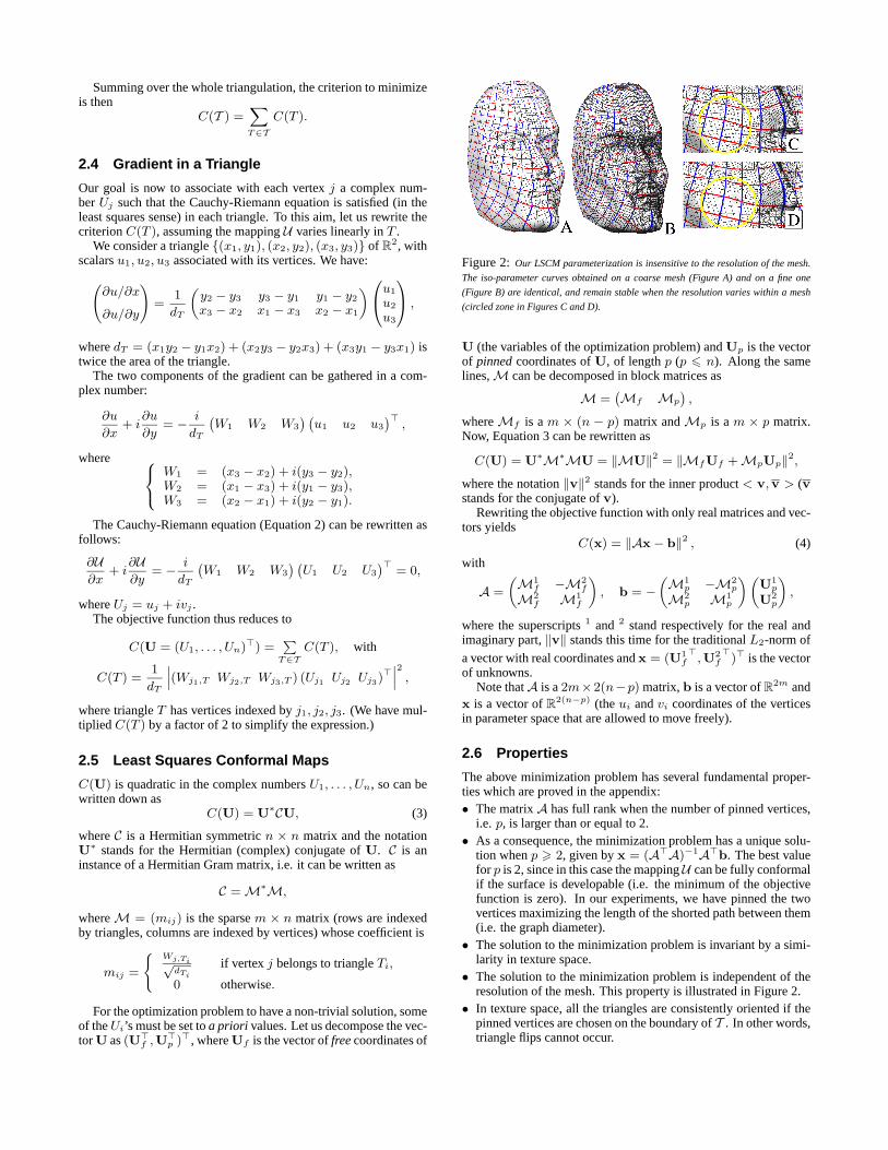
The above minimization problem has several fundamental proper-ties which are proved in the appendix:• The matrixA has full rank when the number of pinned vertices,

i.e. p, is larger than or equal to 2.• As a consequence, the minimization problem has a unique solu-

tion whenp > 2, given byx = (A>A)−1A>b. The best valuefor p is 2, since in this case the mappingU can be fully conformalif the surface is developable (i.e. the minimum of the objectivefunction is zero). In our experiments, we have pinned the twovertices maximizing the length of the shorted path between them(i.e. the graph diameter).

• The solution to the minimization problem is invariant by a simi-larity in texture space.

• The solution to the minimization problem is independent of theresolution of the mesh. This property is illustrated in Figure2.

• In texture space, all the triangles are consistently oriented if thepinned vertices are chosen on the boundary ofT . In other words,triangle flips cannot occur.

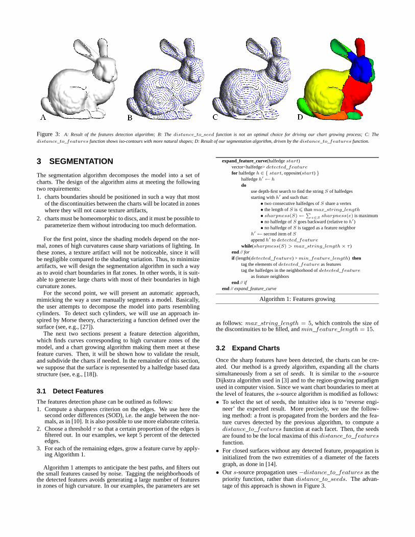
Figure 3: A: Result of the features detection algorithm; B: Thedistance_to_seed function is not an optimal choice for driving our chart growing process; C: The

distance_to_features function shows iso-contours with more natural shapes; D: Result of our segmentation algorithm, driven by thedistance_to_features function.

3 SEGMENTATION

The segmentation algorithm decomposes the model into a set ofcharts. The design of the algorithm aims at meeting the followingtwo requirements:1. charts boundaries should be positioned in such a way that most

of the discontinuities between the charts will be located in zoneswhere they will not cause texture artifacts,

2. charts must be homeomorphic to discs, and it must be possible toparameterize them without introducing too much deformation.

For the first point, since the shading models depend on the nor-mal, zones of high curvatures cause sharp variations of lighting. Inthese zones, a texture artifact will not be noticeable, since it willbe negligible compared to the shading variation. Thus, to minimizeartifacts, we will design the segmentation algorithm in such a wayas to avoid chart boundaries in flat zones. In other words, it is suit-able to generate large charts with most of their boundaries in highcurvature zones.

For the second point, we will present an automatic approach,mimicking the way a user manually segments a model. Basically,the user attempts to decompose the model into parts resemblingcylinders. To detect such cylinders, we will use an approach in-spired by Morse theory, characterizing a function defined over thesurface (see, e.g., [27]).

The next two sections present a feature detection algorithm,which finds curves corresponding to high curvature zones of themodel, and a chart growing algorithm making them meet at thesefeature curves. Then, it will be shown how to validate the result,and subdivide the charts if needed. In the remainder of this section,we suppose that the surface is represented by a halfedge based datastructure (see, e.g., [18]).

3.1 Detect Features

The features detection phase can be outlined as follows:1. Compute a sharpness criterion on the edges. We use here the

second order differences (SOD), i.e. the angle between the nor-mals, as in [10]. It is also possible to use more elaborate criteria.

2. Choose a thresholdτ so that a certain proportion of the edges isfiltered out. In our examples, we kept 5 percent of the detectededges.

3. For each of the remaining edges, grow a feature curve by apply-ing Algorithm 1.

Algorithm 1 attempts to anticipate the best paths, and filters outthe small features caused by noise. Tagging the neighborhoods ofthe detected features avoids generating a large number of featuresin zones of high curvature. In our examples, the parameters are set

expand_feature_curve(halfedgestart)vector<halfedge>detected_featurefor halfedgeh ∈ { start, opposite(start) }

halfedgeh′← h

douse depth-first search to find the stringS of halfedgesstarting withh′ and such that:• two consecutive halfedges ofS share a vertex• the length ofS is6 thanmax_string_length• sharpness(S)←

∑e∈S sharpness(e) is maximum

• no halfedge ofS goes backward (relative toh′)• no halfedge ofS is tagged as a feature neighbor

h′← second item ofSappendh′ to detected_feature

while(sharpness(S) > max_string_length× τ )end // forif (length(detected_feature) >min_feature_length) then

tag the elements ofdetected_feature as featurestag the halfedges in the neighborhood ofdetected_feature

as feature neighborsend // if

end // expand_feature_curve

Algorithm 1: Features growing

as follows:max_string_length = 5, which controls the size ofthe discontinuities to be filled, andmin_feature_length = 15.

3.2 Expand Charts

Once the sharp features have been detected, the charts can be cre-ated. Our method is a greedy algorithm, expanding all the chartssimultaneously from a set ofseeds. It is similar to thes-sourceDijkstra algorithm used in [3] and to the region-growing paradigmused in computer vision. Since we want chart boundaries to meet atthe level of features, thes-source algorithm is modified as follows:• To select the set of seeds, the intuitive idea is to ‘reverse engi-

neer’ the expected result. More precisely, we use the follow-ing method: a front is propagated from the borders and the fea-ture curves detected by the previous algorithm, to compute adistance_to_features function at each facet. Then, the seedsare found to be the local maxima of thisdistance_to_featuresfunction.

• For closed surfaces without any detected feature, propagation isinitialized from the two extremities of a diameter of the facetsgraph, as done in [14].

• Our s-source propagation uses−distance_to_features as thepriority function, rather thandistance_to_seeds. The advan-tage of this approach is shown in Figure3.

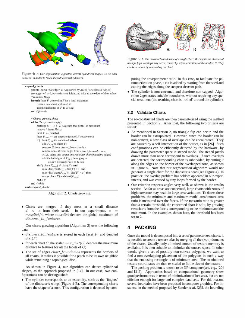
Figure 4: A: Our segmentation algorithm detects cylindrical shapes; B: An addi-

tional cut is added to ‘sock-shaped’ extremal cylinders.

expand_chartspriority_queue<halfedge>Heap sorted bydist(facet(halfedge))set<edge>chart_boundaries initialized with all the edges of the surface// Initialize Heapforeach facetF where dist(F ) is a local maximum

create a new chart with seedFadd the halfedges ofF toHeap

end // foreach

// Charts-growing phasewhile(Heap is not empty)

halfedgeh← e ∈ Heap such that dist(e) is maximumremoveh fromHeap

facetF ← facet(h)facetFopp← the opposite facet ofF relative tohif ( chart(Fopp) is undefined )then

addFopp to chart(F )removeE from chart_boundariesremove non-extremal edges fromchart_boundaries,// (i.e. edges that do not link two other chart boundary edges)add the halfedges ofFopp belonging to

chart_boundaries toHeapelsif ( chart(Fopp) 6= chart(F ) and

max_dist(chart(F )) - dist(F ) < ε andmax_dist(chart(Fopp)) - dist(F ) < ε ) thenmerge chart(F ) and chart(Fopp)

end // ifend // while

end // expand_charts

Algorithm 2: Charts growing.

• Charts are merged if they meet at a small distanced < ε from their seed. In our experiments,ε =maxdist/4, wheremaxdist denotes the global maximum ofdistance_to_features.

Our charts growing algorithm (Algorithm 2) uses the followingdata:• distance_to_feature is stored in each facetF , and denoteddist(F );

• for each chartC, the scalarmax_dist(C) denotes the maximumdistance to features for all the facets ofC;

• The set of edgeschart_boundaries represents the borders ofall charts. It makes it possible for a patch to be its own neighborwhile remaining a topological disc.

As shown in Figure4, our algorithm can detect cylindricalshapes, as the approach proposed in [14]. In our case, two con-figurations can be distinguished:• The cylinder corresponds to an extremity, such as the ‘fingers’

of the dinosaur’s wings (Figure4-B). The corresponding chartshave the shape of a sock. This configuration is detected by com-

Figure 5:A: The dinosaur’s head made of a single chart; B: Despite the absence of

triangle flips, overlaps may occur, caused by self-intersections of the border; C: They

can be removed by subdividing the chart.

puting the area/perimeter ratio. In this case, to facilitate the pa-rameterization phase, a cut is added by starting from the seed andcutting the edges along the steepest-descent path.

• The cylinder is non-extremal, and therefore non-capped. Algo-rithm 2 generates suitable boundaries, without requiring any spe-cial treatment (the resulting chart is ‘rolled’ around the cylinder).

3.3 Validate Charts

The so-constructed charts are then parameterized using the methodpresented in Section 2. After that, the following two criteria aretested:• As mentioned in Section 2, no triangle flip can occur, and the

border can be extrapolated. However, since the border can benon-convex, a new class of overlaps can be encountered. Theyare caused by a self-intersection of the border, as in [26]. Suchconfigurations can be efficiently detected by the hardware, bydrawing the parameter space in stencil mode. The stencil pixelsdrawn more than once correspond to overlaps. If such overlapsare detected, the corresponding chart is subdivided, by cutting italong the edges on the border of the overlapped zone, as shownin Figure 5. Note that our segmentation algorithm would notgenerate a single chart for the dinosaur’s head (see Figure4). Inpractice, the overlap problem has seldom appeared in our exper-iments, and was caused by tiny loops formed by the border.

• Our criterion respects angles very well, as shown in the resultssection. As far as areas are concerned, large charts with zones ofhigh curvature may result in large area variations. To detect theseproblems, the minimum and maximum model area/texture arearatio is measured over the facets. If the max/min ratio is greaterthan a certain threshold, the concerned chart is split, by growingtwo charts from the facets corresponding to the minimum and themaximum. In the examples shown here, the threshold has beenset to 2.

4 PACKING

Once the model is decomposed into a set of parameterized charts, itis possible to create a texture atlas by merging all the(u, v) domainsof the charts. Usually, only a limited amount of texture memory isavailable. It is then suitable to minimize the unused space. In otherwords, given a set of possibly non-convex polygons, we want tofind a non-overlapping placement of the polygons in such a waythat the enclosing rectangle is of minimum area. The so-obtainedtexture coordinates are then re-scaled to fit the size of the texture.

The packing problem is known to be NP-complete (see, e.g., [20]and [21]). Approaches based on computational geometry showgood performances in terms of minimization of lost area, but are notefficient enough for large and complex data sets. For this reason,several heuristics have been proposed in computer graphics. For in-stance, in the method proposed by Sanderet al. [25], the bounding

A B

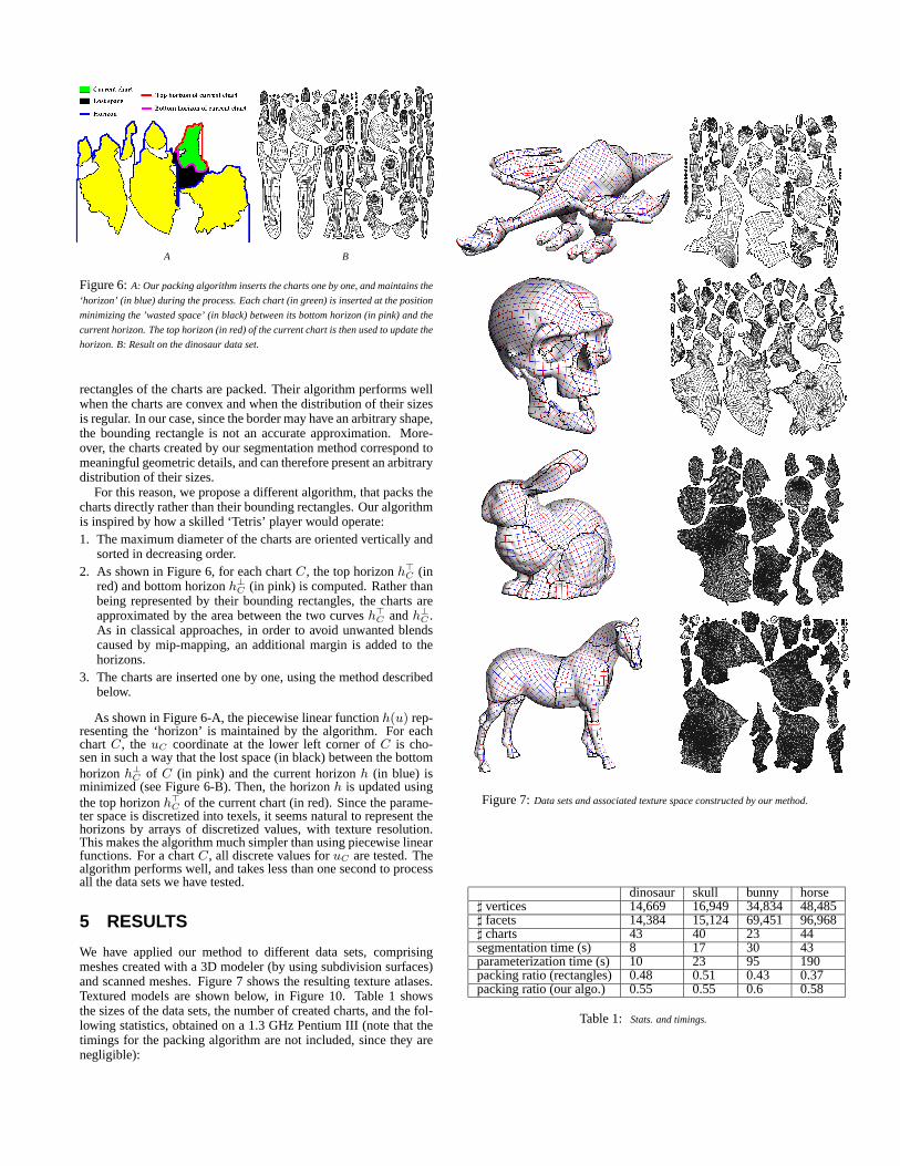
Figure 6:A: Our packing algorithm inserts the charts one by one, and maintains the

‘horizon’ (in blue) during the process. Each chart (in green) is inserted at the position

minimizing the ’wasted space’ (in black) between its bottom horizon (in pink) and the

current horizon. The top horizon (in red) of the current chart is then used to update the

horizon. B: Result on the dinosaur data set.

rectangles of the charts are packed. Their algorithm performs wellwhen the charts are convex and when the distribution of their sizesis regular. In our case, since the border may have an arbitrary shape,the bounding rectangle is not an accurate approximation. More-over, the charts created by our segmentation method correspond tomeaningful geometric details, and can therefore present an arbitrarydistribution of their sizes.

For this reason, we propose a different algorithm, that packs thecharts directly rather than their bounding rectangles. Our algorithmis inspired by how a skilled ‘Tetris’ player would operate:1. The maximum diameter of the charts are oriented vertically and

sorted in decreasing order.2. As shown in Figure6, for each chartC, the top horizonh>C (in

red) and bottom horizonh⊥C (in pink) is computed. Rather thanbeing represented by their bounding rectangles, the charts areapproximated by the area between the two curvesh>C andh⊥C .As in classical approaches, in order to avoid unwanted blendscaused by mip-mapping, an additional margin is added to thehorizons.

3. The charts are inserted one by one, using the method describedbelow.

As shown in Figure6-A, the piecewise linear functionh(u) rep-resenting the ‘horizon’ is maintained by the algorithm. For eachchartC, theuC coordinate at the lower left corner ofC is cho-sen in such a way that the lost space (in black) between the bottomhorizonh⊥C of C (in pink) and the current horizonh (in blue) isminimized (see Figure6-B). Then, the horizonh is updated usingthe top horizonh>C of the current chart (in red). Since the parame-ter space is discretized into texels, it seems natural to represent thehorizons by arrays of discretized values, with texture resolution.This makes the algorithm much simpler than using piecewise linearfunctions. For a chartC, all discrete values foruC are tested. Thealgorithm performs well, and takes less than one second to processall the data sets we have tested.

5 RESULTS

We have applied our method to different data sets, comprisingmeshes created with a 3D modeler (by using subdivision surfaces)and scanned meshes. Figure7 shows the resulting texture atlases.Textured models are shown below, in Figure10. Table1 showsthe sizes of the data sets, the number of created charts, and the fol-lowing statistics, obtained on a 1.3 GHz Pentium III (note that thetimings for the packing algorithm are not included, since they arenegligible):

Figure 7:Data sets and associated texture space constructed by our method.

dinosaur skull bunny horse] vertices 14,669 16,949 34,834 48,485] facets 14,384 15,124 69,451 96,968] charts 43 40 23 44segmentation time (s) 8 17 30 43parameterization time (s) 10 23 95 190packing ratio (rectangles) 0.48 0.51 0.43 0.37packing ratio (our algo.) 0.55 0.55 0.6 0.58

Table 1: Stats. and timings.

0

500

1000

1500

2000

2500

3000

80 85 90 95 100

angle deformations

0

100

200

300

400

500

600

0 0.5 1 1.5 2 2.5 3

area deformations

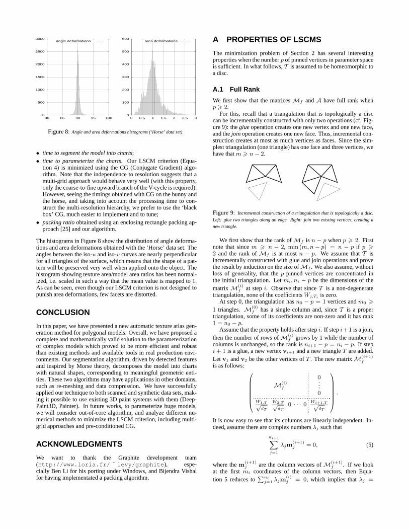
Figure 8:Angle and area deformations histograms (‘Horse’ data set).

• time to segment the model into charts;• time to parameterize the charts. Our LSCM criterion (Equa-

tion 4) is minimized using the CG (Conjugate Gradient) algo-rithm. Note that the independence to resolution suggests that amulti-grid approach would behave very well (with this property,only the coarse-to-fine upward branch of the V-cycle is required).However, seeing the timings obtained with CG on the bunny andthe horse, and taking into account the processing time to con-struct the multi-resolution hierarchy, we prefer to use the ‘blackbox’ CG, much easier to implement and to tune;

• packing ratioobtained using an enclosing rectangle packing ap-proach [25] and our algorithm.

The histograms in Figure8 show the distribution of angle deforma-tions and area deformations obtained with the ‘Horse’ data set. Theangles between the iso-u and iso-v curves are nearly perpendicularfor all triangles of the surface, which means that the shape of a pat-tern will be preserved very well when applied onto the object. Thehistogram showing texture area/model area ratios has been normal-ized, i.e. scaled in such a way that the mean value is mapped to 1.As can be seen, even though our LSCM criterion is not designed topunish area deformations, few facets are distorted.

CONCLUSION

In this paper, we have presented a new automatic texture atlas gen-eration method for polygonal models. Overall, we have proposed acomplete and mathematically valid solution to the parameterizationof complex models which proved to be more efficient and robustthan existing methods and available tools in real production envi-ronments. Our segmentation algorithm, driven by detected featuresand inspired by Morse theory, decomposes the model into chartswith natural shapes, corresponding to meaningful geometric enti-ties. These two algorithms may have applications in other domains,such as re-meshing and data compression. We have successfullyapplied our technique to both scanned and synthetic data sets, mak-ing it possible to use existing 3D paint systems with them (Deep-Paint3D, Painter). In future works, to parameterize huge models,we will consider out-of-core algorithm, and analyze different nu-merical methods to minimize the LSCM criterion, including multi-grid approaches and pre-conditioned CG.

ACKNOWLEDGMENTS

We want to thank the Graphite development team(http://www.loria.fr/ ˜ levy/graphite ), espe-cially Ben Li for his porting under Windows, and Bijendra Vishalfor having implementated a packing algorithm.

A PROPERTIES OF LSCMS

The minimization problem of Section2 has several interestingproperties when the numberp of pinned vertices in parameter spaceis sufficient. In what follows,T is assumed to be homeomorphic toa disc.

A.1 Full Rank

We first show that the matricesMf andA have full rank whenp > 2.

For this, recall that a triangulation that is topologically a disccan be incrementally constructed with only two operations (cf. Fig-ure9): theglueoperation creates one new vertex and one new face,and thejoin operation creates one new face. Thus, incremental con-struction creates at most as much vertices as faces. Since the sim-plest triangulation (one triangle) has one face and three vertices, wehave thatm > n− 2.

Figure 9: Incremental construction of a triangulation that is topologically a disc.

Left: glue two triangles along an edge. Right: join two existing vertices, creating a

new triangle.

We first show that the rank ofMf is n − p whenp > 2. Firstnote that sincem > n − 2, min (m,n− p) = n − p if p >2 and the rank ofMf is at mostn − p. We assume thatT isincrementally constructed with glue and join operations and provethe result by induction on the size ofMf . We also assume, withoutloss of generality, that thep pinned vertices are concentrated inthe initial triangulation. Letmi, ni − p be the dimensions of thematrixM(i)

f at stepi. Observe that sinceT is a non-degeneratetriangulation, none of the coefficientsWj,Ti is zero.

At step 0, the triangulation hasn0 − p = 1 vertices andm0 >1 triangles.M(0)

f has a single column and, sinceT is a propertriangulation, some of its coefficients are non-zero and it has rank1 = n0 − p.

Assume that the property holds after stepi. If stepi+1 is a join,then the number of rows ofM(i)

f grows by 1 while the number ofcolumns is unchanged, so the rank isni+1 − p = ni − p. If stepi + 1 is a glue, a new vertexvi+1 and a new triangleT are added.Let v1 andv2 be the other vertices ofT . The new matrixM(i+1)

fis as follows:

M(i)f

0...0

W1,T√dT

W2,T√dT

0 · · · 0Wi+1,T√

dT

.

It is now easy to see that its columns are linearly independent. In-deed, assume there are complex numbersλj such that

ni+1∑j=1

λjm(i+1)j = 0, (5)

where them(i+1)j are the column vectors ofM(i+1)

f . If we lookat the firstmi coordinates of the column vectors, then Equa-tion 5 reduces to

∑nij=1 λjm

(i)j = 0, which implies thatλj =

0, j = 1, . . . , ni, sinceM(i)f has full rank. Now the equa-

tion linking the last coordinate of the vectorsm(i+1)j reduces to

λni+1Wi+1,T /√dT = 0, implying thatλni+1 = 0. Thus the

columns ofM(i+1)f are linearly independent and the matrix has

full rank. The result is proved.SinceMf has rankn − p, bothM1

f andM2f have rankn − p

whenp > 2. In turn, this implies thatA has rank2(n − p) whenp > 2.

A.2 Single Minimum

We now show that, whenp > 2, C(U) has a unique minimum.First, notice that

∂C

∂x= 2(A>Ax−A>b).

Now, since the rank of the Gram matrix ofA (i.e. A>A) is thesame as the rank ofA,A>A has rank2(n− p) whenp > 2. SinceA>A is a square2(n − p) × 2(n − p) matrix, it is thus invertibleand the minimization problem has a unique solution (whenp > 2)

x = (A>A)−1A>b.

The minimum ofC(U) is zero whenAx = b, i.e. whenA isinvertible. Since it has full rank, this happens exactly whenA issquare, i.e. whenm = n − p. Using the fact thatm > n − 2,this implies thatp = 2. We conclude that the mappingU is fullyconformal (barring self-intersections) exactly whenp = 2 and thetriangulationT is built only with glue operations.

A.3 Invariance by Similarity

We now prove that ifU is a solution to the minimization prob-lem, thenzU + T is also a solution, for allz ∈ C and T =(z′, . . . , z′), z′ ∈ C. In other words, the problem is invariant bya similarity transformation.

First note that the vectorH = (1, . . . , 1)> is trivially in thekernel ofM, sinceW1 +W2 +W3 = 0 in each triangle. AssumeU is a solution of the problem. We get:

C(zU + T) = zz C(U) + 2zT∗CU,= zz C(U) + 2z(MT)∗MU = zz C(U),

becauseT = z′H is in the kernel ofM. If C(U) = 0, thenC(zU + T) = 0.

A.4 Independence to Resolution

We now show that if a given mesh is ‘densified’, then the solution tothe augmented optimization problem restricted to the vertices of theinitial mesh is the same. We prove this result when a single triangleT is split into three triangles, but the proof generalizes easily toa more general setting. So letv be the new vertex introduced intriangleT , i.e. as a linear combination of verticesv1,v2,v3:

v =

3∑i=1

αivi,

3∑i=1

αi = 1, αi > 0.

Assume also for the sake of simplicity that none ofv,v1,v2,v3

is pinned. CallTi (i = 1, . . . , 3) the triangle created that does nothavevi as vertex. Then it is easy to see thatdTi = αidT .Mf is anm × (n − p) matrix. After insertion ofv, the new

matrixM+f is (m+ 2)× (n+ 1− p). Indeed, one vertex is added,

augmenting the number of columns by one, and three new triangles

replace an old one, augmenting the number of rows by two. Thestructure of these matrices is as follows:

Mf =

Nf

F 0 · · · 0

, M+f =

Nf

0...0

L 0 P

.

whereNf is an(m−1)×(n−p) matrix,F is 1×3,L is 3×3 andPis 3× 1. If the coefficients ofF are denoted byfj = Wj,T /

√dT ,

then it is easy to observe that the coefficients ofL = (lij) andP = (pi) satisfy

lij =1√αi

(αifj − αjfi

), pi =

1√αifi. (6)

The(n− p)× 1 solution to the initial problem is:

Uf = (M∗fMf )(−1)M∗fMpUp.

Consider the(n+ 1− p)× 1 solution to the augmented problem:

U+f = (M+

f

∗M+f )(−1)M+

f

∗M+p U+

p . (7)

Using the relations of Equation6 and the fact thatf1 +f2 +f3 = 0,it suffices then to observe thatU+

f = (U>f , Uv)> is the (unique)solution to7, where

Uv = α1U1 + α2U2 + α3U3.

In other words, the least squares conformal parameterization is un-changed at the old vertices and is the barycenter of the parameteri-zations ofv1,v2 andv3 at the new vertexv.

A.5 Preserving Orientations

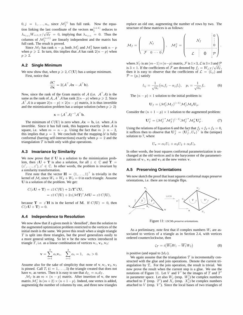
We now sketch the proof that least squares conformal maps preserveorientations, i.e. there are no triangle flips.

2U

3U

V 2

V 1V 3

V

T T’ V UV’

U 1u

v

LSCM

Figure 11:LSCMs preserve orientations.

As a preliminary, note first that if complex numbersWi are as-sociated to vertices of a triangle as in Section2.4, with verticesordered counterclockwise, then

ζT = i(W2W1 −W1W2

)(8)

is positive (and equal to2dT ).We again assume that the triangulationT is incrementally con-

structed with the glue and join operations. Denote the current tri-angulation byTi. For the join operation, the result is trivial. Wenow prove the result when the current step is a glue. We use thenotations of Figure11. Let V andV ′ be the images ofT andT ′

in parameter space. Let alsoWj (resp.W ′j ) be complex numbersattached toT (resp. T ′) andXj (resp.X ′j) be complex numbersattached toV (resp.V ′). Since the local bases of two triangles of

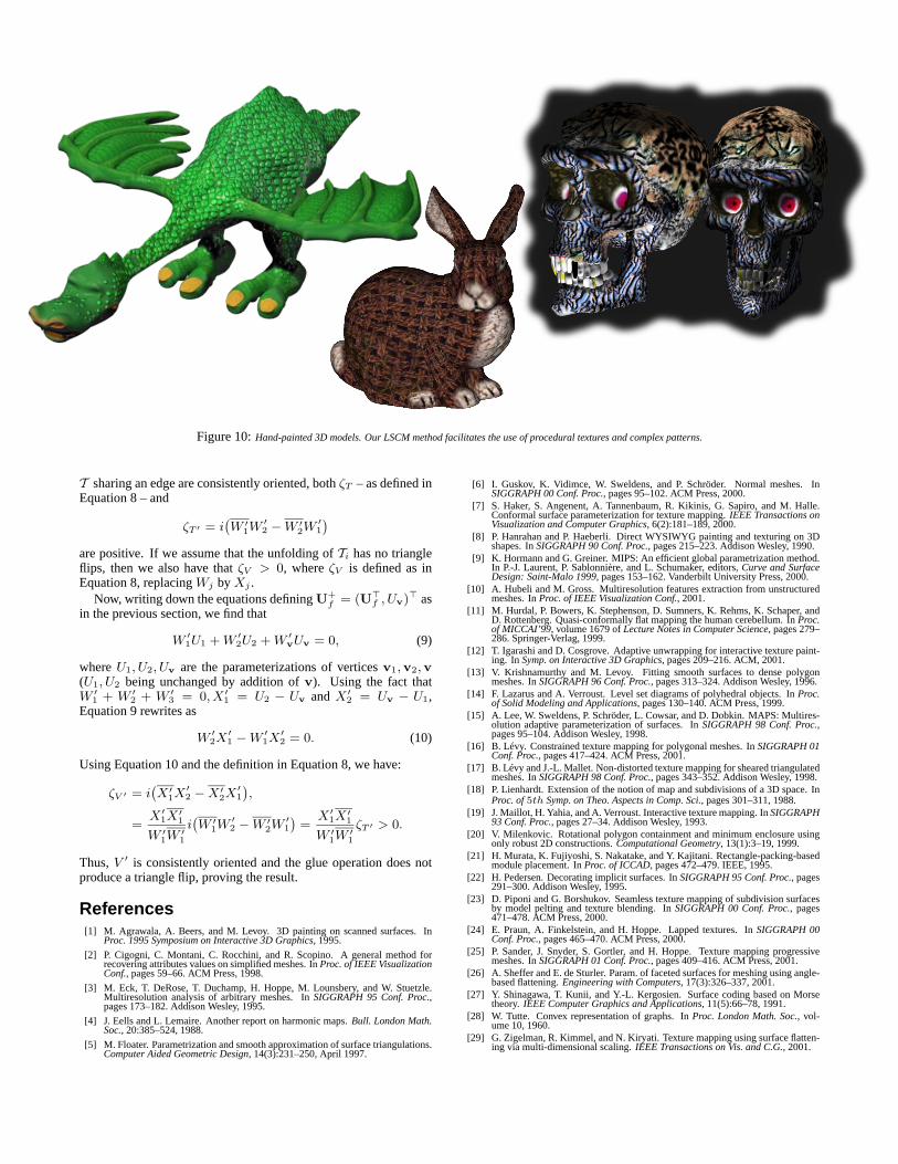
Figure 10:Hand-painted 3D models. Our LSCM method facilitates the use of procedural textures and complex patterns.

T sharing an edge are consistently oriented, bothζT – as defined inEquation8 – and

ζT ′ = i(W ′1W

′2 −W ′2W

′1

)are positive. If we assume that the unfolding ofTi has no triangleflips, then we also have thatζV > 0, whereζV is defined as inEquation8, replacingWj byXj .

Now, writing down the equations definingU+f = (U>f , Uv)> as

in the previous section, we find that

W ′1U1 +W ′2U2 +W ′vUv = 0, (9)

whereU1, U2, Uv are the parameterizations of verticesv1,v2,v(U1, U2 being unchanged by addition ofv). Using the fact thatW ′1 + W ′2 + W ′3 = 0, X ′1 = U2 − Uv andX ′2 = Uv − U1,Equation9 rewrites as

W ′2X′1 −W ′1X ′2 = 0. (10)

Using Equation10and the definition in Equation8, we have:

ζV ′ = i(X ′1X

′2 −X ′2X

′1

),

=X ′1X

′1

W ′1W′1

i(W ′1W

′2 −W ′2W

′1

)=X ′1X

′1

W ′1W′1

ζT ′ > 0.

Thus,V ′ is consistently oriented and the glue operation does notproduce a triangle flip, proving the result.

References[1] M. Agrawala, A. Beers, and M. Levoy. 3D painting on scanned surfaces. In

Proc. 1995 Symposium on Interactive 3D Graphics, 1995.

[2] P. Cigogni, C. Montani, C. Rocchini, and R. Scopino. A general method forrecovering attributes values on simplified meshes. InProc. of IEEE VisualizationConf., pages 59–66. ACM Press, 1998.

[3] M. Eck, T. DeRose, T. Duchamp, H. Hoppe, M. Lounsbery, and W. Stuetzle.Multiresolution analysis of arbitrary meshes. InSIGGRAPH 95 Conf. Proc.,pages 173–182. Addison Wesley, 1995.

[4] J. Eells and L. Lemaire. Another report on harmonic maps.Bull. London Math.Soc., 20:385–524, 1988.

[5] M. Floater. Parametrization and smooth approximation of surface triangulations.Computer Aided Geometric Design, 14(3):231–250, April 1997.

[6] I. Guskov, K. Vidimce, W. Sweldens, and P. Schröder. Normal meshes. InSIGGRAPH 00 Conf. Proc., pages 95–102. ACM Press, 2000.

[7] S. Haker, S. Angenent, A. Tannenbaum, R. Kikinis, G. Sapiro, and M. Halle.Conformal surface parameterization for texture mapping.IEEE Transactions onVisualization and Computer Graphics, 6(2):181–189, 2000.

[8] P. Hanrahan and P. Haeberli. Direct WYSIWYG painting and texturing on 3Dshapes. InSIGGRAPH 90 Conf. Proc., pages 215–223. Addison Wesley, 1990.

[9] K. Hormann and G. Greiner. MIPS: An efficient global parametrization method.In P.-J. Laurent, P. Sablonnière, and L. Schumaker, editors,Curve and SurfaceDesign: Saint-Malo 1999, pages 153–162. Vanderbilt University Press, 2000.

[10] A. Hubeli and M. Gross. Multiresolution features extraction from unstructuredmeshes. InProc. of IEEE Visualization Conf., 2001.

[11] M. Hurdal, P. Bowers, K. Stephenson, D. Sumners, K. Rehms, K. Schaper, andD. Rottenberg. Quasi-conformally flat mapping the human cerebellum. InProc.of MICCAI’99, volume 1679 ofLecture Notes in Computer Science, pages 279–286. Springer-Verlag, 1999.

[12] T. Igarashi and D. Cosgrove. Adaptive unwrapping for interactive texture paint-ing. In Symp. on Interactive 3D Graphics, pages 209–216. ACM, 2001.

[13] V. Krishnamurthy and M. Levoy. Fitting smooth surfaces to dense polygonmeshes. InSIGGRAPH 96 Conf. Proc., pages 313–324. Addison Wesley, 1996.

[14] F. Lazarus and A. Verroust. Level set diagrams of polyhedral objects. InProc.of Solid Modeling and Applications, pages 130–140. ACM Press, 1999.

[15] A. Lee, W. Sweldens, P. Schröder, L. Cowsar, and D. Dobkin. MAPS: Multires-olution adaptive parameterization of surfaces. InSIGGRAPH 98 Conf. Proc.,pages 95–104. Addison Wesley, 1998.

[16] B. Lévy. Constrained texture mapping for polygonal meshes. InSIGGRAPH 01Conf. Proc., pages 417–424. ACM Press, 2001.

[17] B. Lévy and J.-L. Mallet. Non-distorted texture mapping for sheared triangulatedmeshes. InSIGGRAPH 98 Conf. Proc., pages 343–352. Addison Wesley, 1998.

[18] P. Lienhardt. Extension of the notion of map and subdivisions of a 3D space. InProc. of5th Symp. on Theo. Aspects in Comp. Sci., pages 301–311, 1988.

[19] J. Maillot, H. Yahia, and A. Verroust. Interactive texture mapping. InSIGGRAPH93 Conf. Proc., pages 27–34. Addison Wesley, 1993.

[20] V. Milenkovic. Rotational polygon containment and minimum enclosure usingonly robust 2D constructions.Computational Geometry, 13(1):3–19, 1999.

[21] H. Murata, K. Fujiyoshi, S. Nakatake, and Y. Kajitani. Rectangle-packing-basedmodule placement. InProc. of ICCAD, pages 472–479. IEEE, 1995.

[22] H. Pedersen. Decorating implicit surfaces. InSIGGRAPH 95 Conf. Proc., pages291–300. Addison Wesley, 1995.

[23] D. Piponi and G. Borshukov. Seamless texture mapping of subdivision surfacesby model pelting and texture blending. InSIGGRAPH 00 Conf. Proc., pages471–478. ACM Press, 2000.

[24] E. Praun, A. Finkelstein, and H. Hoppe. Lapped textures. InSIGGRAPH 00Conf. Proc., pages 465–470. ACM Press, 2000.

[25] P. Sander, J. Snyder, S. Gortler, and H. Hoppe. Texture mapping progressivemeshes. InSIGGRAPH 01 Conf. Proc., pages 409–416. ACM Press, 2001.

[26] A. Sheffer and E. de Sturler. Param. of faceted surfaces for meshing using angle-based flattening.Engineering with Computers, 17(3):326–337, 2001.

[27] Y. Shinagawa, T. Kunii, and Y.-L. Kergosien. Surface coding based on Morsetheory. IEEE Computer Graphics and Applications, 11(5):66–78, 1991.

[28] W. Tutte. Convex representation of graphs. InProc. London Math. Soc., vol-ume 10, 1960.

[29] G. Zigelman, R. Kimmel, and N. Kiryati. Texture mapping using surface flatten-ing via multi-dimensional scaling.IEEE Transactions on Vis. and C.G., 2001.