Embed Size (px)
Citation preview

Lec 10: Introduc/on to BTE and
Monte Carlo Method

Let’s play a game
0
1
2
3
4
5
6
7
8
9
... Let’s build a high‐rise building
• each storey has one room • 6 persons, 9 /ckets • if you get one /cket, you move up one level • How many ways there are to distribute 9 /ckets to 6 people?
Example taken from BlaR, Frank J.,Modern Physics, McGraw‐Hill, (1992), Sec/on 11.4

9 Tickets, 6 People
• plan 1:
ways in this plan
0
1
2
3
4
5
6
7
8
9
...
€
6!5!×1!
= 6

9 Tickets, 6 People
0
1
2
3
4
5
6
7
8
9
... • plan 2:
ways
€
6!3!×2!×1!
= 60

9 Tickets, 6 People
0
1
2
3
4
5
6
7
8
9
... • plan 3:
ways
€
6!2!×2!×1!×1!
=180

26 plans, 2002 ways

Let’s count the numbers
Storey Average number
0 2.143
1 1.484
2 0.989
3 0.629
4 0.378
5 0.210
6 0.105
7 0.045
8 0.015
9 0.003

Let’s make the game more fun
• each storey has different number of rooms
• each person can freely choose in which room (on the storey) he likes to enter
• previous count:
• new count: 20×23 = 160 0
1
2
3
4
5
6
7
8
9
...
€
6!3!×3!
= 20
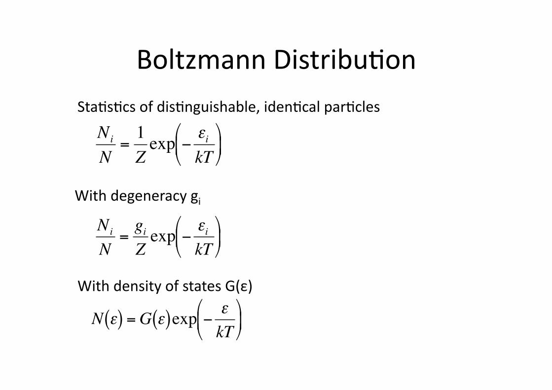
Boltzmann Distribu/on
€
Ni
N=1Zexp − εi
kT
€
Ni
N=giZexp − εi
kT
With degeneracy gi
€
N ε( ) =G ε( )exp − εkT
With density of states G(ε)
Sta/s/cs of dis/nguishable, iden/cal par/cles

DOS of Ideal Gas
dv v vx
vy
vz states between velocity v and v+dv
€
∝dv ⋅v 2
states between energy ε and ε+dε
€
∝dε ⋅ ε dvdε
= dε ε
kine/c energy
€
ε =12mv 2
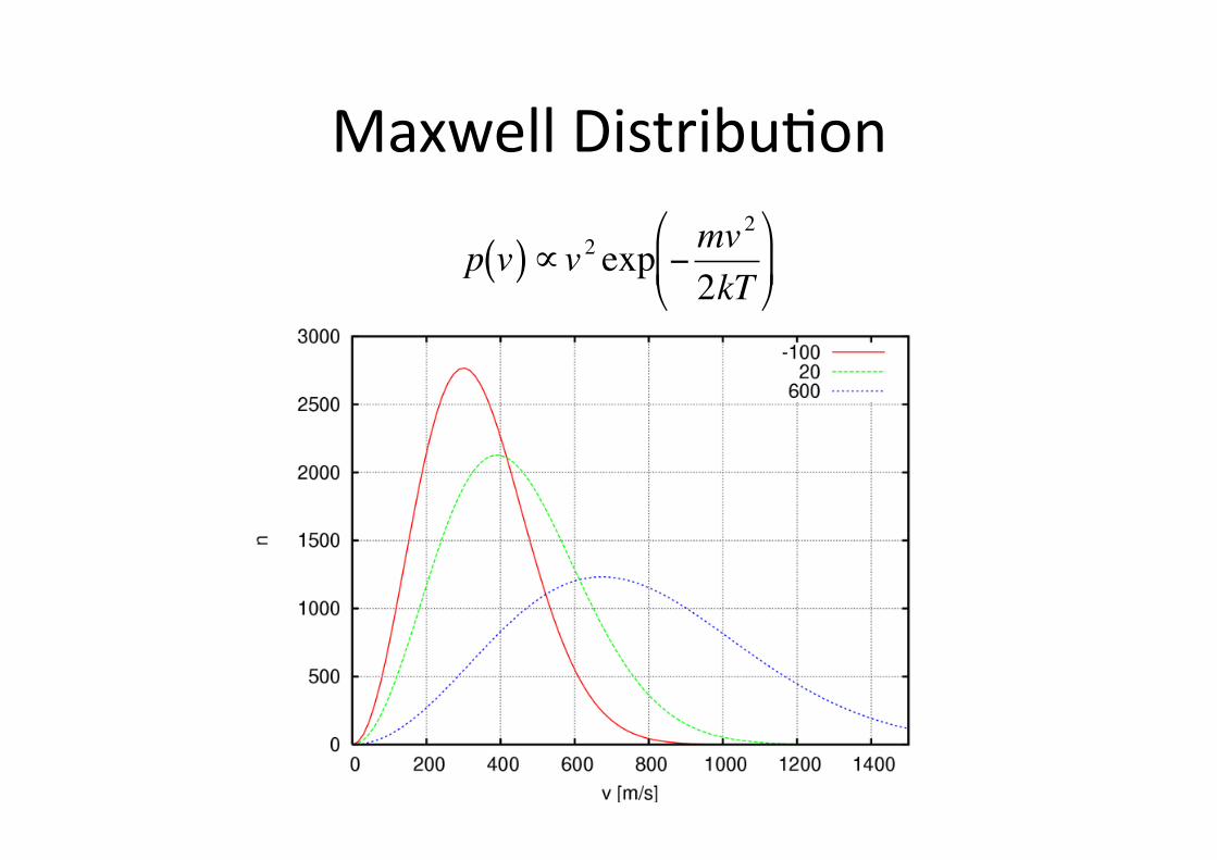
Maxwell Distribu/on
€
p v( )∝v 2 exp −mv2
2kT

In semiconductors
• Fermi distribu/on v.s. Boltzmann distribu/on • we have a band‐gap with zero DOS
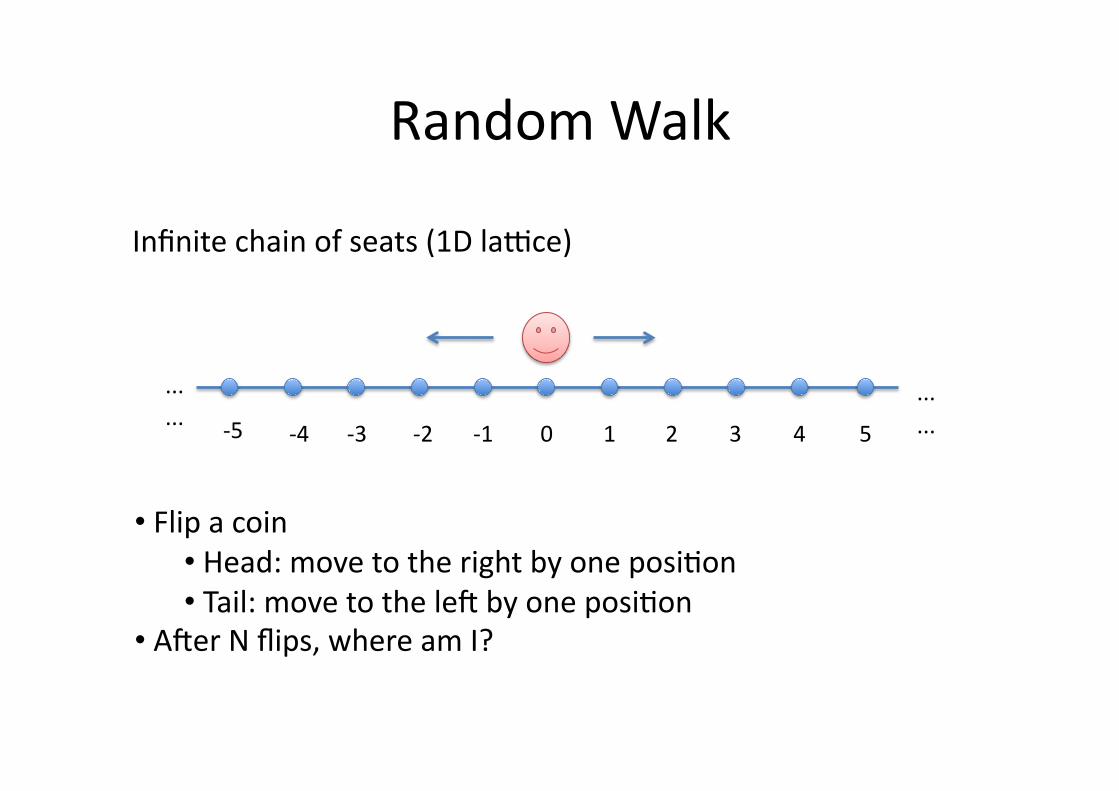
Random Walk
Infinite chain of seats (1D laece)
... ...
• Flip a coin • Head: move to the right by one posi/on • Tail: move to the lef by one posi/on
• Afer N flips, where am I?
0 1 2 3 4 5 ‐1 ‐2 ‐3 ‐4 ‐5 ... ...

Random Walk
... ...
0 1 2 3 4 5 ‐1 ‐2 ‐3 ‐4 ‐5 ... ...
Afer 4 flips, what’s the probability of being at posi/on 0?
Out of 24 = 16 possible out comes from the tosses,
we must have 2 Heads and 2 Tails, that is .
So the probability is 6/16.
€
4!2!×2!
= 6

Random Walk
... ...
0 1 2 3 4 5 ‐1 ‐2 ‐3 ‐4 ‐5 ... ...
Afer 4 flips, what’s the probability of being at posi/on n ?
€
4!2!×2!
= 6
‐4 ‐3 ‐2 ‐1 0 1 2 3 4
1/16 0 4/16 0 6/16 0 4/16 0 1/16
€
4!3!×1!
= 4
€
4!4!×0!
=1
€
4!1!×3!
= 4
€
4!0!×4!
=1

Random Walk
N ‐5 ‐4 ‐3 ‐2 ‐1 0 1 2 3 4 5
0 1
1 1 1
2 1 2 1
3 1 3 3 1
4 1 4 6 4 1
5 1 5 10 10 5 1
...
Afer N flips, the probability of being at posi/on n

For Large Number of N
! "
#$%&!'%((!$)**+,!%-!.$+!,/01+2!3-!-32')24!&.+*&!+56++4&!.$+!,/01+2!3-!1)67')24!&.+*&!18!n!
9'$%6$!63/(4!1+!)!,+:).%;+!,/01+2<=!!
!
#$).!%&>!
-32')24 1)67')24
-32')24 1)67')24 ?@@
n n n
n n
! "
# "!
-230!'$%6$!!
$ % $ %? ?-32')24 1)67')24A A
?@@ > ?@@ =n n n" # " ! n !
!
B3.+!.$).!%,!.$+!:+,+2)(!6)&+>!%-!.$+!.3.)(!,/01+2!3-!&.+*&!N!%&!+;+,>! !)2+!13.$!+;+,!
32!13.$!344>!&3!n>!.$+!4%--+2+,6+!1+.'++,!.$+0>!%&!+;+,>!),4!&%0%()2(8!344!N!0+),&!344!n=!!
-32')24 1)67')24>n n
!
#$+!.3.)(!,/01+2!3-!*).$&!+,4%,:!).!.$+!*)2.%6/()2!*3%,.!n>!-230!.$+!$+)4&!),4!.)%(&!)2:/0+,.!
)13;+>!%&!
$ % $ % $ %$ % $ %$ %? ?-32')24 1)67')24 A A
?@@C ?@@C=
C C ?@@ C ?@@ Cn n n n"
# !!
!
#3!-%,4!.$+!)6./)(!*231)1%(%.8!3-!+,4%,:!).!,!)-.+2!?@@!&.+*&>!'+!,++4!.3!7,3'!'$).!-2)6.%3,!3-!)((!
*3&&%1(+!*).$&!+,4!).!n=!9D%,6+!.$+!63%,!.3&&!%&!*/2+(8!2),430>!'+!.)7+!%.!)((!*3&&%1(+!*).$&!)2+!
+E/)((8!(%7+(8<=!!#$+!total!,/01+2!3-!*3&&%1(+!?@@F&.+*!')(7&!%&! !?@@ G@A ?=AH ?@& ' =
!
I+J;+!/&+4!K56+(!.3!*(3.!.$+!2).%3L!9,/01+2!3-!*).$&!+,4%,:!).!n<M9.3.)(!,/01+2!3-!*).$&<!!
-32!*).$&!3-!?@@!2),430!&.+*&>!),4!-%,4L!
!
0
0.01
0.02
0.03
0.04
0.05
0.06
0.07
0.08
0.09
-48 -40 -32 -24 -16 -8 0 8 16 24 32 40 48
final position n after 100 steps
pro
bab
ilit
y o
f la
nd
ing
at n
!!
€
P n( ) =22πN
exp − n2
2N
Afer N flips, the probability of being at posi/on n:

Random Walk and Diffusion • Uniformly distributed green molecules in the background • A (thin) tube of red molecules released at x=0 • How are the red molecules distributed afer /me t
x 0
A simplest model: ‐ Molecules move independent of each other ‐ At each moment, each molecule has equal chance to move to lef/right, by a unit length ‐ This is random walk.
A beRer model is the Weiner process

Random Walk and Diffusion
€
P n( ) =22πN
exp − n2
2N
€
G x, t( ) =14πDt
exp − x 2
4Dt
Random Walk:
€
∂u∂t
= D∂2u∂x 2
u x, t = 0( ) = δ x( )
Diffusion star/ng from a delta func/on distribu/on
(Green’s func/on)
Diffusion is the macroscopic manifest of random mo/on of par/cles.

Microscopic v.s. Macroscopic Picture
• Microscopic Picture – probability of micro‐states
– transi/on between micro‐states
• Macroscopic Picture – distribu/on func/ons – differen/al equa/on to describe the evolu/on of the distribu/on func/on

Distribu/on func/on in device
€
f x,y,z, px, pz, pz,t( )
In equilibrium
p
€
f = exp − εkT
= exp −
v 2
2mkT
6+1 dimensions

Boltzmann Transport Equa/on
€
∂f∂t
= −v ⋅ ∇ r f + eF ⋅ ∇p f +∂f∂t
C
Collision accelera/on in external field
convec/on+ “diffusion”

Equilibrium
p
x
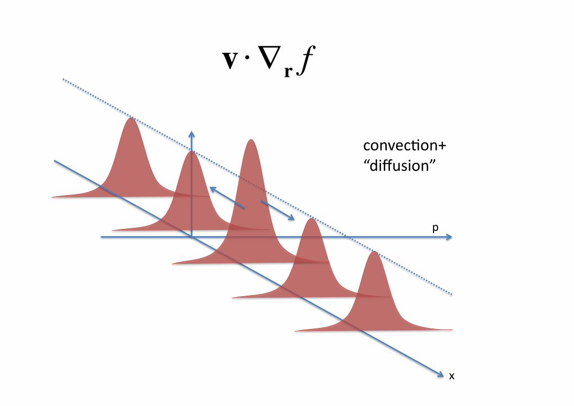
€
v ⋅ ∇ r f
p
x
convec/on+ “diffusion”

€
eF ⋅ ∇p f
p
Accelera/on in external field, deviate away from equilibrium

€
∂f∂t
C
p
ScaRering, returning to equilibrium
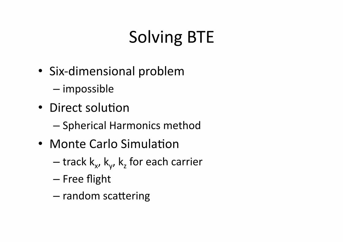
Solving BTE
• Six‐dimensional problem – impossible
• Direct solu/on – Spherical Harmonics method
• Monte Carlo Simula/on – track kx, ky, kz for each carrier – Free flight – random scaRering

Three Components of MC
• Free flight under external field F:
• Time of free flight: τ (Poisson distribu/on):
• ScaRering Rate: Γ
€
Δk = −eFhτ
€
P τ( ) = Γexp −Γτ( )

MC Flowchart
τ = free flight /me
start
free flight, update k
scaRer to new k
scaRered?

ScaRering
• Phonon ScaRering Mechanisms
218 5. Electrical Transport
+!
Ze
b
e-
K
Fig. 5.5. Coulomb scattering of anelectron by a positively charged ion.The impact parameter b and thelength K are discussed in the text.[Ref. 5.2, Fig. 4.1]
Conwell–Weisskopf Approach. In this approach an electron is assumed to bescattered classically via Coulomb interaction by an impurity ion with charge!Ze. The corresponding scattering cross section is calculated in exactly thesame way as for the Rutherford scattering of · particles [5.16]. The scatteringgeometry of this problem is shown schematically in Fig. 5.5. The scatteringcross section Û as a function of the scattering angle £ is given by
Û(£)dø " 2!b d |b | (5.53)
where dø is an element of solid angle, b is known as the impact parameter.and d |b | is the change in |b | required to cover the solid angle dø. The im-pact parameter and the solid angle dø are related to the scattering angle by
b " K cot(£/2); dø " 2! sin£d£ (5.54)
where K is a characteristic distance defined by
K "Ze2
mv2k
(5.55)
and vk is the velocity of an electron with energy Ek " mv2k/2. If dø and d |b |
are expressed in terms of d£, (5.53) can be simplified to
Û(£) "
!
K2 sin2(£/2)
"2
. (5.56)
The well-known dependence of Û on the electron velocity to the power of #4in Rutherford scattering is contained in the term K2. The scattering rate R(per unit time) of particles traveling with velocity v by N scattering centersper unit volume, each with scattering cross section Û, is given by
R " NÛv. (5.57)
Since scattering by impurities relaxes the momenta of carriers, but not their energy,we can define a momentum relaxation time Ùi due to impurity scattering by
1/Ùi " Nivk
#
Û(£)(1 # cos£)2! sin£d£, (5.58)
where Ni is the concentration of ionized impurities. Within the integrand, theterm (1 # cos£) is the fractional change in the electron momentum due toscattering event and the term 2! sin£d£ represents integration of the solid
Phonon ScaRering (deforma/on poten/al)
Coulomb scaRering
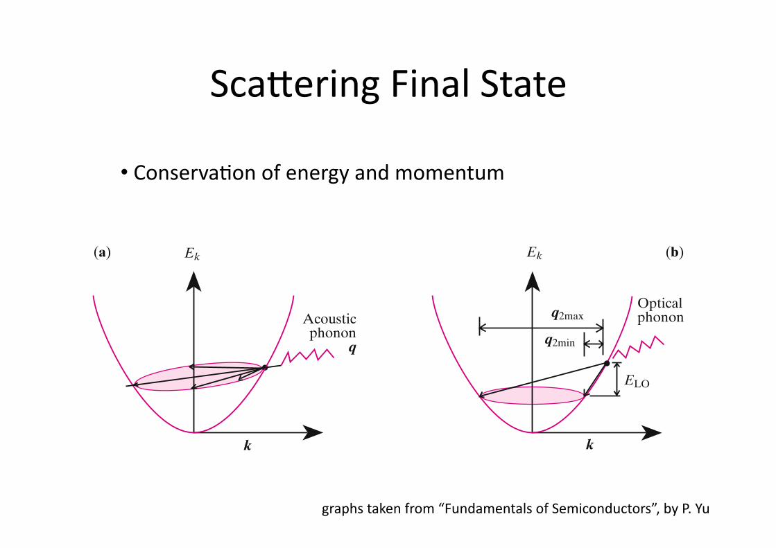
ScaRering Final State
210 5. Electrical Transport
For an acoustic phonon with a small q, Ep is related to q by
Ep ! "vsq, (5.36)
where vs is the phonon velocity. For simplicity we shall assume vs to beisotropic.
We shall further assume that the electron is in a parabolic band with ef-fective mass m! and it is scattered by acoustic phonons within the same band(this is known as intraband scattering). Since the scattering process conservesenergy and wave vector, the allowed values of q are obtained by combining(5.35) and (5.36) into
("2/2m!) (k2 # |k # q |2) ! "vsq (5.37)
and solving for q. The final electronic states, after emission of an acousticphonon, are shown schematically in Fig. 5.1a. From this picture it is clear thatthe allowed values of q lie between a minimum (qmin) and a maximum (qmax).For k $ mvs/", qmin is zero while qmax is reached when k" is diagonally oppo-site to k, i. e., when the electron is scattered by 180# (backscattering). From(5.37) qmax can easily be calculated to be
qmax ! 2k # (2mvs/"). (5.38)
The energy lost by the electron in emitting this phonon is
Ek # Ek" ! "vsqmax ! 2"vsk # 2mv2s . (5.39)
To estimate the order of magnitude of these quantities, we will assumethe following values of the parameters involved: m! ! 0.1m0 (m0 is the freeelectron mass), vs ! 106 cm/s, and Ek ! 25 meV (roughly corresponding toroom temperature times kB). For this electron k ! 2.6 $ 106 cm#1, qmax !5 $ 106 cm#1 % 2k, k" ! 2.4 $ 106 cm#1 (k" % #k) and Ek # Ek" ! 3.3 meV.In emitting an acoustic phonon with wave vector qmax, the electron completely
Ek
k
Ek
k
Acousticphonon
q
q2max
q2min
ELO
Opticalphonon
(b)(a)
Fig. 5.1. Schematic diagrams for the scattering of an electron in a parabolic band by emis-sion of (a) an acoustic phonon and (b) a longitudinal optical (LO) phonon showing thefinal electronic states and also the range of phonon wave vectors allowed by wave vectorconservation
graphs taken from “Fundamentals of Semiconductors”, by P. Yu
• Conserva/on of energy and momentum

ScaRering Rate
• Energy dependent • (maybe) angle dependent

Carrier Velocity and Mobility
226 5. Electrical Transport
ization time. Processes contributing to thermalization are carrier–carrier andcarrier–phonon interactions. As shown in Fig. 5.3, carrier–phonon interactiontimes can range from 0.1 ps (for polar optical phonons and for phonons inintervalley scattering) to tens of picoseconds (for acoustic phonons). Carrier–carrier interaction times depend strongly on carrier density. This has beenmeasured optically in GaAs. At high densities (!1018 cm"3) carriers thermal-ize in times as short as femtoseconds (equal to 10"15 s and abbreviated as fs)[5.25]. Thus the thermalization time is determined by carrier–carrier interac-tion at high carrier densities. At low densities, it is of the order of the shortestcarrier–phonon interaction time. Often carriers have a finite lifetime becausethey can be trapped by defects. If both electrons and holes are present, thecarrier lifetime is limited by recombination (Chap. 7). In samples with a veryhigh density of defects (such as amorphous semiconductors) carrier lifetimescan be picoseconds or less. Since the carrier lifetime determines the amountof time carriers have to thermalize, a distribution is a nonequilibrium onewhen the carrier lifetime is shorter than the thermalization time. A transientnonequilibrium situation can also be created by perturbing a carrier distribu-tion with a disturbance which lasts for less than the thermalization time.
The properties of hot carriers can be different from those of equilibriumcarriers. One example of this difference is the dependence of the drift velocityon electric field. Figure 5.12 shows the drift velocity in Si and GaAs as a func-tion of electric field. At fields below 103 V/cm, the carriers obey Ohm’s law,namely, the drift velocity increases linearly with the electric field. At higherfields the carrier velocity increases sublinearly with field and saturates at a ve-locity of about 107 cm/s. This leveling off of the carrier drift velocity at highfield is known as velocity saturation. n-Type GaAs shows a more complicatedbehavior in that its velocity has a maximum above the saturation velocity. Thisphenomenon is known as velocity overshoot (Fig. 5.12) and is found usuallyonly in a few n-type semiconductors such as GaAs, InP, and InGaAs. For
10
10
10
10
8
7
6
5
(Electrons)Si
GaAs (Electrons)
Si (Holes)
GaAs (Holes)
T=300K
10 10 10 10 102 3 4 5 6
Electric field [V/cm]
Dri
ft v
eloc
ity [c
m/s
]
Fig. 5.12. Dependence of drift velocity on electric field for electrons and holes in Si andGaAs [5.17]. Notice the velocity overshoot for electrons in GaAs

From BTE to Balance Equa/ons
€
∂f∂t
= −v ⋅ ∇ r f + eF ⋅ ∇p f +∂f∂t
C
BTE is Difficult to Solve We want to have a simpler equa/on ‐ Six‐dimension is too much ‐ try to eliminate the momentum dimensions ‐ yet the new equa/on should be physical
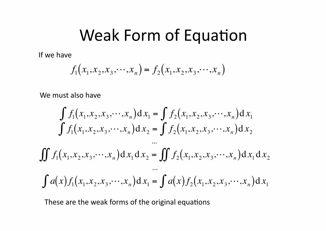
Weak Form of Equa/on
€
f1 x1,x2,x3,,xn( ) = f2 x1,x2,x3,,xn( )
€
f1 x1,x2,x3,,xn( )∫ d x1 = f2 x1,x2,x3,,xn( )d x1∫
If we have
We must also have
€
f1 x1,x2,x3,,xn( )d x1 d x2∫∫ = f2 x1,x2,x3,,xn( )d x1 d x2∫∫...
€
f1 x1,x2,x3,,xn( )∫ d x2 = f2 x1,x2,x3,,xn( )d x2∫...
€
a x( ) f1 x1,x2,x3,,xn( )∫ d x1 = a x( ) f2 x1,x2,x3,,xn( )d x1∫These are the weak forms of the original equa/ons

Moments of Distribu/on Func/on
€
f dp∫ = nZero‐th Moment Carrier Density
€
pf dp∫ = n p = npdFirst Moment Carrier Density x Average Momentum = Momentum Density
€
wf dp∫ = n wSecond Moment Carrier Density x Average Energy = Energy Density
€
f x,y,z, px, py, pz( )dp∫ = n x,y,z( )
by integra/ng over p, we eliminated the func/onal dependence on p
...
There could be higher moments, but they no longer have clear physical meaning

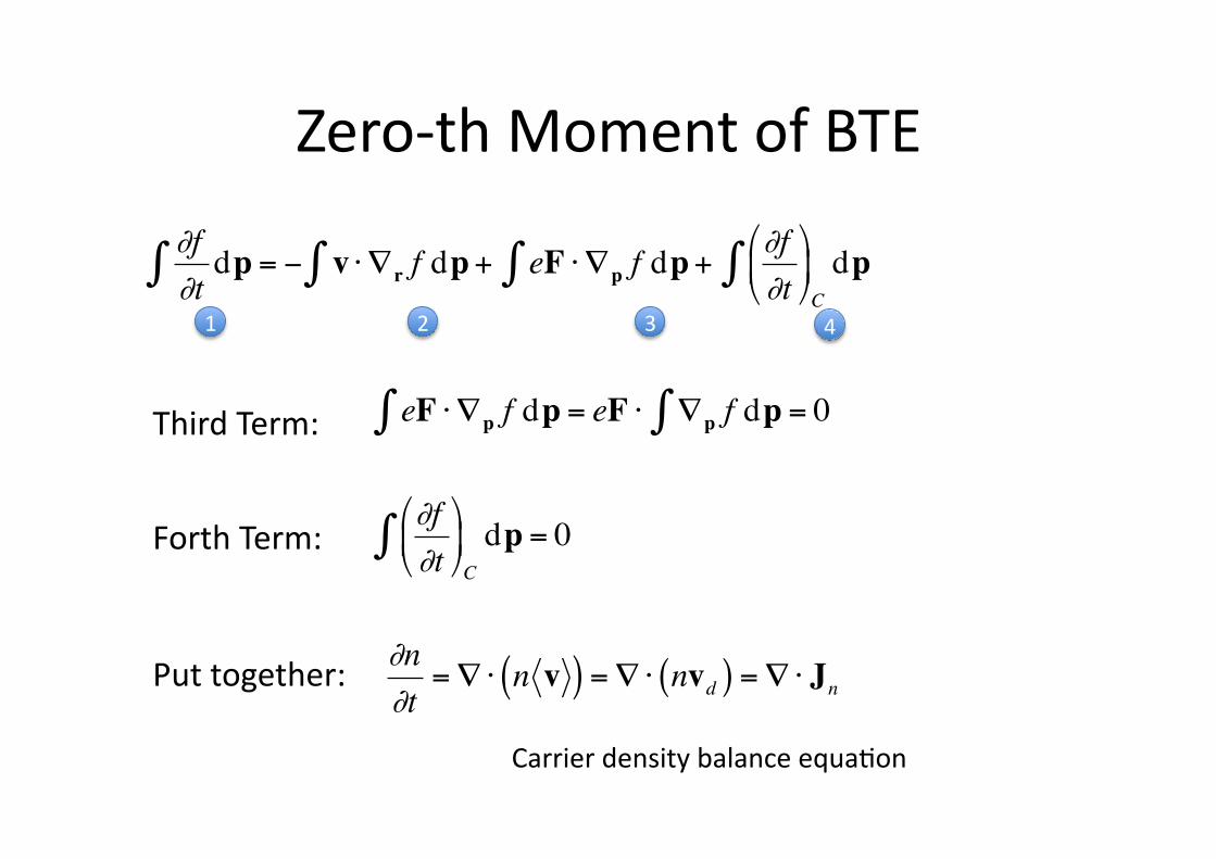
Zero‐th Moment of BTE
€
∂f∂t
= −v ⋅ ∇ r f + eF ⋅ ∇p f +∂f∂t
C
€
∂f∂tdp∫ = − v ⋅ ∇ r f dp∫ + eF ⋅ ∇p f dp∫ +
∂f∂t
C
dp∫1 2 3 4
First term:
€
∂f∂tdp∫ =
∂∂t
f dp∫ =∂n∂t
€
− v ⋅ ∇ r f dp∫ =∇ r ⋅ vf∫ dp =∇ r ⋅ n v( )Second Term:
Zero‐th Moment of BTE
€
∂f∂tdp∫ = − v ⋅ ∇ r f dp∫ + eF ⋅ ∇p f dp∫ +
∂f∂t
C
dp∫1 2 3 4
Third Term:
€
eF ⋅ ∇p f dp∫ = eF ⋅ ∇p f dp∫ = 0
Forth Term:
€
∂f∂t
C
dp∫ = 0
Put together:
€
∂n∂t
=∇ ⋅ n v( ) =∇ ⋅ nvd( ) =∇ ⋅ Jn
Carrier density balance equa/on
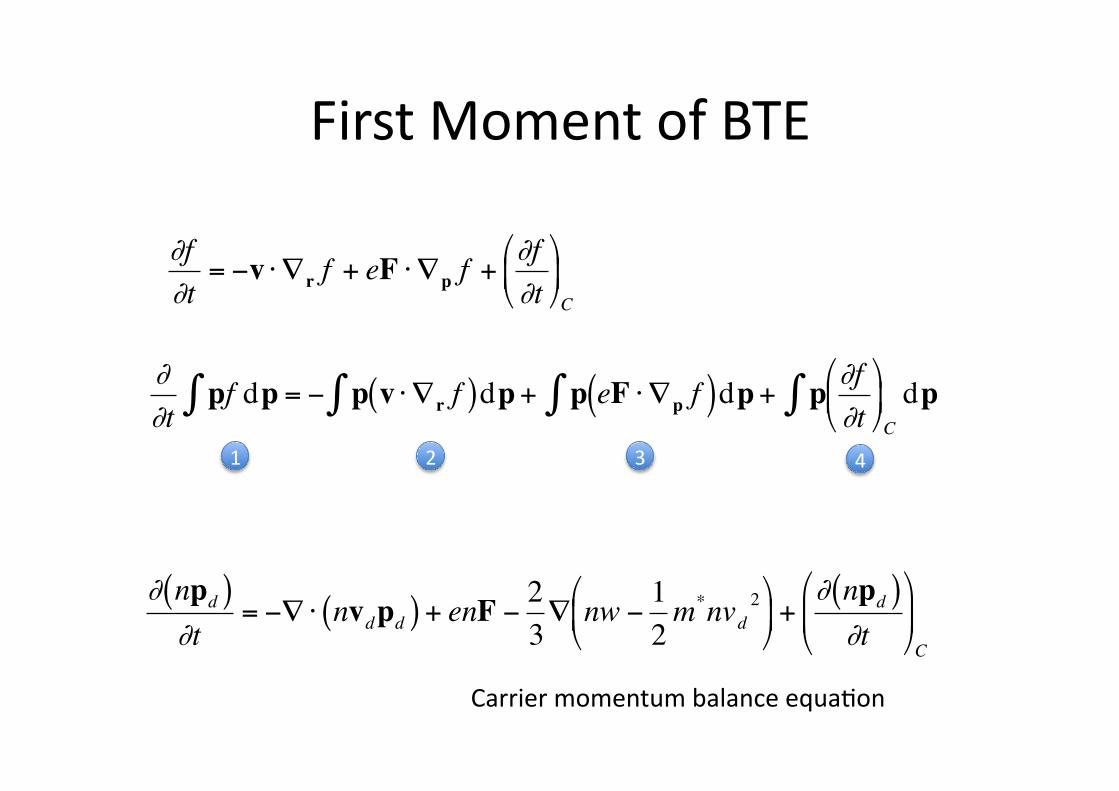
First Moment of BTE
€
∂f∂t
= −v ⋅ ∇ r f + eF ⋅ ∇p f +∂f∂t
C
€
∂∂t
pf dp∫ = − p v ⋅ ∇ r f( )dp∫ + p eF ⋅ ∇p f( )dp∫ + p ∂f∂t
C
dp∫1 2 3 4
€
∂ npd( )∂t
= −∇ ⋅ nvdpd( ) + enF − 23∇ nw − 1
2m*nvd
2
+
∂ npd( )∂t
C
Carrier momentum balance equa/on

Second Moment of BTE
€
∂f∂t
= −v ⋅ ∇ r f + eF ⋅ ∇p f +∂f∂t
C
€
∂∂t
wf dp∫ = − w v ⋅ ∇ r f( )dp∫ + w eF ⋅ ∇p f( )dp∫ + w ∂f∂t
C
dp∫1 2 3 4
€
∂ nw( )∂t
= −∇ ⋅ nvdw + vd nkBT + nq( ) + enF ⋅ vd +∂ nw( )∂t
C
Carrier energy balance equa/on

Termina/on Equa/on
To terminate the equa/on, we need an expression for the current. One simple choice is the drif‐diffusion current expression
€
∂n∂t
=∇ ⋅ n v( ) =∇ ⋅ nvd( ) =∇ ⋅ Jn
Carrier density balance equa/on.
momentum is introduced

Termina/on Equa/on
€
∂ nw( )∂t
= −∇ ⋅ nvdw + vd nkBT + nq( ) + enF ⋅ vd +∂ nw( )∂t
C
Carrier energy balance equa/on. €
∂ npd( )∂t
= −∇ ⋅ nvdpd( ) + enF − 23∇ nw − 1
2m*nvd
2
+
∂ npd( )∂t
C
Carrier momentum balance equa/on.
energy is introduced
heat flux is introduced
Termina/on equa/on needed, from some physical approxima/ons.

Balance Equa/ons
€
∂ npd( )∂t
= −∇ ⋅ nvdpd( ) + enF − 23∇ nw − 1
2m*nvd
2
+
∂ npd( )∂t
C
€
∂ nw( )∂t
= −∇ ⋅ nvdw + vd nkBT + nq( ) + enF ⋅ vd +∂ nw( )∂t
C
€
∂n∂t
=∇ ⋅ n v( ) =∇ ⋅ nvd( ) =∇ ⋅ Jn (1)
(2)
(3)
With appropriate termina/on equa/ons, ‐ We can solve eq (1) alone, which is our familiar Shockley con/nuity equa/on; or ‐ We can solve eq (1)‐(3), which are called the balance equa/ons.

Summary
• Microscopic and Macroscopic pictures – Equilibrium: • deriva/on of Boltzmann distribu/on
– Non‐equilibrium: • Boltzmann Transport Equa/on • Monte Carlo method
• Simplify BTE to obtain balance equa/ons