Embed Size (px)
Citation preview
Page 1
© R. Rutenbar 2001 CMU 18-760, Fall 2001 1
(Lec 12) ASIC Placement & Partitioning: (I)(Lec 12) ASIC Placement & Partitioning: (I)
What you know about layoutProbably not much, at this point...
What you don’t know about placement...Placement: which gates go where on the chip
Approaches: 3 big ideas here--recursive, iterative, & direct placement
ASICplacement
Gate-level netlistof placeable objects
and connecting wires
A “placement” ofthe gates in appropriate
location to “optimize” layout
© R. Rutenbar 2001 CMU 18-760, Fall 2001 2
Copyright NoticeCopyright Notice
© Rob A. Rutenbar 2001All rights reserved.You may not make copies of thismaterial in any form without myexpress permission.
Page 2
© R. Rutenbar 2001 CMU 18-760, Fall 2001 3
Where Are We?Where Are We?
Physical design--how to geometrically place gates in a netlist?
27 28 29 30 31 3 4 5 6 7
M T W Th F
10 11 12 13 14 17 18 19 20 21 24 25 26 27 28
AugSep
Oct 1 2 3 4 5 8 9 10 11 12
15 16 17 18 1922 23 24 25 26 29 30 31 1 2 5 6 7 8 9 Nov12 13 14 15 16 19 20 21 22 23 26 27 28 29 30 3 4 5 6 7
123456789101112131415
IntroductionAdvanced Boolean algebraJAVA ReviewFormal verification2-Level logic synthesisMulti-level logic synthesisTechnology mappingPlacementRoutingStatic timing analysisElectrical timing analysis Geometric data structs & apps
Dec
Thnxgive
10 11 12 13 14 16
Midsem break
© R. Rutenbar 2001 CMU 18-760, Fall 2001 4
HandoutsHandouts
PhysicalLecture 12 -- ASIC Placement & Partitioning
ElectronicNothing new...
Page 3
© R. Rutenbar 2001 CMU 18-760, Fall 2001 5
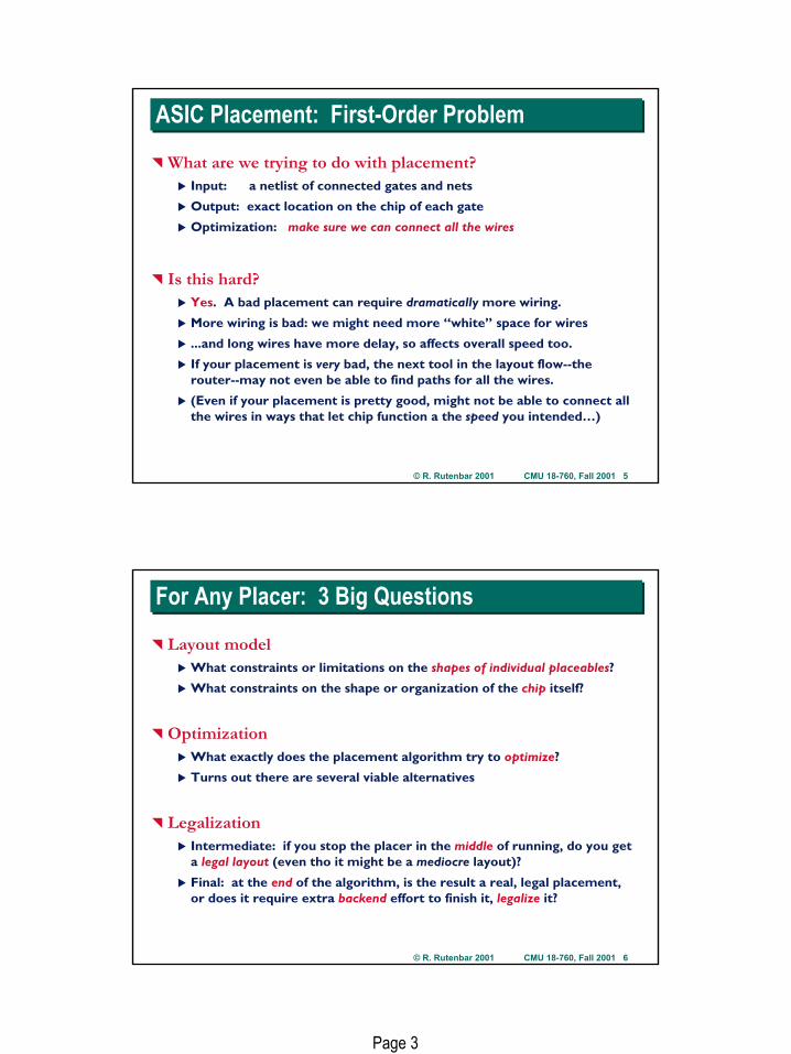
ASIC Placement: First-Order ProblemASIC Placement: First-Order Problem
What are we trying to do with placement?Input: a netlist of connected gates and nets
Output: exact location on the chip of each gate
Optimization: make sure we can connect all the wires
Is this hard?Yes. A bad placement can require dramatically more wiring.
More wiring is bad: we might need more “white” space for wires
...and long wires have more delay, so affects overall speed too.
If your placement is very bad, the next tool in the layout flow--the router--may not even be able to find paths for all the wires.
(Even if your placement is pretty good, might not be able to connect all the wires in ways that let chip function a the speed you intended…)
© R. Rutenbar 2001 CMU 18-760, Fall 2001 6
For Any Placer: 3 Big QuestionsFor Any Placer: 3 Big Questions
Layout modelWhat constraints or limitations on the shapes of individual placeables?
What constraints on the shape or organization of the chip itself?
OptimizationWhat exactly does the placement algorithm try to optimize?
Turns out there are several viable alternatives
LegalizationIntermediate: if you stop the placer in the middle of running, do you get a legal layout (even tho it might be a mediocre layout)?
Final: at the end of the algorithm, is the result a real, legal placement, or does it require extra backend effort to finish it, legalize it?
Page 4
© R. Rutenbar 2001 CMU 18-760, Fall 2001 7
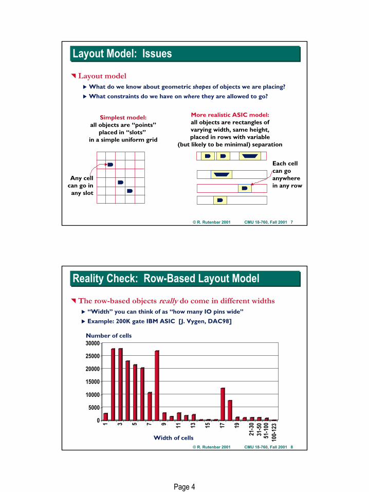
Layout Model: IssuesLayout Model: Issues
Layout modelWhat do we know about geometric shapes of objects we are placing?
What constraints do we have on where they are allowed to go?
Simplest model:all objects are “points”
placed in “slots” in a simple uniform grid
More realistic ASIC model:all objects are rectangles ofvarying width, same height,placed in rows with variable
(but likely to be minimal) separation
Any cellcan go in
any slot
Each cellcan goanywherein any row
© R. Rutenbar 2001 CMU 18-760, Fall 2001 8
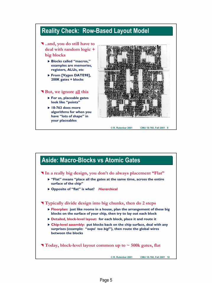
Reality Check: Row-Based Layout ModelReality Check: Row-Based Layout Model
The row-based objects really do come in different widths“Width” you can think of as “how many IO pins wide”
Example: 200K gate IBM ASIC [J. Vygen, DAC98]
0
5000
10000
15000
20000
25000
30000
1 3 5 7 9 11 13 15 17 19
21-3
0
51-1
00
Number of cells
Width of cells
31-5
0
100-
123
Page 5
© R. Rutenbar 2001 CMU 18-760, Fall 2001 9
Reality Check: Row-Based Layout ModelReality Check: Row-Based Layout Model
..and, you do still have to deal with random logic + big blocks
Blocks called “macros,” examples are memories, registers, ALUs, etc
From [Vygen DATE98], 200K gates + blocks
But, we ignore all thisFor us, placeable gates look like “points”
18-763 does more algorithms for when you have “lots of shape” in your placeables
© R. Rutenbar 2001 CMU 18-760, Fall 2001 10
Aside: Macro-Blocks vs Atomic GatesAside: Macro-Blocks vs Atomic Gates
In a really big design, you don’t do always placement “Flat”“Flat” means “place all the gates at the same time, across the entire surface of the chip”
Opposite of “flat” is what? Hierarchical
Typically divide design into big chunks, then do 2 stepsFloorplan: just like rooms in a house, plan the arrangement of these bigblocks on the surface of your chip, then try to lay out each block
Detailed, block-level layout: for each block, place it and route it
Chip-level assembly: put blocks back on the chip surface, deal with any surprises (example: “oops! too big!”), then route the global wires between the blocks
Today, block-level layout common up to ~ 500k gates, flat
Page 6
© R. Rutenbar 2001 CMU 18-760, Fall 2001 11
Aside: About FloorplansAside: About Floorplans
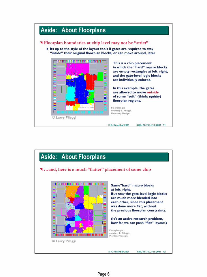
Floorplan boundaries at chip level may not be “strict”Its up to the style of the layout tools if gates are required to stay “inside” their original floorplan blocks, or can move around, later
© Larry Pileggi
Floorplan piccourtesy L. Pileggi,Monterey Design
This is a chip placementin which the “hard” macro blocksare empty rectangles at left, right, and the gate-level logic blocksare individually colored.
In this example, the gatesare allowed to move outsideof some “soft” (think: squishy)floorplan regions.
© R. Rutenbar 2001 CMU 18-760, Fall 2001 12
Aside: About FloorplansAside: About Floorplans
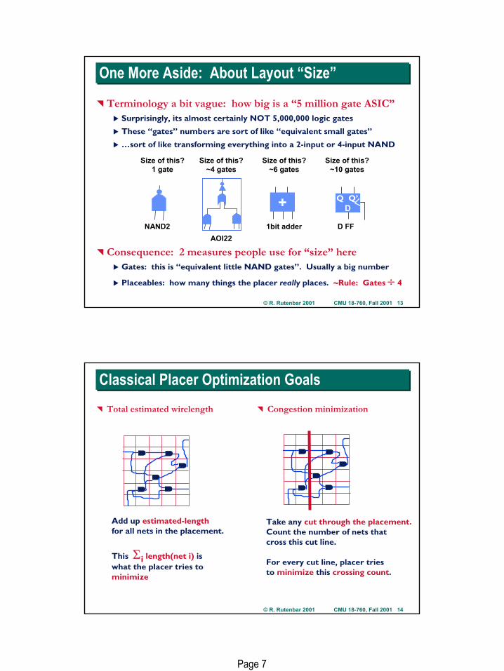
…and, here is a much “flatter” placement of same chip
© Larry Pileggi
Floorplan piccourtesy L. Pileggi,Monterey Design
Same“hard” macro blocksat left, right. But now the gate-level logic blocksare much more blended intoeach other, since this placementwas done more flat, withoutthe previous floorplan constraints.
(It’s an active research problem, how far we can push “flat” layout.)
Page 7
© R. Rutenbar 2001 CMU 18-760, Fall 2001 13
One More Aside: About Layout “Size”One More Aside: About Layout “Size”
Terminology a bit vague: how big is a “5 million gate ASIC”Surprisingly, its almost certainly NOT 5,000,000 logic gates
These “gates” numbers are sort of like “equivalent small gates”
…sort of like transforming everything into a 2-input or 4-input NAND
Consequence: 2 measures people use for “size” hereGates: this is “equivalent little NAND gates”. Usually a big number
Placeables: how many things the placer really places. ~Rule: Gates ÷ 4
Size of this?1 gate
+ D
D FF
Q Q’
Size of this?~6 gates
NAND2 1bit adder
Size of this?~10 gates
AOI22
Size of this?~4 gates
© R. Rutenbar 2001 CMU 18-760, Fall 2001 14
Classical Placer Optimization GoalsClassical Placer Optimization GoalsTotal estimated wirelength Congestion minimization
Add up estimated-lengthfor all nets in the placement.
This Σi length(net i) iswhat the placer tries tominimize
Take any cut through the placement.Count the number of nets thatcross this cut line.
For every cut line, placer triesto minimize this crossing count.
Page 8
© R. Rutenbar 2001 CMU 18-760, Fall 2001 15
Optimization: Minimum WirelengthOptimization: Minimum Wirelength
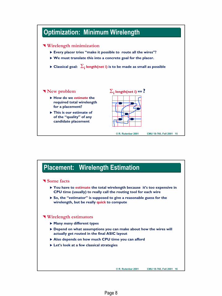
Wirelength minimizationEvery placer tries “make it possible to route all the wires”?
We must translate this into a concrete goal for the placer.
Classical goal: Σi length(net i) is to be made as small as possible
New problemHow do we estimate therequired total wirelengthfor a placement?
This is our estimate ofof the “quality” of anycandidate placement
Σi length(net i) == ?
© R. Rutenbar 2001 CMU 18-760, Fall 2001 16
Placement: Wirelength EstimationPlacement: Wirelength Estimation
Some factsYou have to estimate the total wirelength because it’s too expensive in CPU time (usually) to really call the routing tool for each wire
So, the “estimator” is supposed to give a reasonable guess for thewirelength, but be really quick to compute
Wirelength estimatorsMany many different types
Depend on what assumptions you can make about how the wires willactually get routed in the final ASIC layout
Also depends on how much CPU time you can afford
Let’s look at a few classical strategies
Page 9
© R. Rutenbar 2001 CMU 18-760, Fall 2001 17
Wirelength EstimationWirelength Estimation
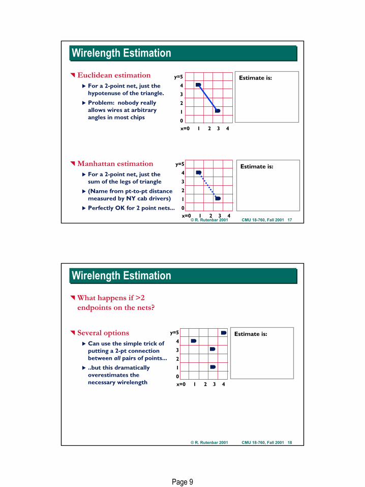
Euclidean estimationFor a 2-point net, just the hypotenuse of the triangle.
Problem: nobody reallyallows wires at arbitraryangles in most chips
Manhattan estimationFor a 2-point net, just thesum of the legs of triangle
(Name from pt-to-pt distancemeasured by NY cab drivers)
Perfectly OK for 2 point nets...
Estimate is:
Estimate is:
x=0 1 2 3 4
y=5
4
3
2
1
0
x=0 1 2 3 4
y=5
4
3
2
1
0
© R. Rutenbar 2001 CMU 18-760, Fall 2001 18
Wirelength EstimationWirelength Estimation
What happens if >2 endpoints on the nets?
Several optionsCan use the simple trick of putting a 2-pt connection between all pairs of points...
..but this dramatically overestimates the necessary wirelength
Estimate is:
x=0 1 2 3 4
y=5
4
3
2
1
0
Page 10
© R. Rutenbar 2001 CMU 18-760, Fall 2001 19
Wirelength EstimationWirelength Estimation
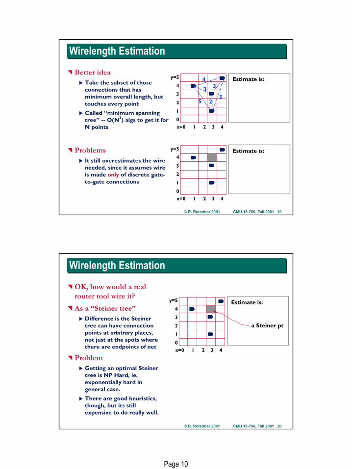
Better ideaTake the subset of those connections that has minimum overall length, but touches every point
Called “minimum spanning tree” -- O(N2) algs to get it for N points
ProblemsIt still overestimates the wire needed, since it assumes wire is made only of discrete gate-to-gate connections
Estimate is:
x=0 1 2 3 4
y=5
4
3
2
1
0
4
55
2
3 3
Estimate is:
x=0 1 2 3 4
y=5
4
3
2
1
0
© R. Rutenbar 2001 CMU 18-760, Fall 2001 20
Wirelength EstimationWirelength Estimation
OK, how would a real router tool wire it?
As a “Steiner tree”Difference is the Steiner tree can have connection points at arbitrary places, not just at the spots where there are endpoints of net
ProblemGetting an optimal Steiner tree is NP Hard, ie, exponentially hard in general case.
There are good heuristics, though, but its still expensive to do really well.
Estimate is:
x=0 1 2 3 4
y=5
4
3
2
1
0
a Steiner pt
Page 11
© R. Rutenbar 2001 CMU 18-760, Fall 2001 21
Aside: About Steiner Tree Constructions Aside: About Steiner Tree Constructions
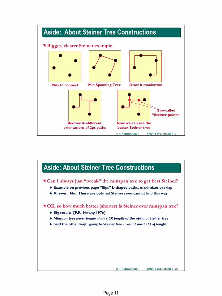
Bigger, clearer Steiner example
Pins to connect Min Spanning Tree Draw it manhattan
Redraw it--differentorientations of 2pt paths
Now we can see thebetter Steiner tree
2 so-called“Steiner-points”
© R. Rutenbar 2001 CMU 18-760, Fall 2001 22
Aside: About Steiner Tree ConstructionsAside: About Steiner Tree Constructions
Can I always just “tweak” the minspan tree to get best Steiner?Example on previous page “flips” L-shaped paths, maximizes overlap
Answer: No. There are optimal Steiners you cannot find this way
OK, so how much better (shorter) is Steiner over minspan tree?Big result: [F.K. Hwang 1976]
Minspan tree never longer than 1.5X length of the optimal Steiner tree
Said the other way: going to Steiner tree saves at most 1/3 of length
Page 12
© R. Rutenbar 2001 CMU 18-760, Fall 2001 23
Wirelength EstimationWirelength Estimation
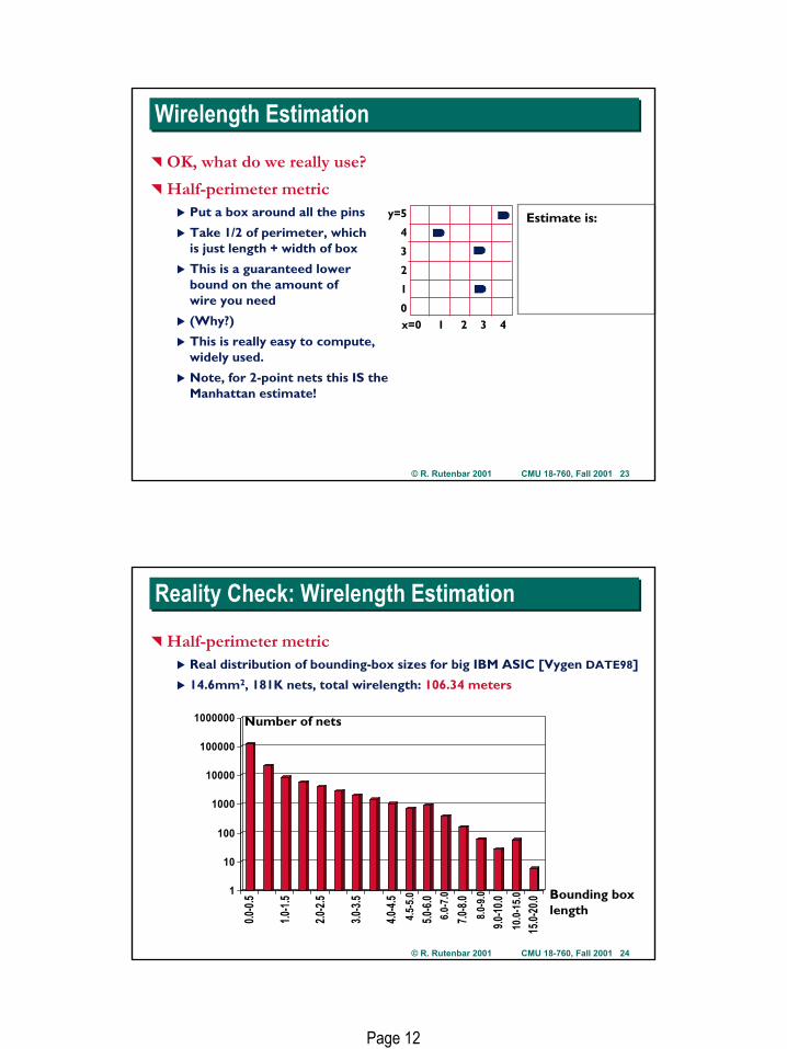
OK, what do we really use?
Half-perimeter metricPut a box around all the pins
Take 1/2 of perimeter, which is just length + width of box
This is a guaranteed lower bound on the amount of wire you need
(Why?)
This is really easy to compute, widely used.
Note, for 2-point nets this IS the Manhattan estimate!
Estimate is:
x=0 1 2 3 4
y=5
4
3
2
1
0
© R. Rutenbar 2001 CMU 18-760, Fall 2001 24
Reality Check: Wirelength EstimationReality Check: Wirelength Estimation
Half-perimeter metricReal distribution of bounding-box sizes for big IBM ASIC [Vygen DATE98]
14.6mm2, 181K nets, total wirelength: 106.34 meters
1
10
100
1000
10000
100000
1000000
0.0-0.
5
1.0-1.
5
2.0-2.
5
3.0-3.
5
4.0-4.
5
5.0-6.
0
7.0-8.
0
9.0-10
.0
15.0-
20.0
6.0-7
.0
8.0-9
.0
10.0-
15.0
Number of nets
Bounding boxlength4.5
-5.0
Page 13
© R. Rutenbar 2001 CMU 18-760, Fall 2001 25
Optimization: Congestion MinimizationOptimization: Congestion Minimization
Wirelength minimization is not only optionSmall total wirelength is good: shorter wires take up less space, have less delay, etc
BUT--still easy to place too many gates so close you cannot wire them
Estimated wirelength does not account for congestion, ie, there is more demand for wires than supply of wires in a region of space
Can target congestion instead of wirelengthNote they do tend to correlate, but minimizing one does not neccessarily optimize the other
© R. Rutenbar 2001 CMU 18-760, Fall 2001 26
Congestion vs WirelengthCongestion vs Wirelength
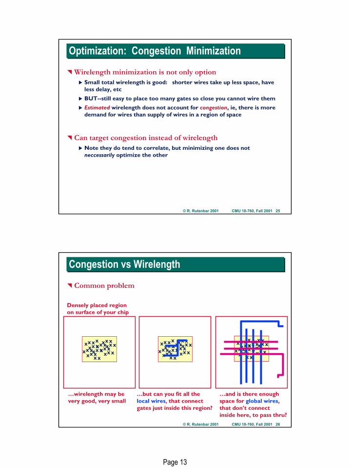
Common problem
xx
x
xx
xx
xxx
x
x
xx
xx
xx
xx
xx
xxx
xx
xx
xx
xx
xx
x
xx
xx
xxx
x
x
xx
xx
xx
xx
xx
xxx
xx
xx
xx
xx
xx
x
xx
xx
xxx
x
x
xx
xx
xx
xx
xx
xxx
xx
xx
xx
xx
Densely placed regionon surface of your chip
…wirelength may bevery good, very small
…but can you fit all thelocal wires, that connectgates just inside this region?
…and is there enough space for global wires, that don’t connectinside here, to pass thru?
Page 14
© R. Rutenbar 2001 CMU 18-760, Fall 2001 27
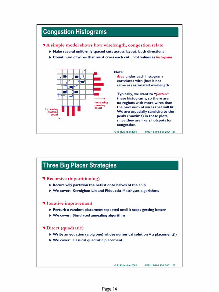
Congestion HistogramsCongestion Histograms
A simple model shows how wirelength, congestion relateMake several uniformly spaced cuts across layout, both directions
Count num of wires that must cross each cut; plot values as histogram
Note:Area under each histogram correlates with (but is notsame as) estimated wirelength
Typically, we want to “flatten”these histograms, so there areno regions with more wires thanthe max num of wires that will fit.We are especially sensitive to thepeaks (maxima) in these plots, since they are likely hotspots forcongestion.
IncreasingcrossingcountIncreasing
crossingcount
© R. Rutenbar 2001 CMU 18-760, Fall 2001 28
Three Big Placer StrategiesThree Big Placer Strategies
Recursive (bipartitioning)Recursively partition the netlist onto halves of the chip
We cover: Kernighan-Lin and Fidduccia-Matthyses algorithms
Iterative improvementPerturb a random placement repeated until it stops getting better
We cover: Simulated annealing algorithm
Direct (quadratic)Write an equation (a big one) whose numerical solution = a placement(!)
We cover: classical quadratic placement
Page 15
© R. Rutenbar 2001 CMU 18-760, Fall 2001 29
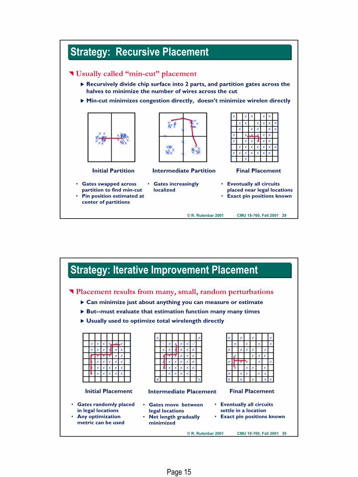
Strategy: Recursive PlacementStrategy: Recursive Placement
Usually called “min-cut” placementRecursively divide chip surface into 2 parts, and partition gates across the halves to minimize the number of wires across the cut
Min-cut minimizes congestion directly, doesn’t minimize wirelen directly
Initial Partition
• Gates swapped across partition to find min-cut
• Pin position estimated at center of partitions
Intermediate Partition
• Gates increasingly localized
Final Placement
• Eventually all circuits placed near legal locations
• Exact pin positions known
© R. Rutenbar 2001 CMU 18-760, Fall 2001 30
Strategy: Iterative Improvement PlacementStrategy: Iterative Improvement Placement
Placement results from many, small, random perturbationsCan minimize just about anything you can measure or estimate
But--must evaluate that estimation function many many times
Usually used to optimize total wirelength directly
Initial Placement
• Gates randomly placed in legal locations
• Any optimizationmetric can be used
Final Placement
• Eventually all circuits settle in a location
• Exact pin positions known
Intermediate Placement
• Gates move between legal locations
• Net length gradually minimized
Page 16
© R. Rutenbar 2001 CMU 18-760, Fall 2001 31
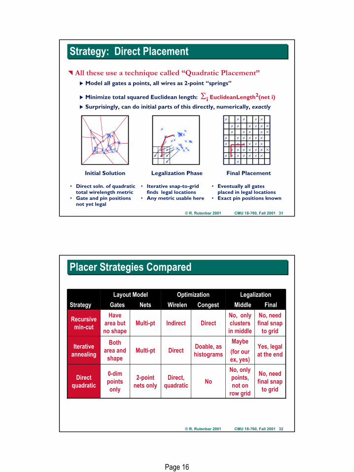
Strategy: Direct PlacementStrategy: Direct Placement
All these use a technique called “Quadratic Placement”Model all gates a points, all wires as 2-point “springs”
Minimize total squared Euclidean length: Σi EuclideanLength2(net i)
Surprisingly, can do initial parts of this directly, numerically, exactly
Initial Solution
• Direct soln. of quadratic total wirelength metric
• Gate and pin positions not yet legal
Legalization Phase
• Iterative snap-to-grid finds legal locations
• Any metric usable here
Final Placement
• Eventually all gates placed in legal locations
• Exact pin positions known
© R. Rutenbar 2001 CMU 18-760, Fall 2001 32
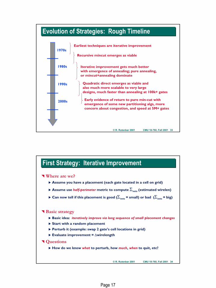
Placer Strategies Compared Placer Strategies Compared
Yes, legal at the end
Maybe(for our ex, yes)
Doable, as histogramsDirectMulti-pt
Both area and
shape
Iterativeannealing
No, need final snap
to grid
No, only points, not on
row grid
NoDirect, quadratic
2-point nets only
0-dim points only
Direct quadratic
No, need final snap
to grid
No, only clusters in middle
DirectIndirectMulti-ptHave
area but no shape
Recursive min-cut
LegalizationMiddle Final
OptimizationWirelen Congest
Layout ModelGates NetsStrategy
Page 17
© R. Rutenbar 2001 CMU 18-760, Fall 2001 33
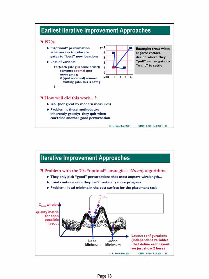
Evolution of Strategies: Rough TimelineEvolution of Strategies: Rough Timeline
1970s
1980s
1990s
2000s
Earliest techniques are iterative improvement
Recursive mincut emerges as viable
Iterative improvement gets much betterwith emergence of annealing; pure annealing, or mincut+annealing dominate
Quadratic direct emerges as viable andalso much more scalable to very largedesigns, much faster than annealing at 100k+ gates
Early evidence of return to pure min-cut withemergence of some new partitioning algs, moreconcern about congestion, and speed at 5M+ gates
© R. Rutenbar 2001 CMU 18-760, Fall 2001 34
First Strategy: Iterative ImprovementFirst Strategy: Iterative Improvement
Where are we?Assume you have a placement (each gate located in a cell on grid)
Assume use half-perimeter metric to compute Σnets (estimated wirelen)
Can now tell if this placement is good (Σnets = small) or bad (Σnets = big)
Basic strategyBasic idea: iteratively improve via long sequence of small placement changes
Start with a random placement
Perturb it (example: swap 2 gate’s cell locations in grid)
Evaluate improvement = ∆wirelength
QuestionsHow do we know what to perturb, how much, when to quit, etc?
Page 18
© R. Rutenbar 2001 CMU 18-760, Fall 2001 35
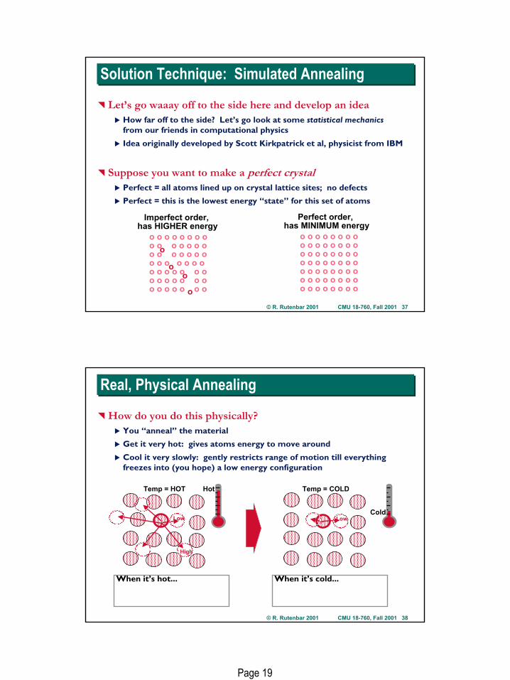
Earliest Iterative Improvement ApproachesEarliest Iterative Improvement Approaches1970s
“Optimal” perturbation schemes try to relocate gates to “best” new locations
Lots of variantsFor(each gate g in some order){
compute optimal spotmove gate gif (spot occupied) remove
existing gate, this is new g
}
How well did this work…?OK (not great by modern measures)
Problem is these methods are inherently greedy: they quit when can’t find another good perturbation
Example: treat wiresas force vectors,decide where they“pull” center gate to“want” to settle
x=0 1 2 3 4
y=5
4
3
2
1
0
© R. Rutenbar 2001 CMU 18-760, Fall 2001 36
Iterative Improvement ApproachesIterative Improvement Approaches
Problem with the 70s “optimal” strategies: Greedy algorithmsThey only pick “good” perturbations that most improve wirelength...
...and continue until they can’t make any more progress
Problem: local minima in the cost surface for the placement task
Σnets wirelen
quality metricfor eachpossible
layout
LocalMinimum
GlobalMinimum
Layout configurations(independent variablesthat define each layout;
we just show 2 here)
Page 19
© R. Rutenbar 2001 CMU 18-760, Fall 2001 37
Solution Technique: Simulated AnnealingSolution Technique: Simulated Annealing
Let’s go waaay off to the side here and develop an ideaHow far off to the side? Let’s go look at some statistical mechanics from our friends in computational physics
Idea originally developed by Scott Kirkpatrick et al, physicist from IBM
Suppose you want to make a perfect crystalPerfect = all atoms lined up on crystal lattice sites; no defects
Perfect = this is the lowest energy “state” for this set of atoms
o o o o o o o oo o o o o o oo o o o o o oo o o o o o oo o o o o o oo o o o o o oo o o o o o o
o o o o o o o oo o o o o o o oo o o o o o o oo o o o o o o oo o o o o o o oo o o o o o o oo o o o o o o o
o
oo
o
Imperfect order, has HIGHER energy
Perfect order, has MINIMUM energy
© R. Rutenbar 2001 CMU 18-760, Fall 2001 38
Real, Physical AnnealingReal, Physical Annealing
How do you do this physically?You “anneal” the material
Get it very hot: gives atoms energy to move around
Cool it very slowly: gently restricts range of motion till everything freezes into (you hope) a low energy configuration
Temp = HOT
Low
High
Hot Temp = COLD
LowCold
When it’s hot... When it’s cold...
Page 20
© R. Rutenbar 2001 CMU 18-760, Fall 2001 39
Annealing -> Simulated AnnealingAnnealing -> Simulated Annealing
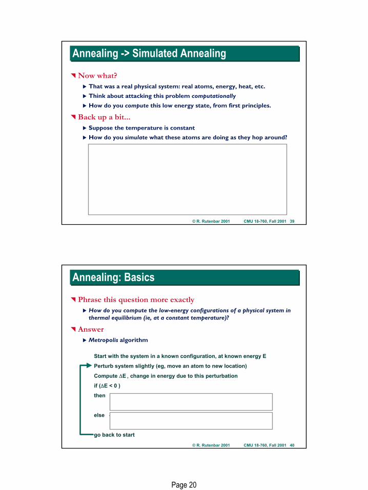
Now what?That was a real physical system: real atoms, energy, heat, etc.
Think about attacking this problem computationally
How do you compute this low energy state, from first principles.
Back up a bit...Suppose the temperature is constant
How do you simulate what these atoms are doing as they hop around?
© R. Rutenbar 2001 CMU 18-760, Fall 2001 40
Annealing: BasicsAnnealing: Basics
Phrase this question more exactlyHow do you compute the low-energy configurations of a physical system in thermal equilibrium (ie, at a constant temperature)?
AnswerMetropolis algorithm
Start with the system in a known configuration, at known energy E
Perturb system slightly (eg, move an atom to new location)
Compute ∆E , change in energy due to this perturbation
if (∆E < 0 )
then
else {
go back to start
Page 21
© R. Rutenbar 2001 CMU 18-760, Fall 2001 41
Aside: Metropolis CriterionAside: Metropolis Criterion
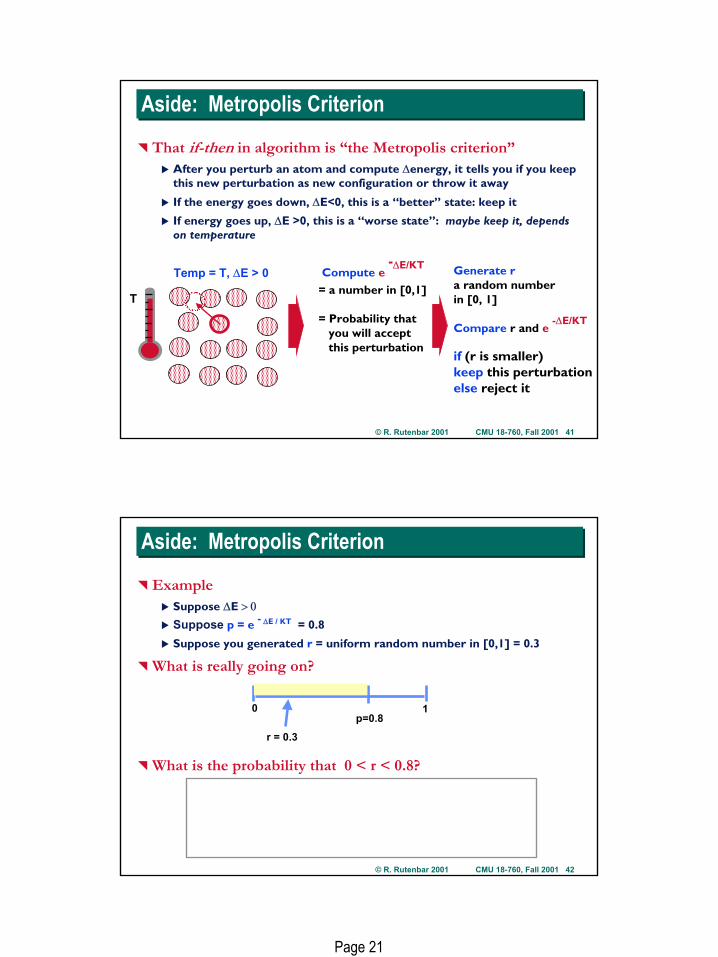
That if-then in algorithm is “the Metropolis criterion”After you perturb an atom and compute ∆energy, it tells you if you keep this new perturbation as new configuration or throw it away
If the energy goes down, ∆E<0, this is a “better” state: keep it
If energy goes up, ∆E >0, this is a “worse state”: maybe keep it, depends on temperature
Temp = T, ∆E > 0
T
Compute e -∆E/KT
= a number in [0,1]
= Probability thatyou will accept this perturbation
Generate ra random numberin [0, 1]
Compare r and e -∆E/KT
if (r is smaller)keep this perturbationelse reject it
© R. Rutenbar 2001 CMU 18-760, Fall 2001 42
Aside: Metropolis CriterionAside: Metropolis Criterion
ExampleSuppose ∆E > 0
Suppose p = e - ∆E / KT = 0.8
Suppose you generated r = uniform random number in [0,1] = 0.3
What is really going on?
What is the probability that 0 < r < 0.8?
0 1p=0.8
r = 0.3
Page 22
© R. Rutenbar 2001 CMU 18-760, Fall 2001 43
Simulated AnnealingSimulated Annealing
QuestionMetropolis algorithm iteratively visits configurations with “reasonably probable” energies at the given fixed temperature
What if I want to find a minimum energy state, now what do I do?
AnswerSimulated annealing
Add outer loop that starts with a high temperature, and slowly cools it
Do enough perturbations at each temperature in the sequence of cooling steps to get to thermal equilibrium (ie, do the Metropolis procedure)
Do enough temperatures so that the problem actually freezes into a low energy state, and further cooling does not further lower energy
© R. Rutenbar 2001 CMU 18-760, Fall 2001 44
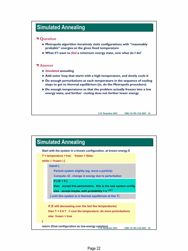
Simulated Annealing Simulated Annealing Start with the system in a known configuration, at known energy E
T = temperature = hot; frozen = false;
while ( ! frozen ) {
repeat {
Perturb system slightly (eg, move a particle)
Compute ∆E , change in energy due to perturbation
if (∆E < 0 )
then accept this perturbation, this is the new system config
else accept maybe, with probability = e -∆E/T
} until (the system is in thermal equilibrium at this T)
If (E still decreasing over the last few temperatures)
then T = 0.9 T // cool the temperature; do more perturbations
else frozen = true
}
return (final configuration as low-energy solution)
Page 23
© R. Rutenbar 2001 CMU 18-760, Fall 2001 45
Toy ExampleToy Example
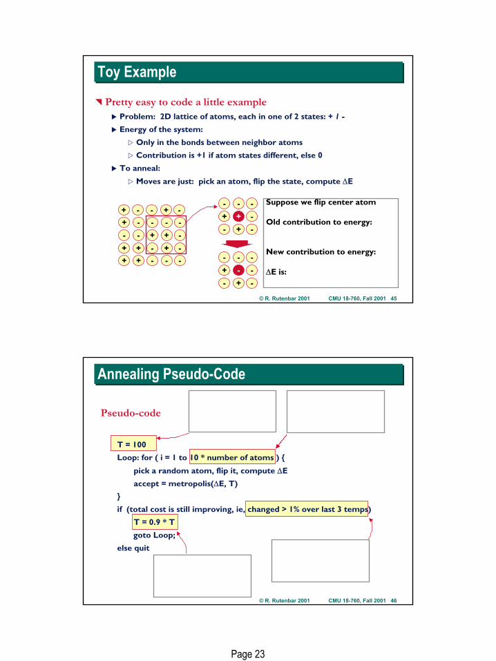
Pretty easy to code a little exampleProblem: 2D lattice of atoms, each in one of 2 states: + 1 -
Energy of the system:
Only in the bonds between neighbor atoms
Contribution is +1 if atom states different, else 0
To anneal:
Moves are just: pick an atom, flip the state, compute ∆E
+ - - + -
+ - - - -
- - + + -
+ + - + -
+ + - - -
- - -
+ + -
- + -
Suppose we flip center atom
Old contribution to energy:
New contribution to energy:
∆E is:
- - -
+ - -
- + -
© R. Rutenbar 2001 CMU 18-760, Fall 2001 46
Annealing Pseudo-CodeAnnealing Pseudo-Code
Pseudo-code
T = 100
Loop: for ( i = 1 to 10 * number of atoms ) {
pick a random atom, flip it, compute ∆E
accept = metropolis(∆E, T)
}
if (total cost is still improving, ie, changed > 1% over last 3 temps)
T = 0.9 * T
goto Loop;
else quit
Page 24
© R. Rutenbar 2001 CMU 18-760, Fall 2001 47
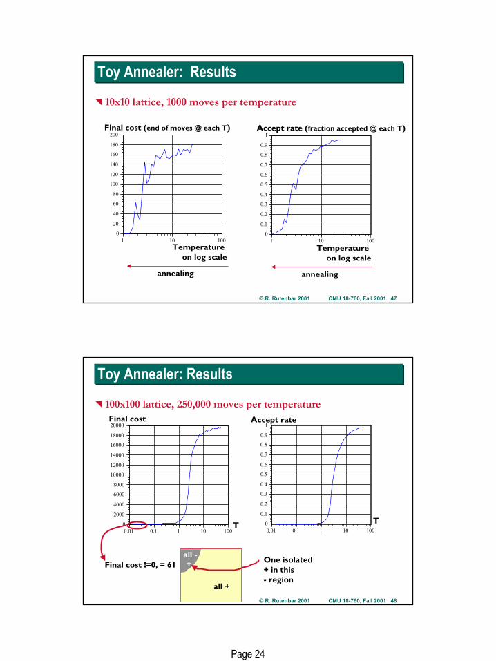
Toy Annealer: ResultsToy Annealer: Results
10x10 lattice, 1000 moves per temperature
0
20
40
60
80
100
120
140
160
180
200
1 10 1000
0.1
0.2
0.3
0.4
0.5
0.6
0.7
0.8
0.9
1
1 10 100
Final cost (end of moves @ each T)
Temperature on log scale
annealing
Temperature on log scale
annealing
Accept rate (fraction accepted @ each T)
© R. Rutenbar 2001 CMU 18-760, Fall 2001 48
Toy Annealer: ResultsToy Annealer: Results
100x100 lattice, 250,000 moves per temperature
0
2000
4000
6000
8000
10000
12000
14000
16000
18000
20000
0.01 0.1 1 10 1000
0.1
0.2
0.3
0.4
0.5
0.6
0.7
0.8
0.9
1
0.01 0.1 1 10 100
Final cost
T
Accept rate
T
Final cost !=0, = 61
all +
all -+ One isolated
+ in this- region
Page 25
© R. Rutenbar 2001 CMU 18-760, Fall 2001 49
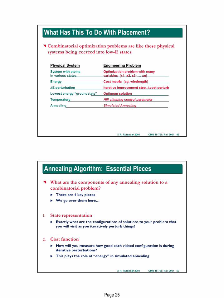
What Has This To Do With Placement?What Has This To Do With Placement?
Combinatorial optimization problems are like these physical systems being coerced into low-E states
Physical System Engineering ProblemSystem with atoms Optimization problem with manyin various states variables (x1, x2, x3, ..., xn)
Energy Cost metric (eg, wirelength)
∆E perturbation Iterative improvement step, ∆cost perturb
Lowest energy “groundstate” Optimum solution
Temperature Hill climbing control parameter
Annealing Simulated Annealing
© R. Rutenbar 2001 CMU 18-760, Fall 2001 50
Annealing Algorithm: Essential PiecesAnnealing Algorithm: Essential Pieces
What are the components of any annealing solution to a combinatorial problem?
There are 4 key pieces
We go over them here…
1. State representationExactly what are the configurations of solutions to your problem that you will visit as you iteratively perturb things?
2. Cost functionHow will you measure how good each visited configuration is during iterative perturbations?
This plays the role of “energy” in simulated annealing
Page 26
© R. Rutenbar 2001 CMU 18-760, Fall 2001 51
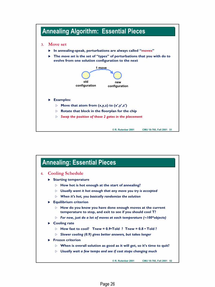
Annealing Algorithm: Essential PiecesAnnealing Algorithm: Essential Pieces
3. Move setIn annealing-speak, perturbations are always called “moves”
The move set is the set of “types” of perturbations that you with do to evolve from one solution configuration to the next
Examples:
Move that atom from (x,y,z) to (x’,y’,z’)
Rotate that block in the floorplan for the chip
Swap the position of those 2 gates in the placement
oldconfiguration
newconfiguration
1 move
© R. Rutenbar 2001 CMU 18-760, Fall 2001 52
Annealing: Essential PiecesAnnealing: Essential Pieces4. Cooling Schedule
Starting temperature
How hot is hot enough at the start of annealing?
Usually want it hot enough that any move you try is accepted
When it’s hot, you basically randomize the solution
Equilibrium criterion
How do you know you have done enough moves at the current temperature to stop, and exit to see if you should cool T?
For now, just do a lot of moves at each temperature (~100*objects)
Cooling rate
How fast to cool? Tnew = 0.9•Told ? Tnew = 0.8 • Told ?
Slower cooling (0.9) gives better answers, but takes longer
Frozen criterion
When is overall solution as good as it will get, so it’s time to quit?
Usually wait a few temps and see if cost stops changing much
Page 27
© R. Rutenbar 2001 CMU 18-760, Fall 2001 53
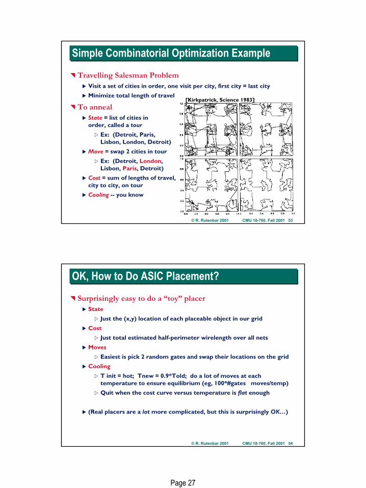
Simple Combinatorial Optimization ExampleSimple Combinatorial Optimization Example
Travelling Salesman ProblemVisit a set of cities in order, one visit per city, first city = last city
Minimize total length of travel
To annealState = list of cities inorder, called a tour
Ex: (Detroit, Paris, Lisbon, London, Detroit)
Move = swap 2 cities in tour
Ex: (Detroit, London,Lisbon, Paris, Detroit)
Cost = sum of lengths of travel,city to city, on tour
Cooling -- you know
[Kirkpatrick, Science 1983]
© R. Rutenbar 2001 CMU 18-760, Fall 2001 54
OK, How to Do ASIC Placement?OK, How to Do ASIC Placement?
Surprisingly easy to do a “toy” placerState
Just the (x,y) location of each placeable object in our grid
Cost
Just total estimated half-perimeter wirelength over all nets
Moves
Easiest is pick 2 random gates and swap their locations on the grid
Cooling
T init = hot; Tnew = 0.9*Told; do a lot of moves at each temperature to ensure equilibrium (eg, 100*#gates moves/temp)
Quit when the cost curve versus temperature is flat enough
(Real placers are a lot more complicated, but this is surprisingly OK…)
Page 28
© R. Rutenbar 2001 CMU 18-760, Fall 2001 55
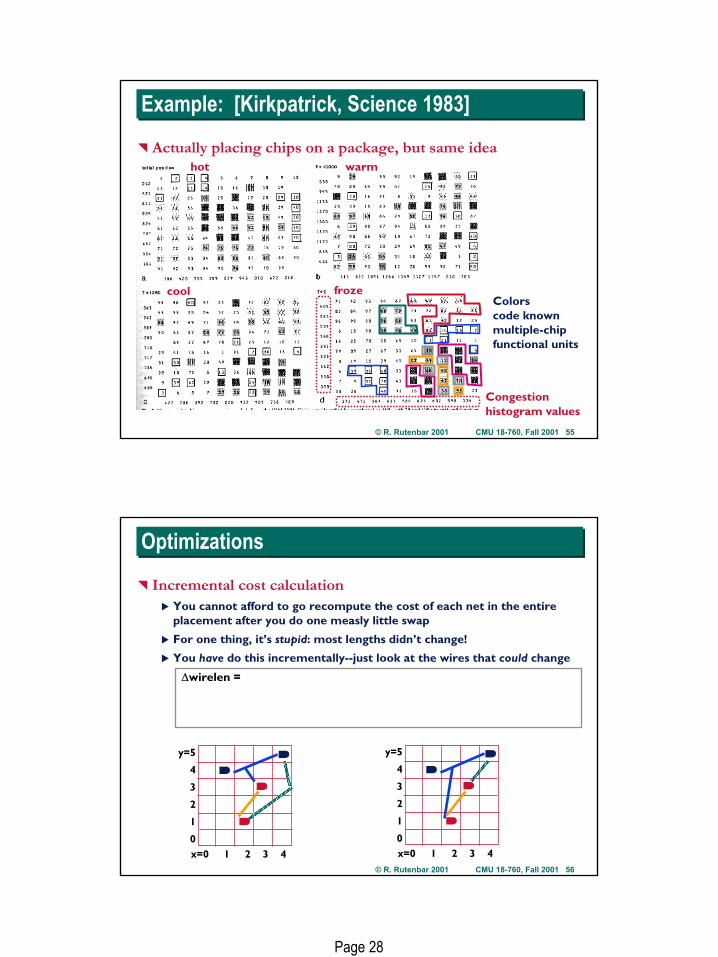
Example: [Kirkpatrick, Science 1983]Example: [Kirkpatrick, Science 1983]
Actually placing chips on a package, but same ideahot warm
cool froze
Congestionhistogram values
Colorscode knownmultiple-chipfunctional units
© R. Rutenbar 2001 CMU 18-760, Fall 2001 56
OptimizationsOptimizations
Incremental cost calculationYou cannot afford to go recompute the cost of each net in the entire placement after you do one measly little swap
For one thing, it’s stupid: most lengths didn’t change!
You have do this incrementally--just look at the wires that could change
x=0 1 2 3 4
y=5
4
3
2
1
0
∆wirelen =
x=0 1 2 3 4
y=5
4
3
2
1
0
Page 29
© R. Rutenbar 2001 CMU 18-760, Fall 2001 57
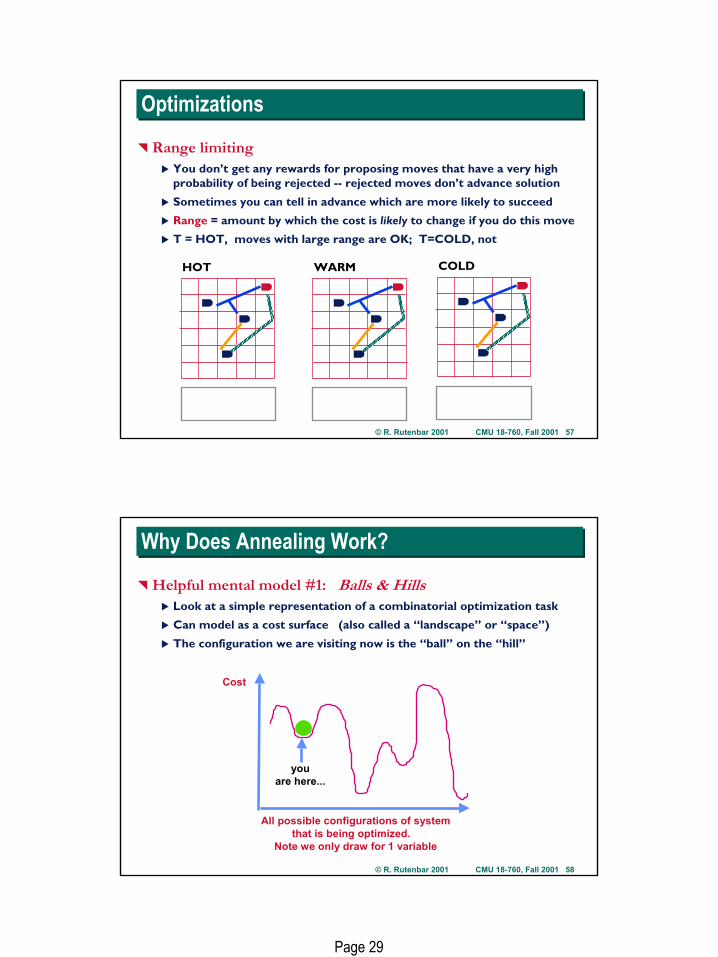
OptimizationsOptimizations
Range limitingYou don’t get any rewards for proposing moves that have a very high probability of being rejected -- rejected moves don’t advance solution
Sometimes you can tell in advance which are more likely to succeed
Range = amount by which the cost is likely to change if you do this move
T = HOT, moves with large range are OK; T=COLD, not
HOT WARM COLD
© R. Rutenbar 2001 CMU 18-760, Fall 2001 58
Why Does Annealing Work?Why Does Annealing Work?
Helpful mental model #1: Balls & HillsLook at a simple representation of a combinatorial optimization task
Can model as a cost surface (also called a “landscape” or “space”)
The configuration we are visiting now is the “ball” on the “hill”
Cost
All possible configurations of systemthat is being optimized.
Note we only draw for 1 variable
youare here...
Page 30
© R. Rutenbar 2001 CMU 18-760, Fall 2001 59
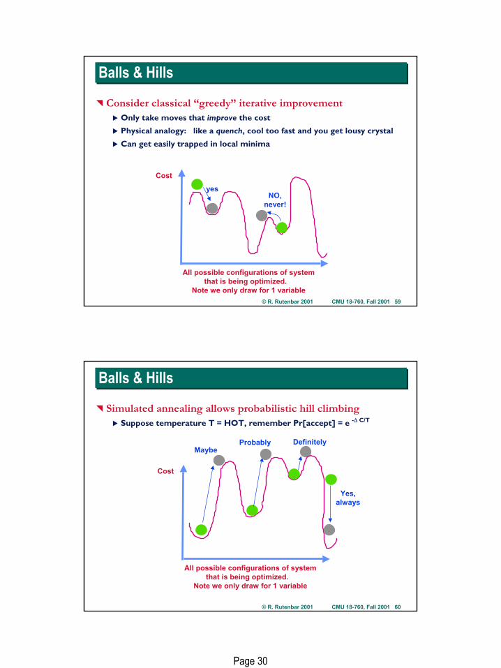
Balls & HillsBalls & Hills
Consider classical “greedy” iterative improvementOnly take moves that improve the cost
Physical analogy: like a quench, cool too fast and you get lousy crystal
Can get easily trapped in local minima
Cost
All possible configurations of systemthat is being optimized.
Note we only draw for 1 variable
yesNO,
never!
© R. Rutenbar 2001 CMU 18-760, Fall 2001 60
Balls & HillsBalls & Hills
Simulated annealing allows probabilistic hill climbingSuppose temperature T = HOT, remember Pr[accept] = e -∆ C/T
Cost
All possible configurations of systemthat is being optimized.
Note we only draw for 1 variable
MaybeProbably Definitely
Yes,always
Page 31
© R. Rutenbar 2001 CMU 18-760, Fall 2001 61
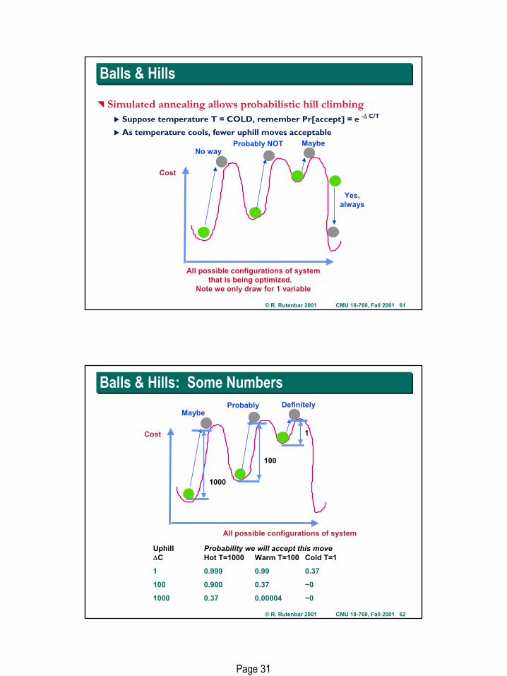
Balls & HillsBalls & Hills
Simulated annealing allows probabilistic hill climbingSuppose temperature T = COLD, remember Pr[accept] = e -∆ C/T
As temperature cools, fewer uphill moves acceptable
Cost
All possible configurations of systemthat is being optimized.
Note we only draw for 1 variable
No wayProbably NOT Maybe
Yes,always
© R. Rutenbar 2001 CMU 18-760, Fall 2001 62
Balls & Hills: Some NumbersBalls & Hills: Some Numbers
Cost
All possible configurations of system
MaybeProbably Definitely
1000
100
1
Uphill Probability we will accept this move∆C Hot T=1000 Warm T=100 Cold T=1
1 0.999 0.99 0.37
100 0.900 0.37 ~0
1000 0.37 0.00004 ~0
Page 32
© R. Rutenbar 2001 CMU 18-760, Fall 2001 63
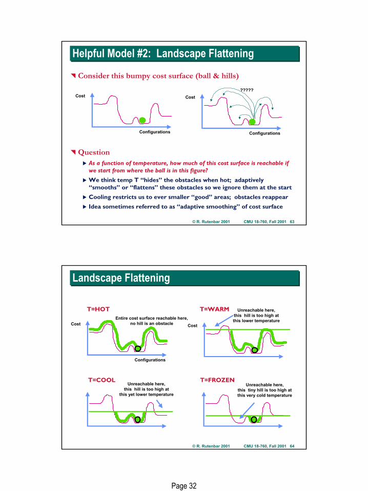
Helpful Model #2: Landscape FlatteningHelpful Model #2: Landscape Flattening
Consider this bumpy cost surface (ball & hills)
QuestionAs a function of temperature, how much of this cost surface is reachable if we start from where the ball is in this figure?
We think temp T “hides” the obstacles when hot; adaptively “smooths” or “flattens” these obstacles so we ignore them at the start
Cooling restricts us to ever smaller “good” areas; obstacles reappear
Idea sometimes referred to as “adaptive smoothing” of cost surface
Cost
Configurations
Cost
Configurations
?????
© R. Rutenbar 2001 CMU 18-760, Fall 2001 64
Landscape FlatteningLandscape Flattening
Cost
Unreachable here,this hill is too high atthis lower temperature
Unreachable here,this hill is too high at
this yet lower temperature
Unreachable here,this tiny hill is too high atthis very cold temperature
Cost
Configurations
Entire cost surface reachable here,no hill is an obstacle
T=HOT T=WARM
T=COOL T=FROZEN
Page 33
© R. Rutenbar 2001 CMU 18-760, Fall 2001 65
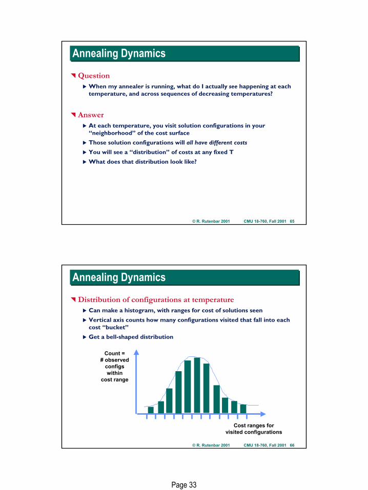
Annealing DynamicsAnnealing Dynamics
QuestionWhen my annealer is running, what do I actually see happening at each temperature, and across sequences of decreasing temperatures?
AnswerAt each temperature, you visit solution configurations in your “neighborhood” of the cost surface
Those solution configurations will all have different costs
You will see a “distribution” of costs at any fixed T
What does that distribution look like?
© R. Rutenbar 2001 CMU 18-760, Fall 2001 66
Annealing DynamicsAnnealing Dynamics
Distribution of configurations at temperatureCan make a histogram, with ranges for cost of solutions seen
Vertical axis counts how many configurations visited that fall into each cost “bucket”
Get a bell-shaped distribution
Count =# observed
configswithin
cost range
Cost ranges forvisited configurations
Page 34
© R. Rutenbar 2001 CMU 18-760, Fall 2001 67
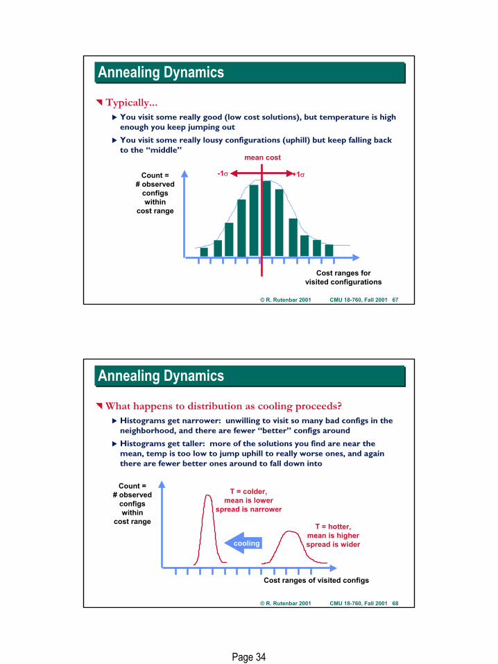
Annealing DynamicsAnnealing Dynamics
Typically...You visit some really good (low cost solutions), but temperature is high enough you keep jumping out
You visit some really lousy configurations (uphill) but keep falling back to the “middle”
Count =# observed
configswithin
cost range
Cost ranges forvisited configurations
mean cost
+1σ-1σ
© R. Rutenbar 2001 CMU 18-760, Fall 2001 68
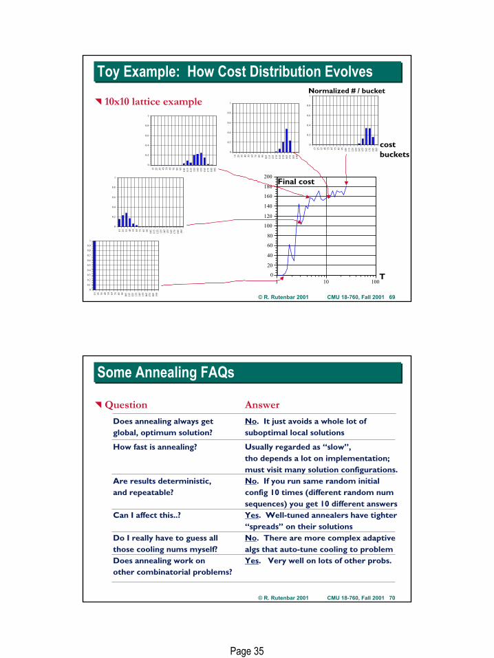
Annealing DynamicsAnnealing Dynamics
What happens to distribution as cooling proceeds?Histograms get narrower: unwilling to visit so many bad configs in the neighborhood, and there are fewer “better” configs around
Histograms get taller: more of the solutions you find are near the mean, temp is too low to jump uphill to really worse ones, and again there are fewer better ones around to fall down into
Count =# observed
configswithin
cost range T = hotter,mean is higherspread is wider
T = colder,mean is lower
spread is narrower
Cost ranges of visited configs
cooling
Page 35
© R. Rutenbar 2001 CMU 18-760, Fall 2001 69
Toy Example: How Cost Distribution EvolvesToy Example: How Cost Distribution Evolves
10x10 lattice example
15 25 35 45 55 65 75 85 95105
115
125
135
145
155
165
175
185
195
0
0.2
0.4
0.6
0.8
1
15 25 35 45 55 65 75 85 95105
115
125
135
145
155
165
175
185
195
0
0.2
0.4
0.6
0.8
1
15 25 35 45 55 65 75 85 95105
115
125
135
145
155
165
175
185
195
0
0.2
0.4
0.6
0.8
115 25 35 45 55 65 75 85 95105
115
125
135
145
155
165
175
185
195
0
0.2
0.4
0.6
0.8
1
15 25 35 45 55 65 75 85 95105
115
125
135
145
155
165
175
185
195
0
0.1
0.2
0.3
0.4
0.5
0.6
0.7
0.8
0.9
1
0
20
40
60
80
100
120
140
160
180
200
1 10 100
Final cost
T
Normalized # / bucket
costbuckets
© R. Rutenbar 2001 CMU 18-760, Fall 2001 70
Some Annealing FAQsSome Annealing FAQs
Question Answer
Does annealing always get No. It just avoids a whole lot ofglobal, optimum solution? suboptimal local solutions
How fast is annealing? Usually regarded as “slow”,tho depends a lot on implementation;must visit many solution configurations.
Are results deterministic, No. If you run same random initialand repeatable? config 10 times (different random num
sequences) you get 10 different answersCan I affect this..? Yes. Well-tuned annealers have tighter
“spreads” on their solutionsDo I really have to guess all No. There are more complex adaptivethose cooling nums myself? algs that auto-tune cooling to problemDoes annealing work on Yes. Very well on lots of other probs. other combinatorial problems?
Page 36
© R. Rutenbar 2001 CMU 18-760, Fall 2001 71
SummarySummary
Annealing isA way of constructing algorithms for combinatorial optimiz. problems
Iterative improvement with hill climbing
Composed of a few essential pieces
State representation, cost function, move set, cooling schedule
Good at not getting stuck in some local minima
ASIC placement3 big strategies: recursive, direct, iterative improvement
2 big optimization goals: estimated total wirelength, congestion
Annealing has been very successful in itetrative improvement placement with total wirelength minimization as the goal
Annealing runs out of gas around 100k-gates
Part II covers recursive & direct techniques (surprise: they are related)