1

Introduction to Electronic Design Automation

Jie-Hong Roland Jiang江介宏

Department of Electrical EngineeringNational Taiwan University

Spring 2014

2

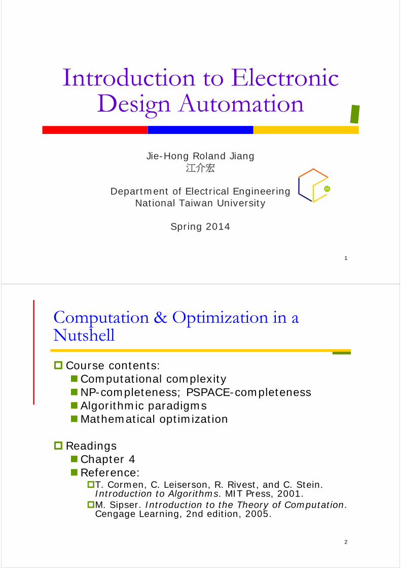
Computation & Optimization in a Nutshell

Course contents:Computational complexityNP-completeness; PSPACE-completenessAlgorithmic paradigmsMathematical optimization

ReadingsChapter 4 Reference:

T. Cormen, C. Leiserson, R. Rivest, and C. Stein. Introduction to Algorithms. MIT Press, 2001.

M. Sipser. Introduction to the Theory of Computation. Cengage Learning, 2nd edition, 2005.

3

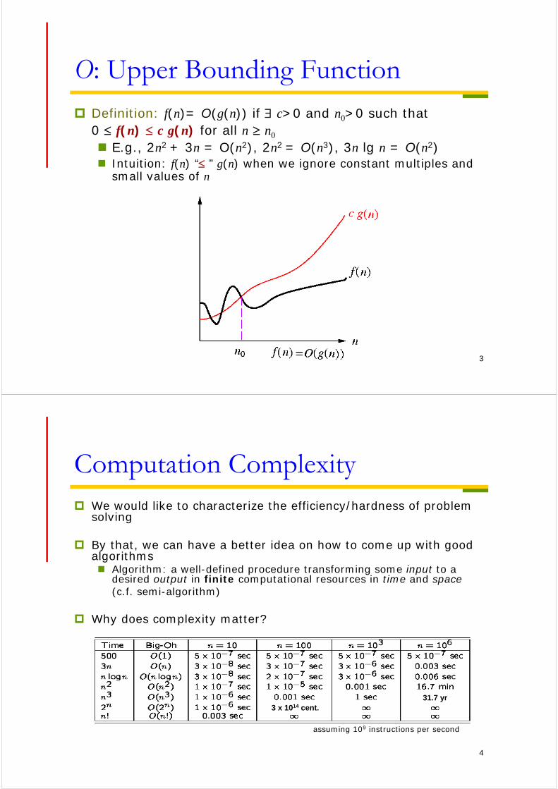
O: Upper Bounding Function Definition: f(n)= O(g(n)) if c>0 and n0>0 such that

0 f(n) c g(n) for all n n0

E.g., 2n2 + 3n = O(n2), 2n2 = O(n3), 3n lg n = O(n2) Intuition: f(n) “ ” g(n) when we ignore constant multiples and

small values of n

4

Computation Complexity We would like to characterize the efficiency/hardness of problem

solving

By that, we can have a better idea on how to come up with good algorithms Algorithm: a well-defined procedure transforming some input to a

desired output in finite computational resources in time and space (c.f. semi-algorithm)

Why does complexity matter?

assuming 109 instructions per second

31.7 yr3 x 1014 cent.

5

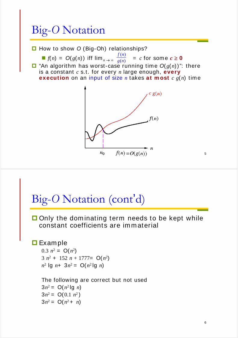
Big-O Notation How to show O (Big-Oh) relationships?

f(n) = O(g(n)) iff limn = c for some c 0 “An algorithm has worst-case running time O(g(n))”: there

is a constant c s.t. for every n large enough, every execution on an input of size n takes at most c g(n) time

( )

( )

f n

g n

6

Big-O Notation (cont’d)

Only the dominating term needs to be kept while constant coefficients are immaterial

Example0.3 n2 = O(n2)3 n2 + 152 n + 1777= O(n2)n2 lg n+ 3n2 = O(n2 lg n)

The following are correct but not used3n2 = O(n2 lg n)3n2 = O(0.1 n2 )3n2 = O(n2 + n)

7

Other Asymptotic BoundsOther notations (though not important for now): Definition: f(n)= (g(n)) if c, n0 > 0 such that

0 c g(n) f(n) for all n n0. -notation provides an asymptotic lower bound on a function

Definition: f(n)= (g(n)) if c1, c2, n0 > 0 such that 0 c1 g(n) f(n) c2 g(n) for all n n0.

-notation provides an asymptotic tight bound on a function

Showing the complexity upper bound of solving a problem (not an instance) is often much easier than showing the complexity lower bound Why?

8

Computational Complexity

Computational complexity: an abstract measure of the time and space necessary to execute an algorithm as function of its “input size”

Input size examples: sort n words of bounded length n the input is the integer n lg n the input is the graph G(V, E) |V| and |E|

Time complexity is expressed in elementary computational steps (e.g., an addition, multiplication, pointer indirection)

Space complexity is expressed in memory locations (e.g. bits, bytes, words)

9

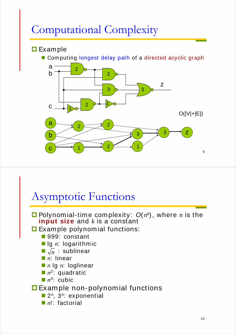
Computational Complexity

Example Computing longest delay path of a directed acyclic graph

ab

z

c 11

2

2

2

3 3

a

b

c

z2

2

2

3 3

1 1

O(|V|+|E|)

10

Asymptotic Functions

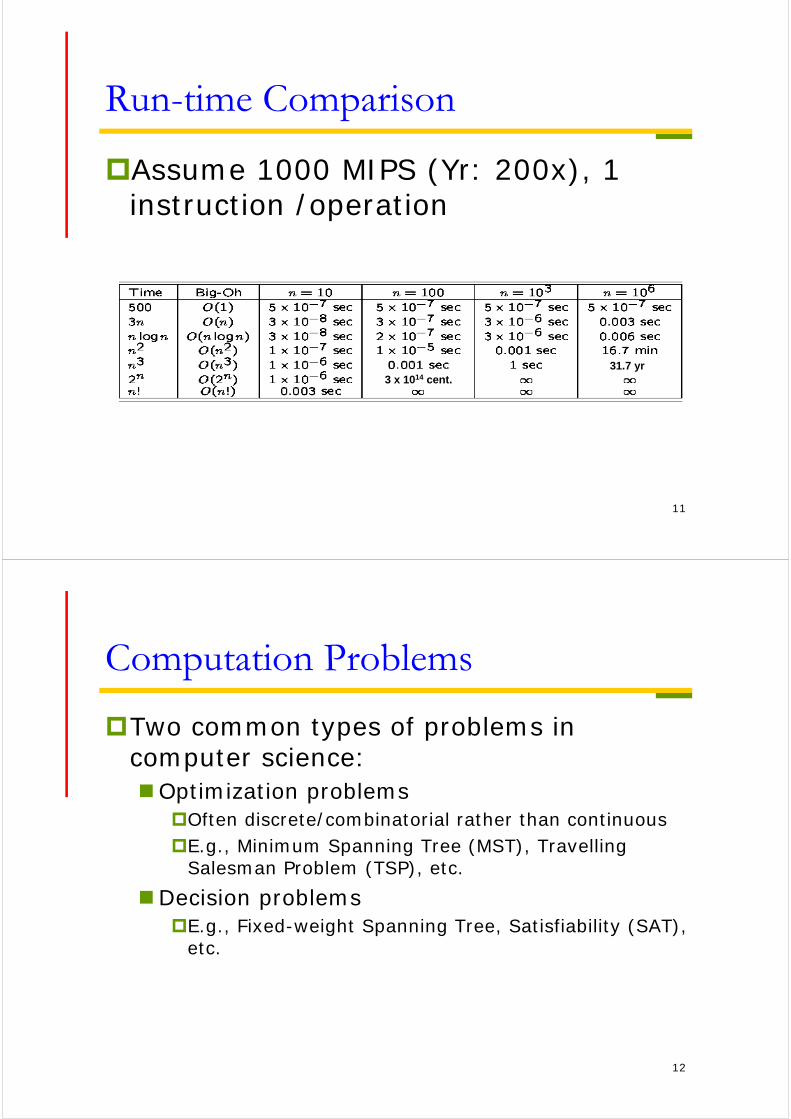
Polynomial-time complexity: O(nk), where n is the input size and k is a constant

Example polynomial functions: 999: constant lg n: logarithmic : sublinear n: linear n lg n: loglinear n2: quadratic n3: cubic

Example non-polynomial functions 2n, 3n: exponential n!: factorial

n

11

Run-time Comparison

Assume 1000 MIPS (Yr: 200x), 1 instruction /operation

31.7 yr3 x 1014 cent.

12

Computation Problems

Two common types of problems in computer science:Optimization problems

Often discrete/combinatorial rather than continuousE.g., Minimum Spanning Tree (MST), Travelling

Salesman Problem (TSP), etc.

Decision problemsE.g., Fixed-weight Spanning Tree, Satisfiability (SAT),

etc.

13

Terminology Problem: a general class, e.g., “the shortest-path problem for

directed acyclic graphs” Instance: a specific case of a problem, e.g., “the shortest-

path problem in a specific graph, between two given vertices” Optimization problems: those finding a legal configuration

such that its cost is minimum (or maximum) MST: Given a graph G=(V, E), find the cost of a minimum

spanning tree of G An instance I = (F, c) where

F is the set of feasible solutions, and c is a cost function, assigning a cost value to each feasible

solution c : F R The solution of the optimization problem is the feasible

solution with optimal (minimal/maximal) cost c.f., optimal solutions/costs, optimal (exact) algorithms (Attn:

optimal exact in the theoretic computer science community)

14

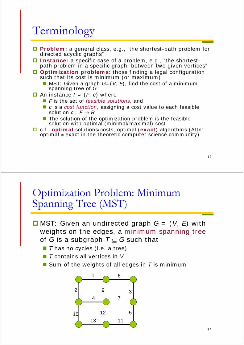
Optimization Problem: Minimum Spanning Tree (MST)

MST: Given an undirected graph G = (V, E) with weights on the edges, a minimum spanning tree of G is a subgraph T G such that T has no cycles (i.e. a tree) T contains all vertices in V Sum of the weights of all edges in T is minimum

1 6

2

10

4

13

7

11

9

12

3

5

15

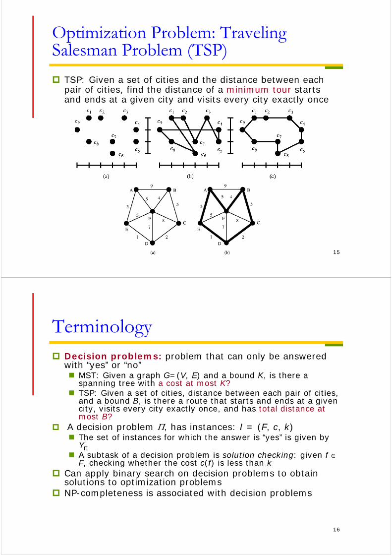
Optimization Problem: Traveling Salesman Problem (TSP)

TSP: Given a set of cities and the distance between each pair of cities, find the distance of a minimum tour starts and ends at a given city and visits every city exactly once

16

Terminology Decision problems: problem that can only be answered

with “yes” or “no” MST: Given a graph G=(V, E) and a bound K, is there a

spanning tree with a cost at most K? TSP: Given a set of cities, distance between each pair of cities,

and a bound B, is there a route that starts and ends at a given city, visits every city exactly once, and has total distance at most B?

A decision problem , has instances: I = (F, c, k) The set of instances for which the answer is “yes” is given by

Y A subtask of a decision problem is solution checking: given f

F, checking whether the cost c(f) is less than k Can apply binary search on decision problems to obtain

solutions to optimization problems NP-completeness is associated with decision problems

17

Decision Problem: Fixed-weight Spanning Tree

Given an undirected graph G = (V, E), is there a spanning tree of G with weight c?

Can solve MST by posing it as a sequence of decision problems (with binary search)

18

Decision Problem: SatisfiabilityProblem (SAT)

Satisfiability Problem (SAT): Instance: A Boolean formula in conjunctive normal

form (CNF), a.k.a. product-of-sums (POS) Question: Is there an assignment of Boolean values to

the variables that makes true ?

A Boolean formula is satisfiable if there exists a a set of Boolean input values that makes valuate to true. Otherwise, is unsatisfiable. (a+b)(a+c)(b+c) is satisfiable since (a, b, c) = (0, 1,

0) makes the formula true. (a+b)(a+c)(b)(c) is unsatisfiable

19

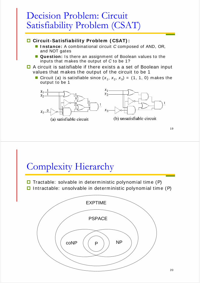
Decision Problem: Circuit Satisfiability Problem (CSAT)

Circuit-Satisfiability Problem (CSAT): Instance: A combinational circuit C composed of AND, OR,

and NOT gates Question: Is there an assignment of Boolean values to the

inputs that makes the output of C to be 1? A circuit is satisfiable if there exists a a set of Boolean input

values that makes the output of the circuit to be 1 Circuit (a) is satisfiable since (x1, x2, x3) = (1, 1, 0) makes the

output to be 1

20

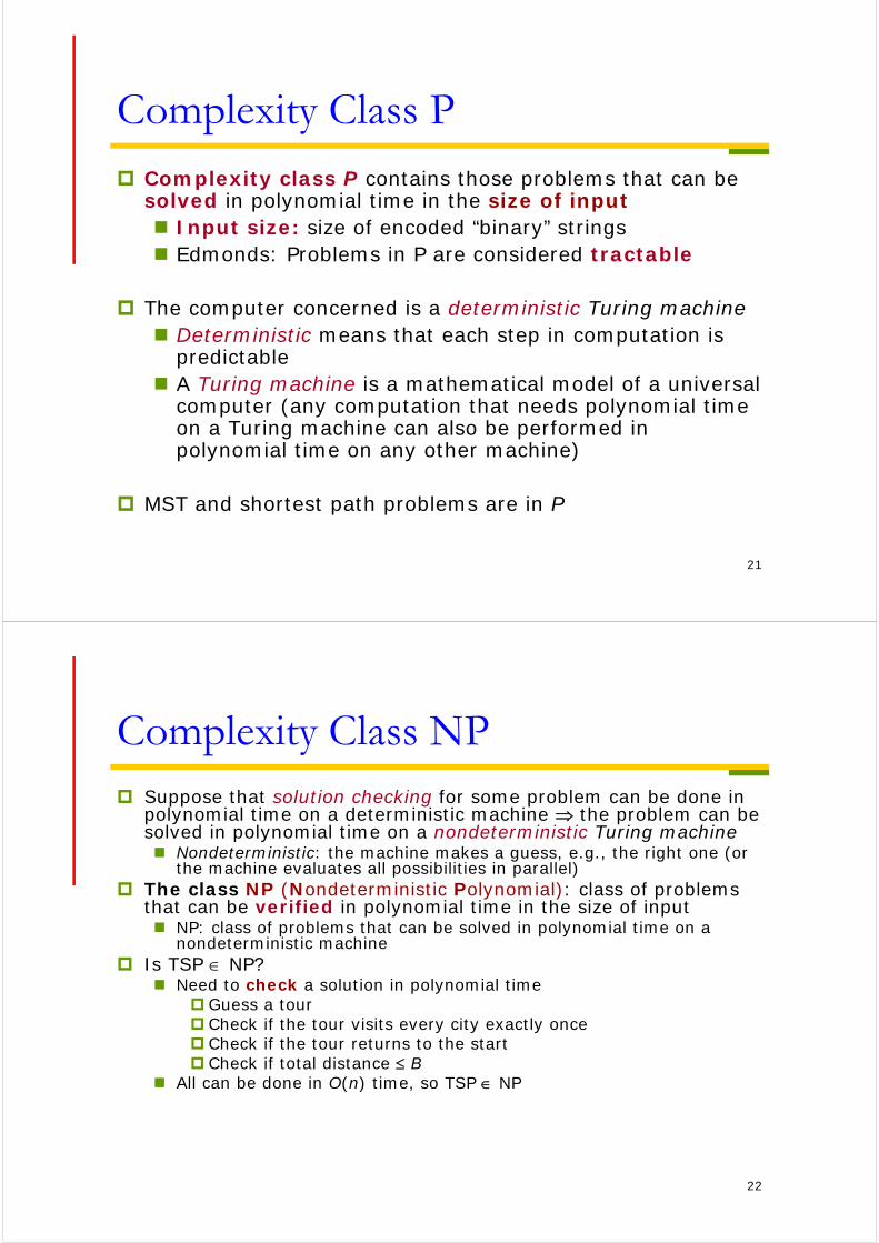
Complexity Hierarchy Tractable: solvable in deterministic polynomial time (P) Intractable: unsolvable in deterministic polynomial time (P)

PcoNP NP

PSPACE

EXPTIME

21

Complexity Class P Complexity class P contains those problems that can be

solved in polynomial time in the size of input Input size: size of encoded “binary” strings Edmonds: Problems in P are considered tractable

The computer concerned is a deterministic Turing machine Deterministic means that each step in computation is

predictable A Turing machine is a mathematical model of a universal

computer (any computation that needs polynomial time on a Turing machine can also be performed in polynomial time on any other machine)

MST and shortest path problems are in P

22

Complexity Class NP Suppose that solution checking for some problem can be done in

polynomial time on a deterministic machine the problem can be solved in polynomial time on a nondeterministic Turing machine Nondeterministic: the machine makes a guess, e.g., the right one (or

the machine evaluates all possibilities in parallel) The class NP (Nondeterministic Polynomial): class of problems

that can be verified in polynomial time in the size of input NP: class of problems that can be solved in polynomial time on a

nondeterministic machine Is TSP NP?

Need to check a solution in polynomial time Guess a tour Check if the tour visits every city exactly once Check if the tour returns to the start Check if total distance B

All can be done in O(n) time, so TSP NP

23

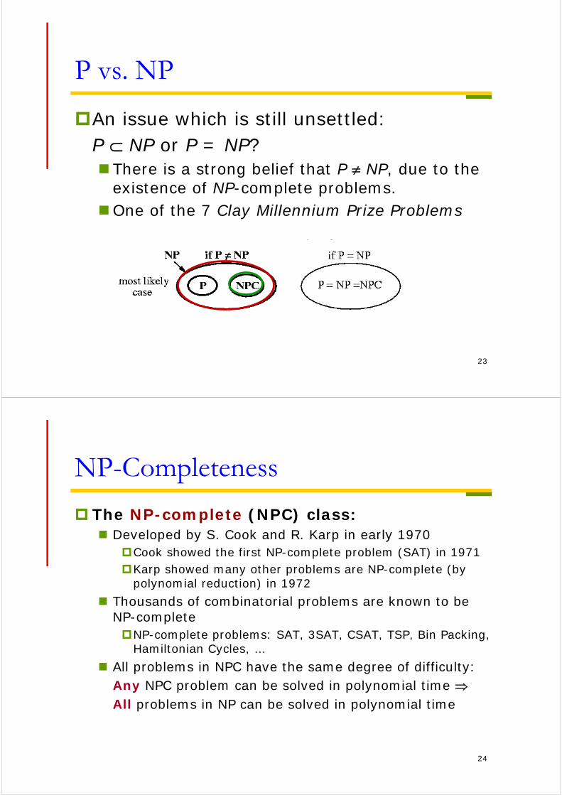
P vs. NP

An issue which is still unsettled:P NP or P = NP? There is a strong belief that P NP, due to the

existence of NP-complete problems.One of the 7 Clay Millennium Prize Problems

24

NP-Completeness

The NP-complete (NPC) class: Developed by S. Cook and R. Karp in early 1970

Cook showed the first NP-complete problem (SAT) in 1971Karp showed many other problems are NP-complete (by

polynomial reduction) in 1972

Thousands of combinatorial problems are known to be NP-completeNP-complete problems: SAT, 3SAT, CSAT, TSP, Bin Packing,

Hamiltonian Cycles, …

All problems in NPC have the same degree of difficulty: Any NPC problem can be solved in polynomial time All problems in NP can be solved in polynomial time

25

Beyond NP

A quantified Boolean formula (QBF) is Q1 x1, Q2 x2, …, Qn xn. where Qi is either a existential () or universal quantifier (), xi is a Boolean variable, and is a Boolean formula i: X1,X2,X3, …,QnXi. i: X1,X2,X3, …,QnXi.

Xi is a variable set (XiXj = for i j)

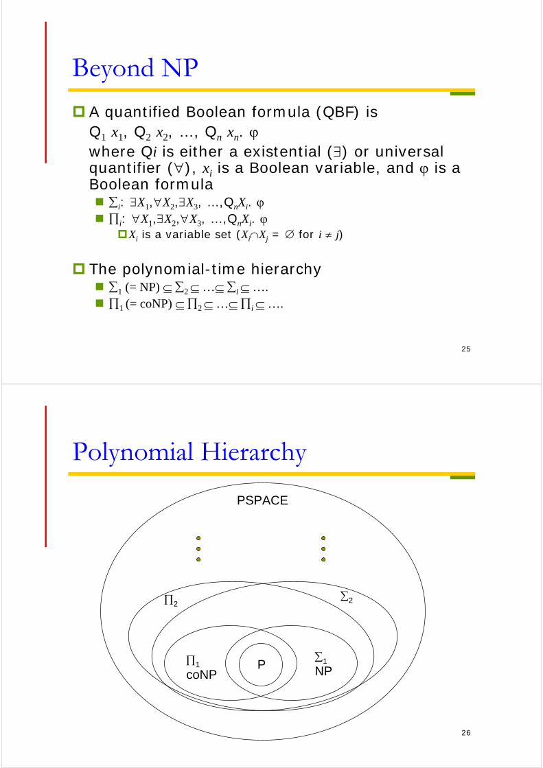
The polynomial-time hierarchy 1 (= NP) 2 … i …. 1 (= coNP) 2 … i ….

26

Polynomial Hierarchy

P1

coNP

1

NP

PSPACE

22

27

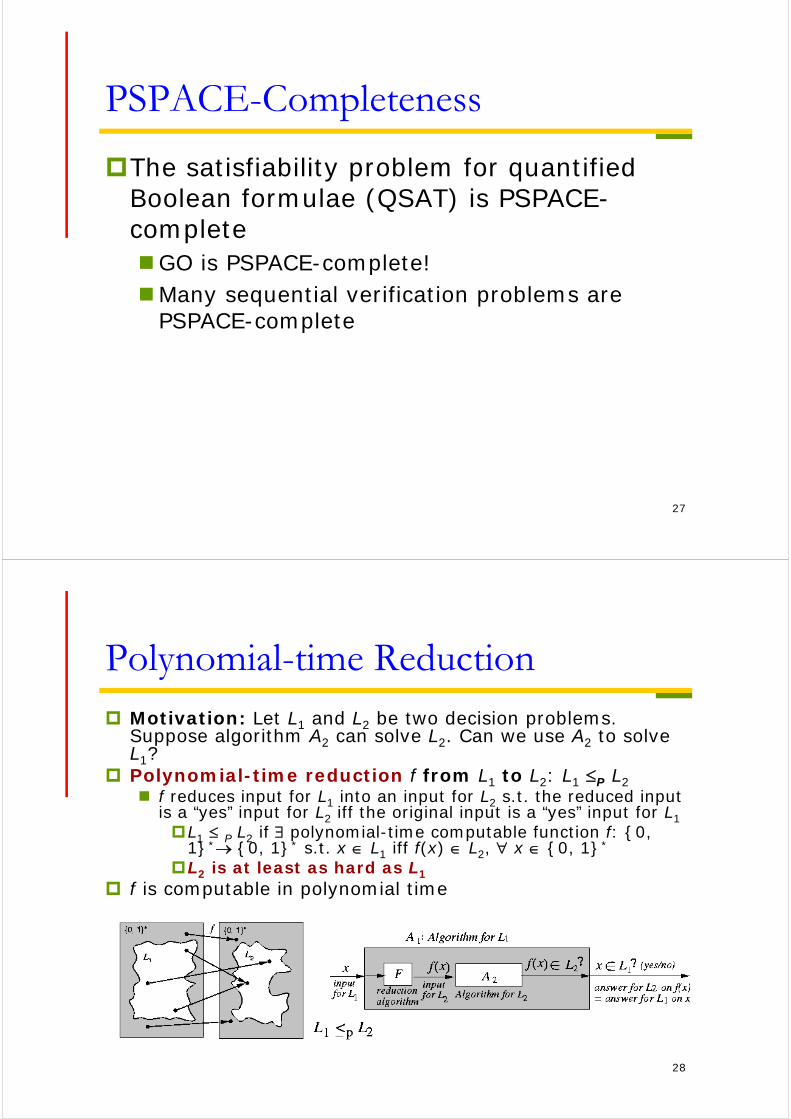
PSPACE-Completeness

The satisfiability problem for quantified Boolean formulae (QSAT) is PSPACE-completeGO is PSPACE-complete!Many sequential verification problems are

PSPACE-complete

28

Polynomial-time Reduction Motivation: Let L1 and L2 be two decision problems.

Suppose algorithm A2 can solve L2. Can we use A2 to solve L1?

Polynomial-time reduction f from L1 to L2: L1 P L2 f reduces input for L1 into an input for L2 s.t. the reduced input

is a “yes” input for L2 iff the original input is a “yes” input for L1L1 P L2 if polynomial-time computable function f: {0,

1}* {0, 1}* s.t. x L1 iff f(x) L2, x {0, 1}*

L2 is at least as hard as L1

f is computable in polynomial time

29

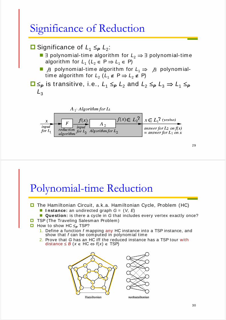
Significance of Reduction

Significance of L1 P L2: polynomial-time algorithm for L2 polynomial-time

algorithm for L1 (L2 P L1 P) polynomial-time algorithm for L1 polynomial-

time algorithm for L2 (L1 P L2 P)

P is transitive, i.e., L1 P L2 and L2 P L3 L1 PL3

30

Polynomial-time Reduction The Hamiltonian Circuit, a.k.a. Hamiltonian Cycle, Problem (HC)

Instance: an undirected graph G = (V, E) Question: is there a cycle in G that includes every vertex exactly once?

TSP (The Traveling Salesman Problem) How to show HC P TSP?

1. Define a function f mapping any HC instance into a TSP instance, and show that f can be computed in polynomial time

2. Prove that G has an HC iff the reduced instance has a TSP tour with distance B (x HC f(x) TSP)

31

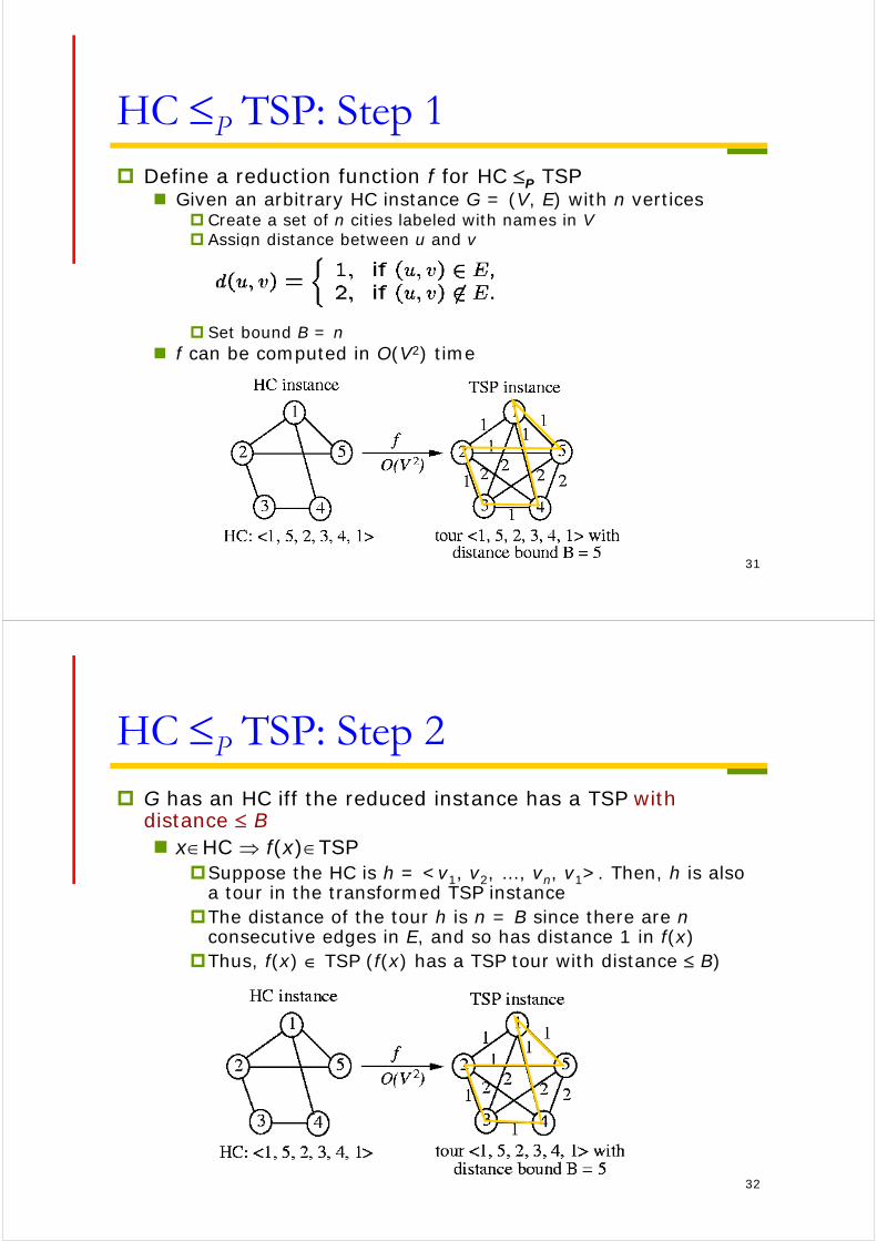
HC P TSP: Step 1 Define a reduction function f for HC P TSP

Given an arbitrary HC instance G = (V, E) with n vertices Create a set of n cities labeled with names in V Assign distance between u and v

Set bound B = n f can be computed in O(V2) time

32

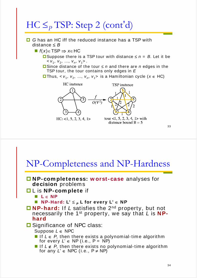
HC P TSP: Step 2 G has an HC iff the reduced instance has a TSP with

distance B xHC f(x)TSP

Suppose the HC is h = <v1, v2, …, vn, v1>. Then, h is also a tour in the transformed TSP instance

The distance of the tour h is n = B since there are nconsecutive edges in E, and so has distance 1 in f(x)

Thus, f(x) TSP (f(x) has a TSP tour with distance B)

33

HC P TSP: Step 2 (cont’d) G has an HC iff the reduced instance has a TSP with

distance B f(x)TSP xHC

Suppose there is a TSP tour with distance n = B. Let it be <v1, v2, …, vn, v1>.

Since distance of the tour n and there are n edges in the TSP tour, the tour contains only edges in E

Thus, <v1, v2, …, vn, v1> is a Hamiltonian cycle (x HC)

34

NP-Completeness and NP-Hardness

NP-completeness: worst-case analyses for decision problems

L is NP-complete if L NP NP-Hard: L' P L for every L' NP

NP-hard: If L satisfies the 2nd property, but not necessarily the 1st property, we say that L is NP-hard

Significance of NPC class:Suppose L NPC If L P, then there exists a polynomial-time algorithm

for every L' NP (i.e., P = NP) If L P, then there exists no polynomial-time algorithm

for any L' NPC (i.e., P NP)

35

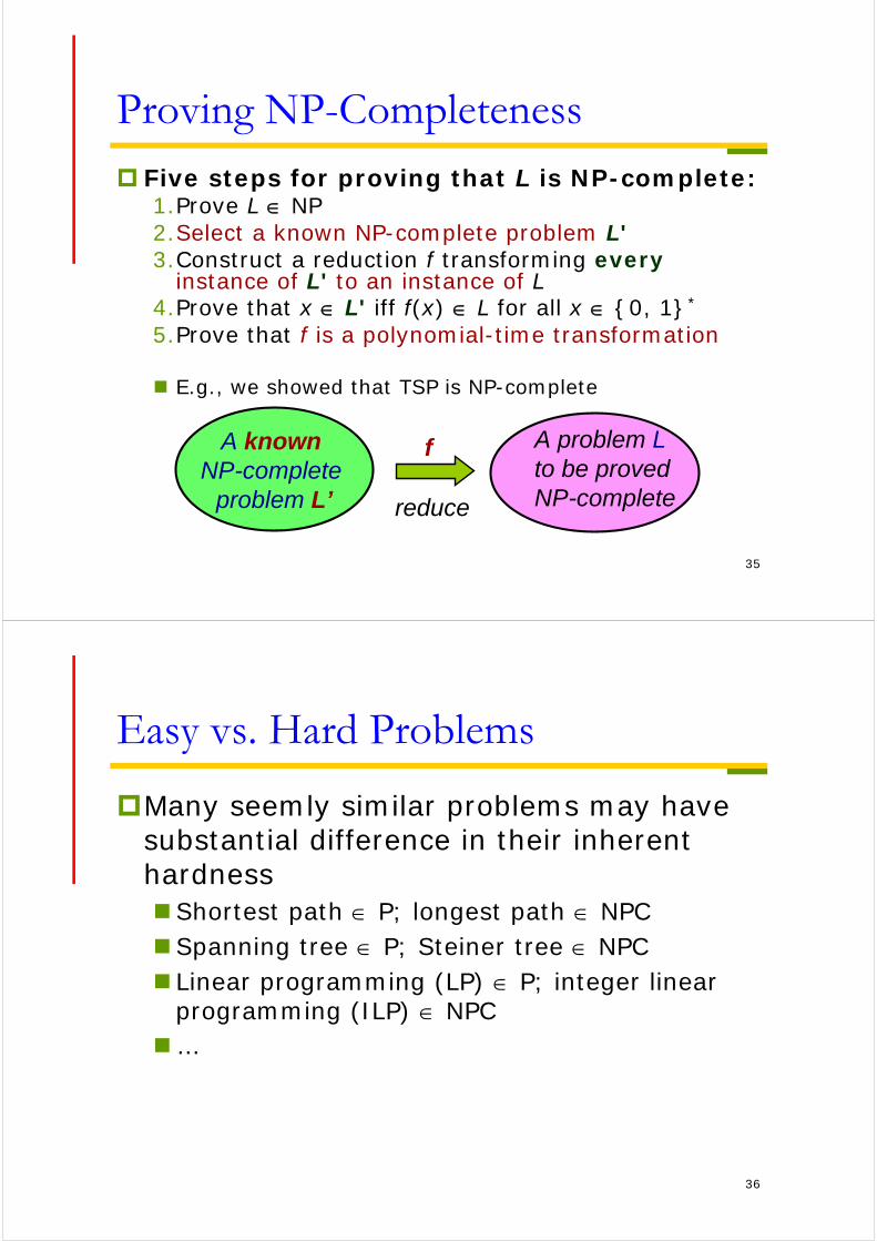
Proving NP-Completeness

Five steps for proving that L is NP-complete:1.Prove L NP2.Select a known NP-complete problem L'3.Construct a reduction f transforming every

instance of L' to an instance of L4.Prove that x L' iff f(x) L for all x {0, 1}*

5.Prove that f is a polynomial-time transformation

E.g., we showed that TSP is NP-complete

A knownNP-complete

problem L’

A problem Lto be proved NP-completereduce

f

36

Easy vs. Hard Problems

Many seemly similar problems may have substantial difference in their inherent hardnessShortest path P; longest path NPCSpanning tree P; Steiner tree NPC Linear programming (LP) P; integer linear

programming (ILP) NPC…

37

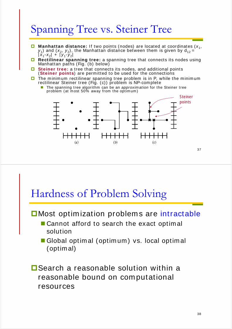
Spanning Tree vs. Steiner Tree Manhattan distance: If two points (nodes) are located at coordinates (x1,

y1) and (x2, y2), the Manhattan distance between them is given by d12 = |x1-x2| + |y1-y2|

Rectilinear spanning tree: a spanning tree that connects its nodes using Manhattan paths (Fig. (b) below)

Steiner tree: a tree that connects its nodes, and additional points (Steiner points) are permitted to be used for the connections

The minimum rectilinear spanning tree problem is in P, while the minimum rectilinear Steiner tree (Fig. (c)) problem is NP-complete The spanning tree algorithm can be an approximation for the Steiner tree

problem (at most 50% away from the optimum)

Steiner points

38

Hardness of Problem Solving

Most optimization problems are intractableCannot afford to search the exact optimal

solutionGlobal optimal (optimum) vs. local optimal

(optimal)

Search a reasonable solution within a reasonable bound on computational resources

39

Coping with NP-hard Problems Approximation algorithms

Guarantee to be a fixed percentage away from the optimum E.g., MST for the minimum Steiner tree problem

Randomized algorithms Trade determinism for efficiency

Pseudo-polynomial time algorithms Has the form of a polynomial function for the complexity, but is not to

the problem size E.g., O(nW) for the 0-1 knapsack problem

Restriction Work on some subset of the original problem E.g., longest path problem restricted to directed acyclic graphs

Exhaustive search/Branch and bound Is feasible only when the problem size is small

Local search: Simulated annealing (hill climbing), genetic algorithms, etc.

Heuristics: No guarantee of performance

40

Algorithmic Paradigms Exhaustive search: Search the entire solution space Branch and bound: A search technique with pruning Greedy method: Pick a locally optimal solution at each step Dynamic programming: Partition a problem into a collection of

sub-problems, the sub-problems are solved, and then the original problem is solved by combining the solutions (applicable when the sub-problems are NOT independent)

Hierarchical approach: Divide-and-conquer Mathematical programming: A system of solving an objective

function under constraints Simulated annealing: An adaptive, iterative, non-deterministic

algorithm that allows “uphill” moves to escape from local optima Tabu search: Similar to simulated annealing, but does not

decrease the chance of “uphill” moves throughout the search Genetic algorithm: A population of solutions is stored and

allowed to evolve through successive generations via mutation, crossover, etc.

41

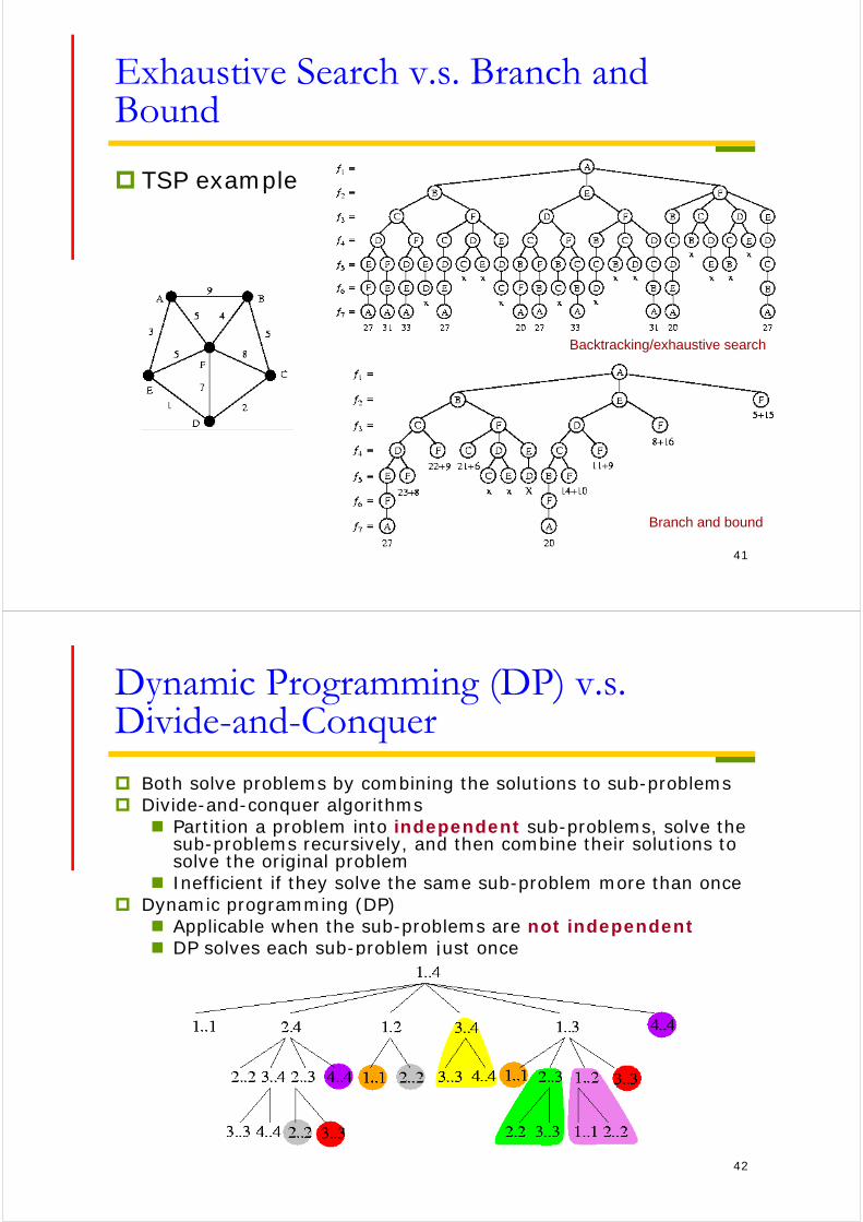
Exhaustive Search v.s. Branch and Bound

TSP example

Backtracking/exhaustive search

Branch and bound

42

Dynamic Programming (DP) v.s. Divide-and-Conquer

Both solve problems by combining the solutions to sub-problems Divide-and-conquer algorithms

Partition a problem into independent sub-problems, solve the sub-problems recursively, and then combine their solutions to solve the original problem

Inefficient if they solve the same sub-problem more than once Dynamic programming (DP)

Applicable when the sub-problems are not independent DP solves each sub-problem just once

43

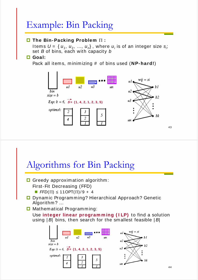
Example: Bin Packing The Bin-Packing Problem :

Items U = {u1, u2, …, un}, where ui is of an integer size si; set B of bins, each with capacity b

Goal:Pack all items, minimizing # of bins used (NP-hard!)

S = (1, 4, 2, 1, 2, 3, 5)

44

Algorithms for Bin Packing Greedy approximation algorithm:

First-Fit Decreasing (FFD) FFD() 11OPT()/9 + 4

Dynamic Programming? Hierarchical Approach? Genetic Algorithm? …

Mathematical Programming: Use integer linear programming (ILP) to find a solution using |B| bins, then search for the smallest feasible |B|

S = (1, 4, 2, 1, 2, 3, 5)

45

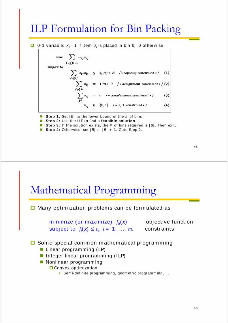
ILP Formulation for Bin Packing 0-1 variable: xij=1 if item ui is placed in bin bj, 0 otherwise

Step 1: Set |B| to the lower bound of the # of bins Step 2: Use the ILP to find a feasible solution Step 3: If the solution exists, the # of bins required is |B|. Then exit. Step 4: Otherwise, set |B| |B| + 1. Goto Step 2.

46

Mathematical Programming Many optimization problems can be formulated as

minimize (or maximize) f0(x) objective functionsubject to fi(x) ci, i = 1, …, m. constraints

Some special common mathematical programming Linear programming (LP) Integer linear programming (ILP) Nonlinear programming

Convex optimization Semi-definite programming, geometric programming, …