Embed Size (px)
Citation preview
Gradient descent methods•Choosing the descent direction•Choosing the step size•Convergence•Convergence rate•
This lecture:
Instructor: Amir Ali Ahmadi
Fall 2014
Learned about some structural properties of local optimal solutions (first and second order conditions for optimality).
•
Learned that for convex problems, local optima are automatically global.•But how to find a local optimum?•How to even find a stationary point (i.e., a point where the gradient vanishes)? Recall that this would suffice for global optimality if is convex.
•
We now begin to see some algorithms for this purpose, starting with gradient descent algorithms.
•
These will be iterative algorithms: start at a point, jump to a new point that hopefully has a lower objective value and continue.
•
Our presentation uses references [Bert03], [Bert09], [Tit13], [CZ13].•
Where we stand so far:
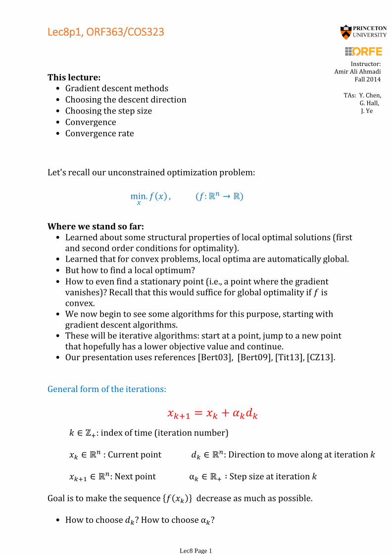
Let's recall our unconstrained optimization problem:
index of time (iteration number)
: Current point
Next point
: Direction to move along at iteration
Step size at iteration
General form of the iterations:
How to choose ? How to choose ?•
Goal is to make the sequence decrease as much as possible.
TAs: Y. Chen, G. Hall, J. Ye
Lec8p1, ORF363/COS323
Lec8 Page 1
Gradient methods
Throughout this lecture, we assume that is at least (continuously differentiable).
•
Gradient methods: the direction to move along at step is chosen "based on information from"
•
Why is a natural vector to look at? Lemmas 1 and 2 below (proved on the next page) provide two reasons.
•
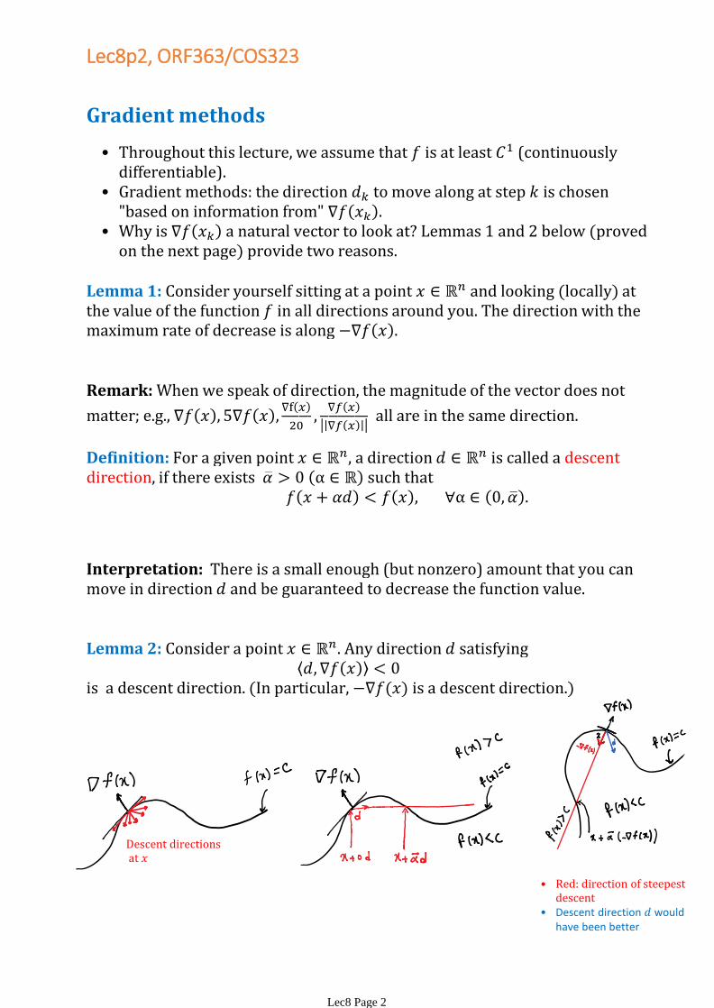
Lemma 1: Consider yourself sitting at a point and looking (locally) at the value of the function in all directions around you. The direction with the maximum rate of decrease is along
Lemma 2: Consider a point . Any direction satisfying is a descent direction. (In particular, is a descent direction.)
Definition: For a given point a direction is called a descent direction, if there exists such that
Remark: When we speak of direction, the magnitude of the vector does not
matter; e.g.,
all are in the same direction.
Interpretation: There is a small enough (but nonzero) amount that you can move in direction and be guaranteed to decrease the function value.
Descent directionsat
Red: direction of steepest descent
•
Descent direction would have been better
•
Lec8p2, ORF363/COS323
Lec8 Page 2

Remark: The condition in Lemma 2 geometrically means that the vectors and make an angle of more than 90 degrees (on the plane that contains them).
Why?
Proof of Lemma 1.Consider a point , a direction , and the univariate function
The rate of change of at in direction is given by which by the chain rule equals
By the Cauchy-Schwarz inequality (see, e.g., Theorem 2.3 of [CZ13] for a proof), we have:
which after simplifying gives
So the rate of change in any direction cannot be larger than or
smaller than However, if we take the right inequality is achieved:
Proof of Lemma 2.
By Taylor's theorem, we have
Since
there exists such that
).
This, together with our assumption that implies that ) we must have: Hence, is a descent direction.
Similarly, if we take then the left inequality is achieved.
Lec8p3, ORF363/COS323
Lec8 Page 3
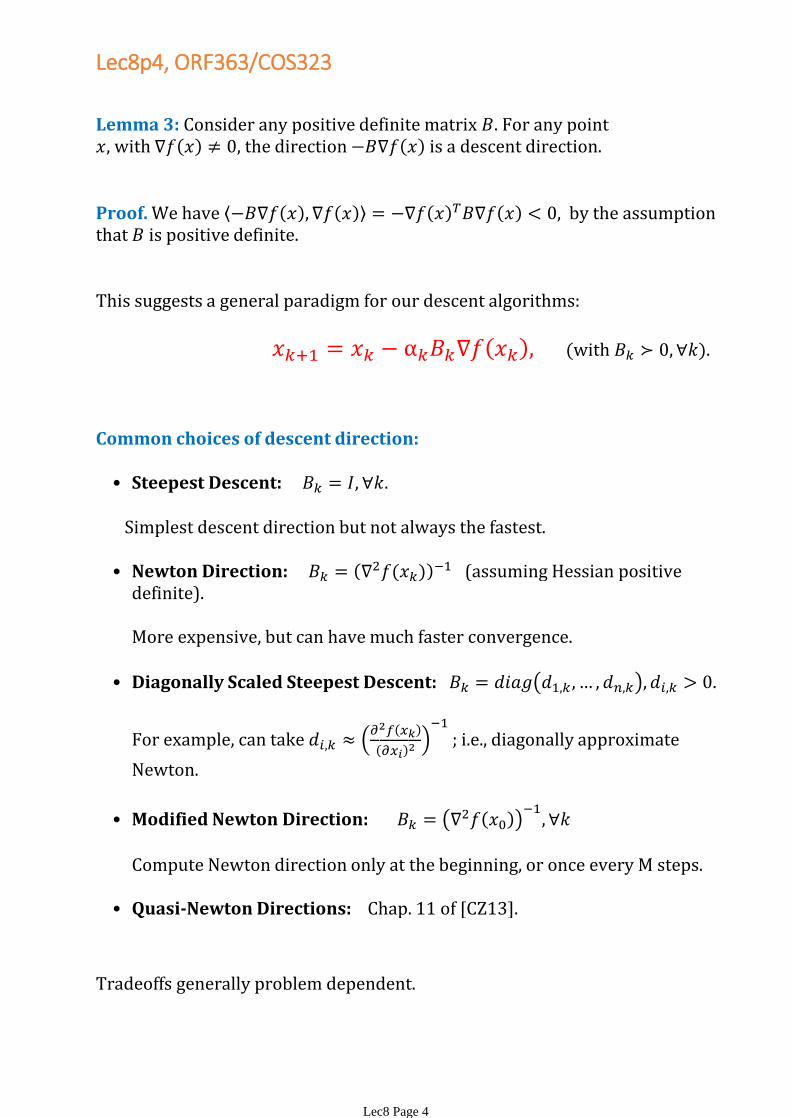
Lemma 3: Consider any positive definite matrix . For any point with , the direction is a descent direction.
Proof. We have by the assumption that is positive definite.
This suggests a general paradigm for our descent algorithms:
(with ).
Common choices of descent direction:
Steepest Descent: •
Simplest descent direction but not always the fastest.
Newton Direction: (assuming Hessian positive
definite).
More expensive, but can have much faster convergence.
•
Diagonally Scaled Steepest Descent:
For example, can take
i.e., diagonally approximate
Newton.
•
Modified Newton Direction:
•
Compute Newton direction only at the beginning, or once every M steps.
Quasi-Newton Directions: Chap. 11 of [CZ13].•
Tradeoffs generally problem dependent.
Lec8p4, ORF363/COS323
Lec8 Page 4

Common choices of the step size
Back to the general form of our iterative algorithm:
Constant step size: •
Simplest rule to implement, but may not converge if too large; may be too slow if too small.
○
Diminishing step size: (e.g.,
)•
Descent not guaranteed at each step; only later when becomes small.
○
imposed to guarantee progress does not become too
slow.○
Good theoretical guarantees, but unless the right sequence is chosen, can also be a slow method.
○
A minimization problem itself, but an easier one (one dimensional).○
Can use the line search methods that we learned in the previous lecture.
○
No need to be very precise at each step.○
If convex, the one dimensional minimization problem also convex (why?).
○
Minimization rule (exact line search): •
Limited minimization: •
Previous comments apply.○
Tries not to step too far.○
Successive step size reduction: well-known examples are Armijo rule and Goldstein rule (see, e.g., Section 7.8 of [CZ13]). We will cover Armijo in the next lecture.
•
Try to ensure enough decrease in line search without spending time to solve it to optimality.
○
Tradeoffs generally problem dependent.
Lec8p5, ORF363/COS323
Lec8 Page 5

An illustration of a single step of the minimization rule (aka exact line search) for choosing the step size.
Image credit: [CZ13]
Stopping criteria.
Once we have a rule for choosing the search direction and the step size, we are good to go for running the algorithm.
•
Typically the initial point is picked randomly, or if we have a guess for the location of local minima, we pick close to them.
•
But when to stop the algorithm?•
Note: if we have , our iterates stop moving. We have found a point satisfying the first order necessary condition for optimality. This is what we are aiming for.
○
Improvements in function value are saturating.
○
Movement between iterates has become small.
○
A "relative" measure - removes dependence on the scale of
The max is taken to avoid dividing by small numbers.
○
Same comments apply.
○
Some common choices ( >0 is a small prescribed threshold):•
Lec8p6, ORF363/COS323
Lec8 Page 6
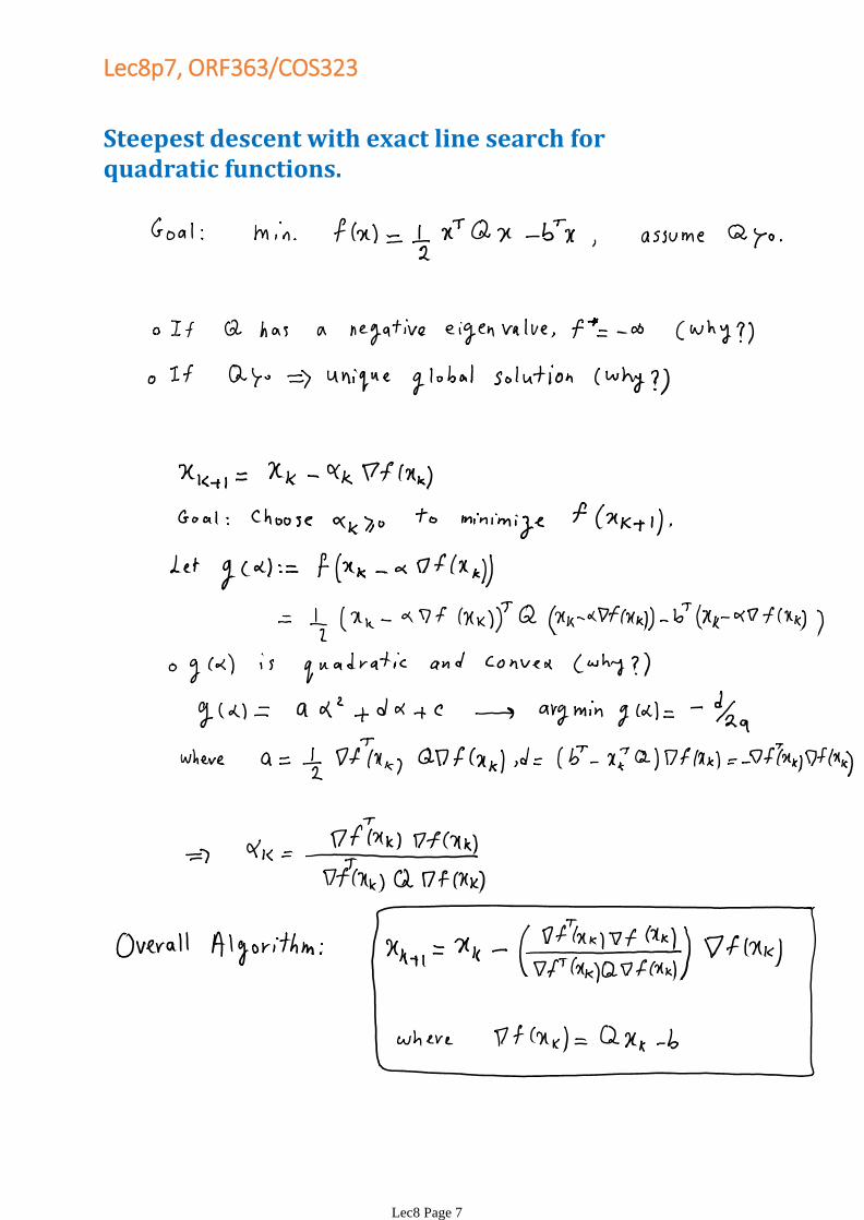
Steepest descent with exact line search for quadratic functions.
Lec8p7, ORF363/COS323
Lec8 Page 7
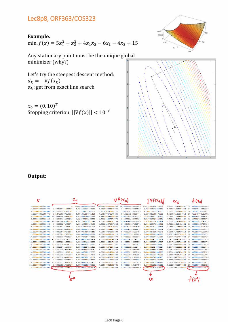
Example.
Any stationary point must be the unique global minimizer (why?)
Let's try the steepest descent method: get from exact line search
Stopping criterion:
Output:
Lec8p8, ORF363/COS323
Lec8 Page 8
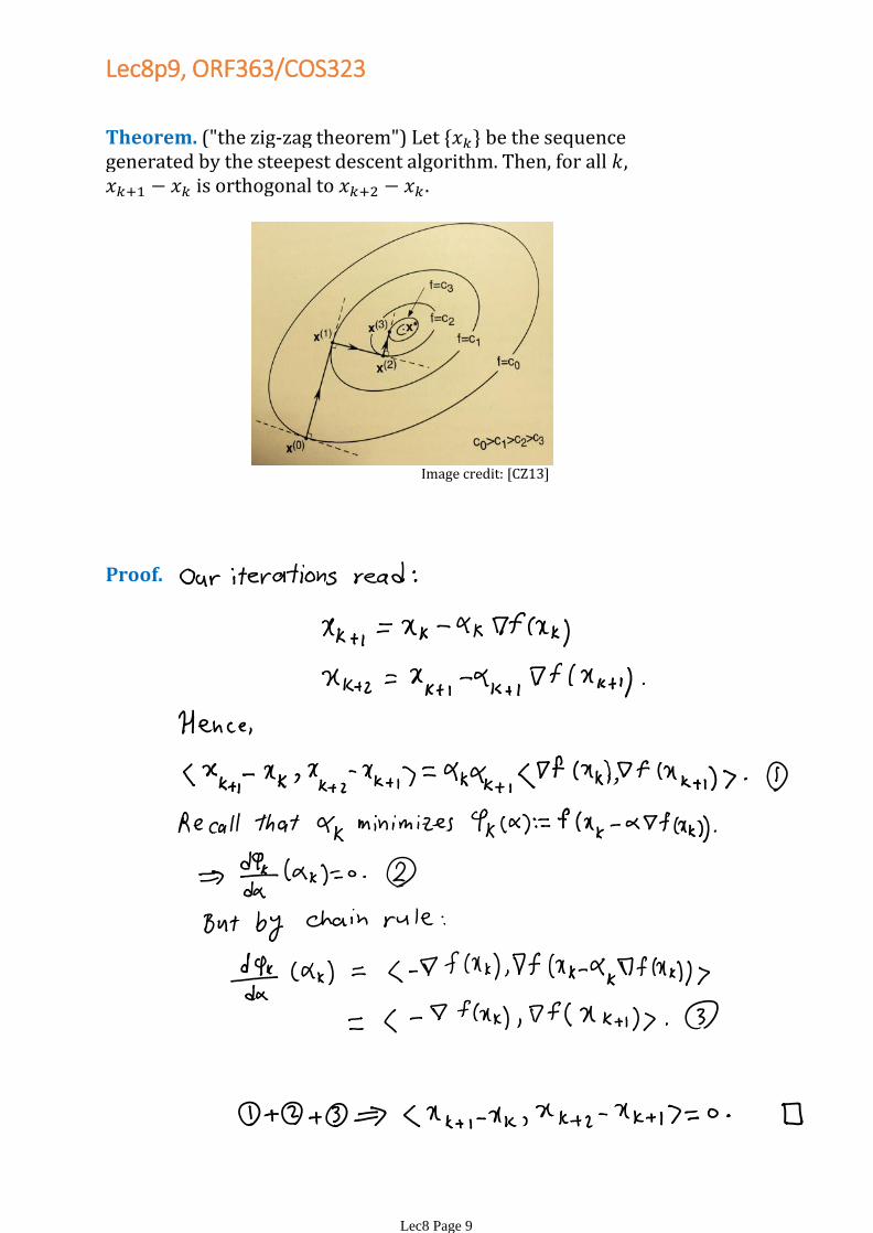
Theorem. ("the zig-zag theorem") Let be the sequence generated by the steepest descent algorithm. Then, for all , is orthogonal to
Proof.
Image credit: [CZ13]
Lec8p9, ORF363/COS323
Lec8 Page 9

Convergence
For the steepest descent algorithm with exact line search, we have starting from any (This is called global convergence.)
•
For the steepest descent algorithm with a fixed step size, we have global convergence if and only if the step size satisfies:
where denotes the maximum eigenvalue of
•
Theorem. (See [CZ13].) Consider a quadratic function
with and let be the
minimizer.
The descent algorithms discussed so far typically come with proofs of convergence to a stationary point. We state a couple such theorems here; the proofs are a bit tedious, and I won't require you to know them. But those interested can look some of these proofs up in [CZ13].
Theorem. (See [Bert03].) Consider the sequence generated by any descent algorithm with such that eigenvalues of are larger than some for all and the step size is chosen according to the minimization rule, or the limited minimization rule, (or the Armijo rule). Then, every limit point of is a stationary point.
Remark1: We say is a limit point of a sequence if there exists a subsequence of that converges to
Remark2: A stationary point may not be a local min! It may be a saddle point or even a local max! But there is a result called the ``capture theorem'' (see [Bert03]) which informally states that isolated local minima tend to attract gradient methods.
Question to think about: How would you check if the point that you end up with (assuming it is stationary) is actually a local minimum?
Lec8p10, ORF363/COS323
Lec8 Page 10
Rates of convergence
Once we know an iterative algorithm converges, the next question is how fast?
•
If
then sure, it will go to zero. But to see the
error go even below 0.1, you need to write a letter to your grandson (to ask for a letter to his grandson, etc.)
•
Let us formalize this.•
Definition (see [Tit13]). Let converge to We say the convergence is of order and with factor if such that
The larger the power the faster the convergence.•For the same the smaller the faster the convergence.•If converges with order , it also converges with order for any
•
If converges with order and factor , it also converges with order and factor for any
•
So we typically look for the largest and the smallest for which the inequality holds.
•
Make sure the following comments make sense:
If and , we say convegence is linear.•If and , we say convegence is sublinear.•If , we say that convergence is superlinear. (This is slightly stronger than the usual definition of superlinear convergence, but we will go with it.)
•
If , we say that convergence is quadratic.•
Some more terminology:
Why called linear convergence?-
For large enough, we have So
Hence, which is a
measure of the number of correct significant digits in grows linearly with
Lec8p11, ORF363/COS323
Lec8 Page 11
Examples:
sublinear convergence.•
linear convergence.•
quadratic convergence.•
(Verify!)
Quadratic convergence is super fast! Number of correct significant digit doubles in each iteration (why?).
•
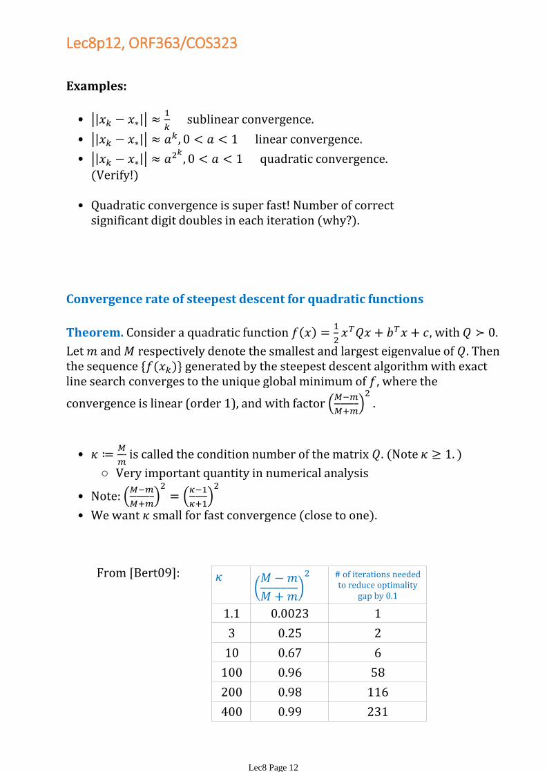
Convergence rate of steepest descent for quadratic functions
Theorem. Consider a quadratic function
with
Let and respectively denote the smallest and largest eigenvalue of Then the sequence generated by the steepest descent algorithm with exact line search converges to the unique global minimum of , where the
convergence is linear (order 1), and with factor
Very important quantity in numerical analysis○
is called the condition number of the matrix (Note •
Note:
•
We want small for fast convergence (close to one).•
# of iterations needed to reduce optimality
gap by 0.1
1.1 0.0023 1
3 0.25 2
10 0.67 6
100 0.96 58
200 0.98 116
400 0.99 231
From [Bert09]:
Lec8p12, ORF363/COS323
Lec8 Page 12
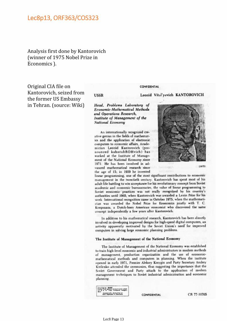
Original CIA file on Kantorovich, seized from the former US Embassy in Tehran. (source: Wiki)
Analysis first done by Kantorovich (winner of 1975 Nobel Prize in Economics ).
Lec8p13, ORF363/COS323
Lec8 Page 13
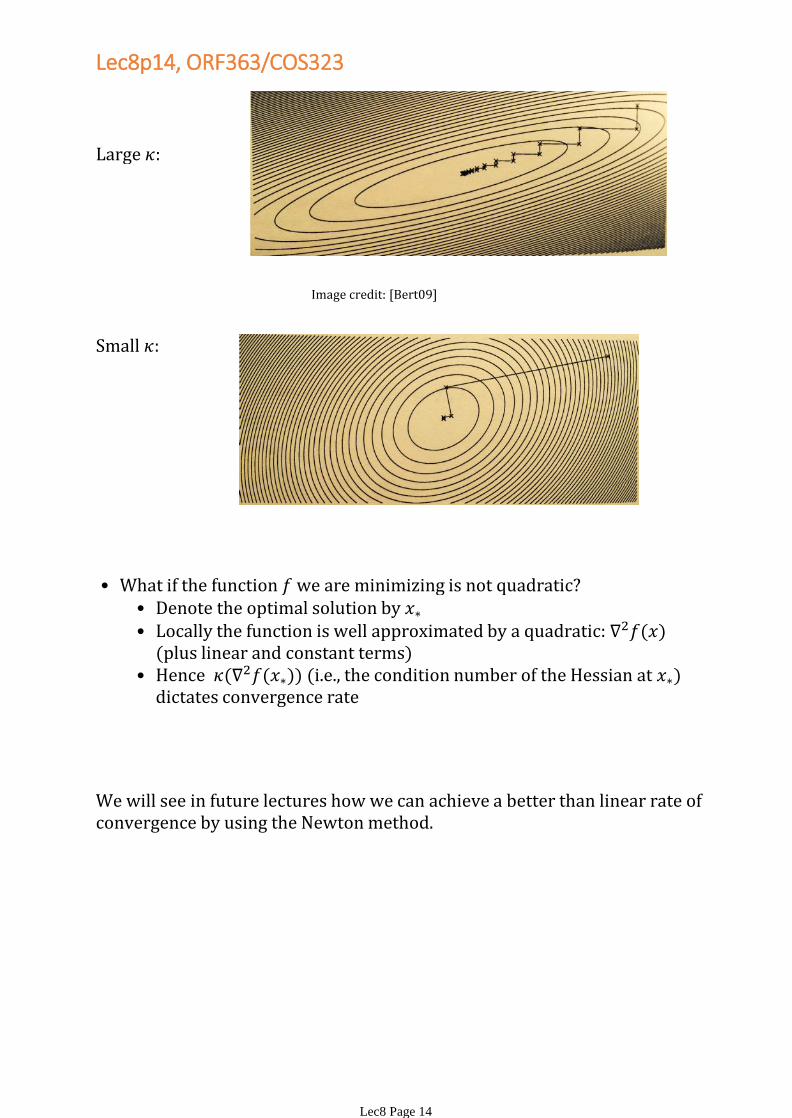
Large
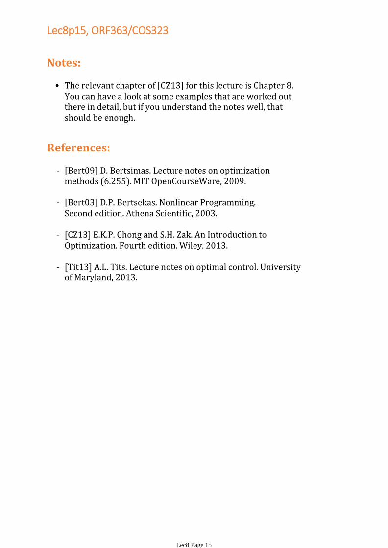
Small
Image credit: [Bert09]
Denote the optimal solution by •Locally the function is well approximated by a quadratic: (plus linear and constant terms)
•
Hence (i.e., the condition number of the Hessian at ) dictates convergence rate
•
What if the function we are minimizing is not quadratic?•
We will see in future lectures how we can achieve a better than linear rate of convergence by using the Newton method.
Lec8p14, ORF363/COS323
Lec8 Page 14
Notes:
The relevant chapter of [CZ13] for this lecture is Chapter 8. You can have a look at some examples that are worked out there in detail, but if you understand the notes well, that should be enough.
•
References:
[Bert09] D. Bertsimas. Lecture notes on optimization methods (6.255). MIT OpenCourseWare, 2009.
-
[Bert03] D.P. Bertsekas. Nonlinear Programming.Second edition. Athena Scientific, 2003.
-
[CZ13] E.K.P. Chong and S.H. Zak. An Introduction to Optimization. Fourth edition. Wiley, 2013.
-
[Tit13] A.L. Tits. Lecture notes on optimal control. University of Maryland, 2013.
-
Lec8p15, ORF363/COS323
Lec8 Page 15


![Lec8p1, ORF363/COS323 - Princeton Universityand Goldstein rule (see, e.g., Section 7.8 of [CZ13]). We will cover Armijo in the next lecture. • Try to ensure enough decrease in line](https://img.pdfslide.net/doc/110x75/5ea70631682dc05c89134fc2/lec8p1-orf363cos323-princeton-and-goldstein-rule-see-eg-section-78-of.jpg)


![Lec3p1, ORF363/COS323 · See, e.g., Theorem 3.7 in Section 3.4 of [CZ13]. Examples: MATLAB: eig([2 4;4 5]) Recall our easy test in dimension 2: This generalizes to n dimensions using](https://img.pdfslide.net/doc/110x75/5fbe7126b9248435bd3cb438/lec3p1-orf363-see-eg-theorem-37-in-section-34-of-cz13-examples-matlab.jpg)