Embed Size (px)
Citation preview
1 © ANSYS, Inc.
Lecture 05: Co-Simulation Solution Process and Postprocessing
ANSYS Fluent Fluid Structure Interaction (FSI) with ANSYS Mechanical
19.0 Release
2 © ANSYS, Inc.
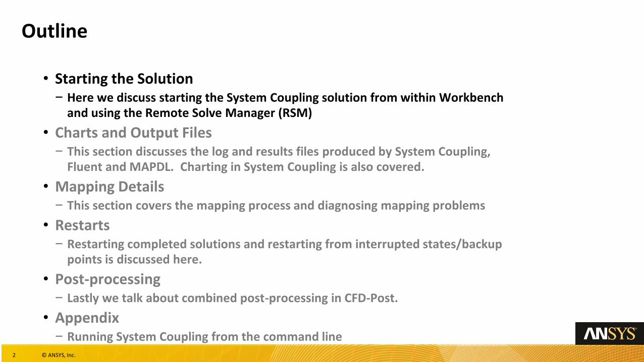
Outline
• Starting the Solution− Here we discuss starting the System Coupling solution from within Workbench
and using the Remote Solve Manager (RSM)
• Charts and Output Files− This section discusses the log and results files produced by System Coupling,
Fluent and MAPDL. Charting in System Coupling is also covered.
• Mapping Details− This section covers the mapping process and diagnosing mapping problems
• Restarts− Restarting completed solutions and restarting from interrupted states/backup
points is discussed here.
• Post-processing− Lastly we talk about combined post-processing in CFD-Post.
• Appendix− Running System Coupling from the command line
3 © ANSYS, Inc.
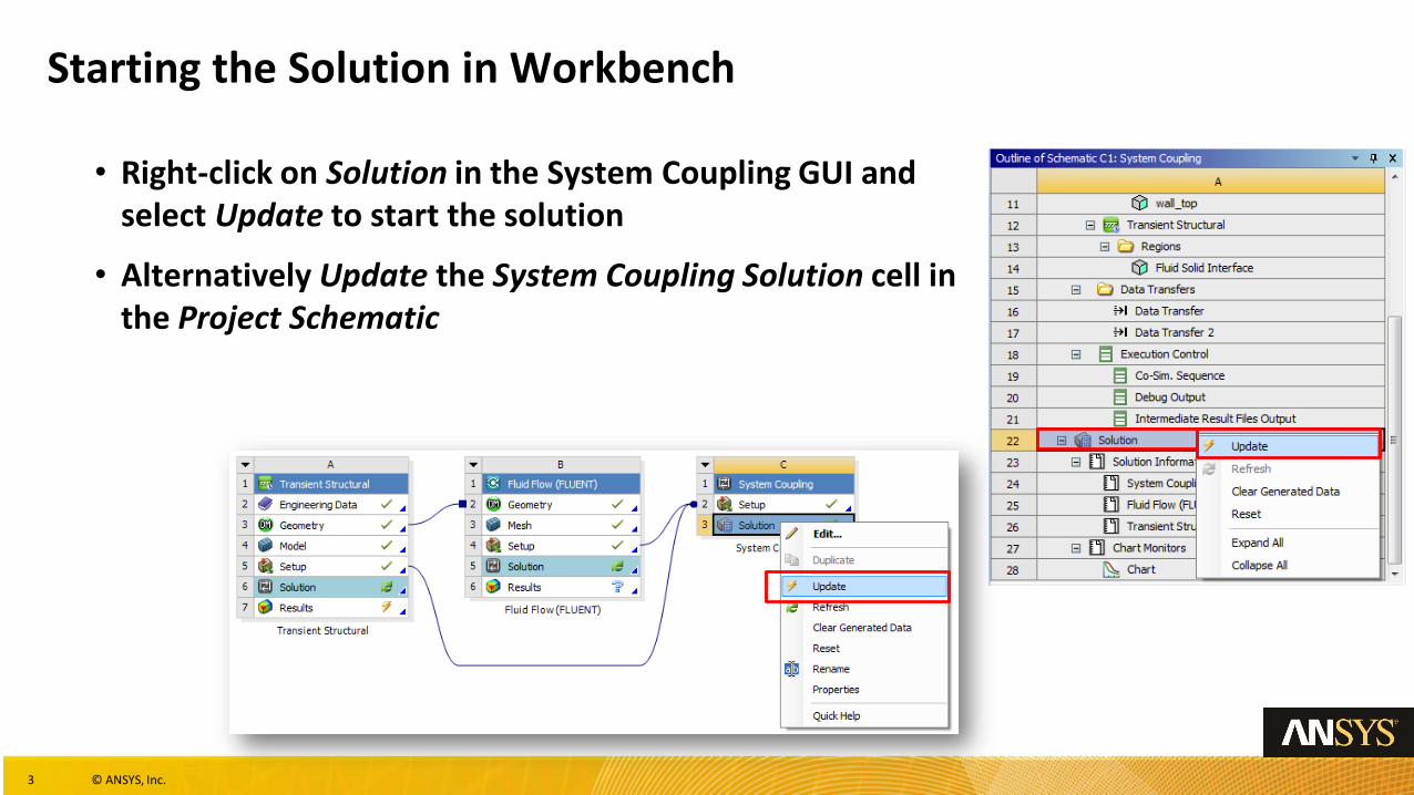
Starting the Solution in Workbench
• Right-click on Solution in the System Coupling GUI and select Update to start the solution
• Alternatively Update the System Coupling Solution cell in the Project Schematic
4 © ANSYS, Inc.
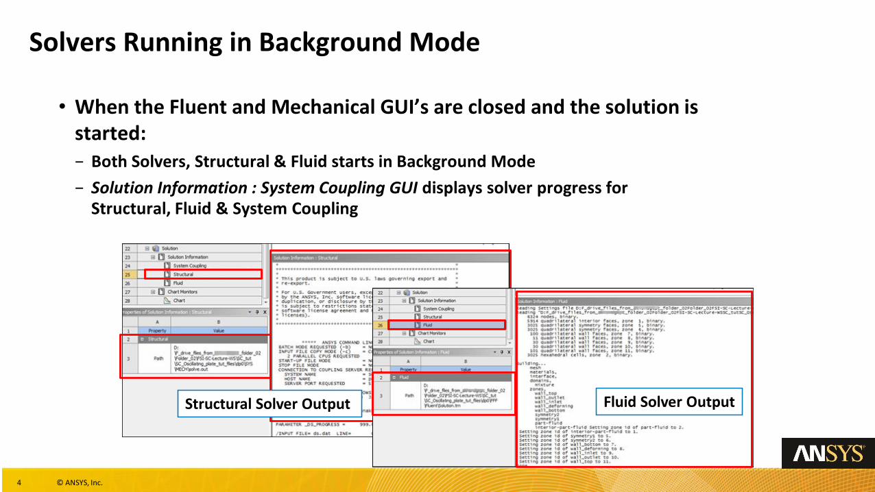
Structural Solver Output
Solvers Running in Background Mode
• When the Fluent and Mechanical GUI’s are closed and the solution is started:− Both Solvers, Structural & Fluid starts in Background Mode
− Solution Information : System Coupling GUI displays solver progress for Structural, Fluid & System Coupling
Fluid Solver Output
5 © ANSYS, Inc.
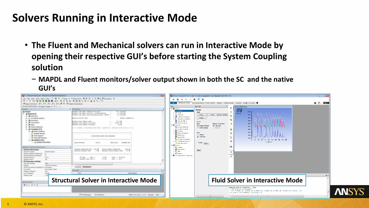
Solvers Running in Interactive Mode
• The Fluent and Mechanical solvers can run in Interactive Mode by opening their respective GUI’s before starting the System Coupling solution− MAPDL and Fluent monitors/solver output shown in both the SC and the native
GUI’s
Structural Solver in Interactive Mode Fluid Solver in Interactive Mode
6 © ANSYS, Inc.
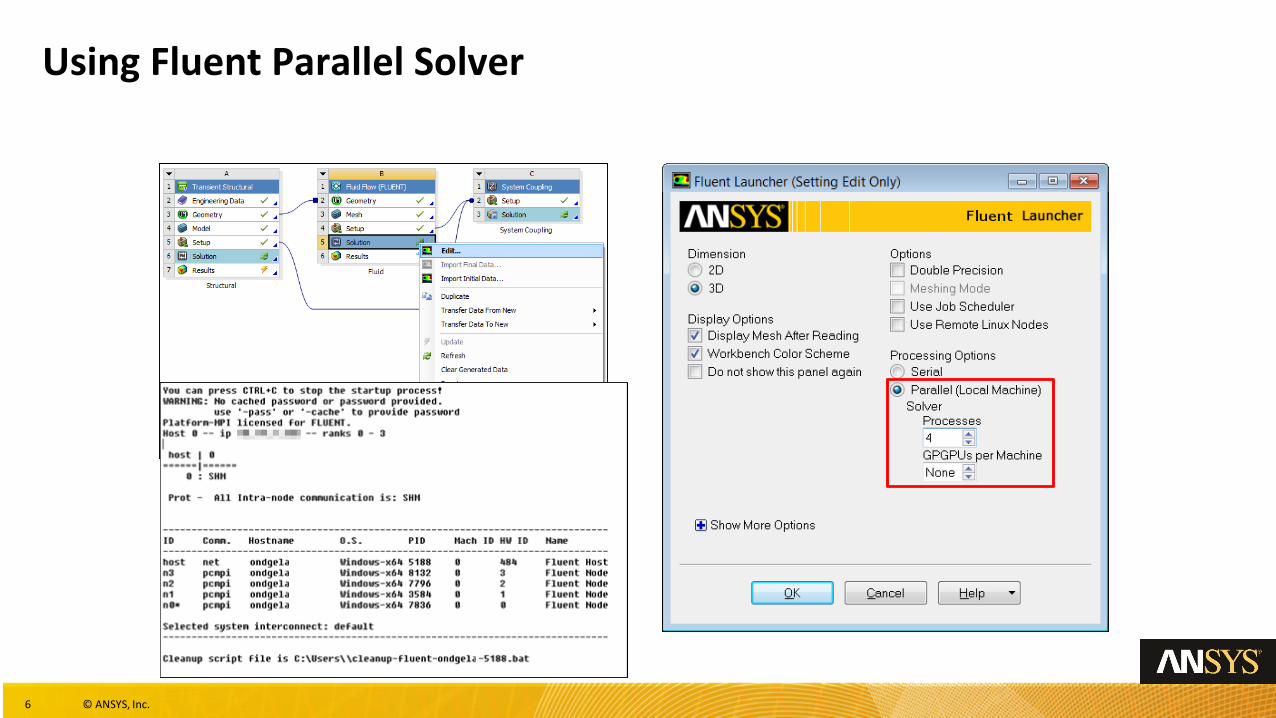
Using Fluent Parallel Solver
7 © ANSYS, Inc.
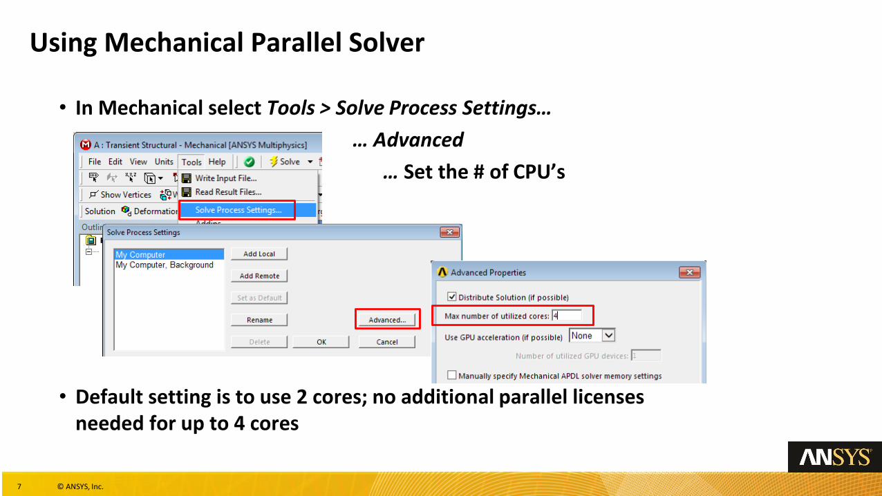
Using Mechanical Parallel Solver
• In Mechanical select Tools > Solve Process Settings…
… Advanced
… Set the # of CPU’s
• Default setting is to use 2 cores; no additional parallel licenses needed for up to 4 cores

8 © ANSYS, Inc.
Core Assignment for Parallel Solvers
• The Fluent and MAPDL solvers can generally share cores if you have sufficient RAM− E.g. if you have an 8 core machine, 8 for Fluent and 6 for MAPDL is OK
− When Fluent is solving and MAPDL is idle, the MAPDL solver processes will use almost no CPU
− When MAPDL is solving and Fluent is idle, the Fluent solver slave processes will use a small amount of CPU (perhaps 5%)
9 © ANSYS, Inc.
Optimizing Solution Times
• Transient 2-way FSI cases can run for a long time− Using too many Coupling Iterations will greatly increase solution time
− Optimizing coupling convergence through appropriate under relaxation factors, time step sizes and Solution Stabilization controls can greatly reduce run times – see the Convergence chapter
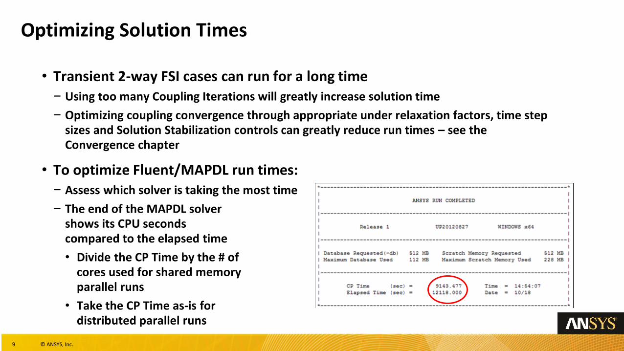
• To optimize Fluent/MAPDL run times:− Assess which solver is taking the most time
− The end of the MAPDL solvershows its CPU secondscompared to the elapsed time
• Divide the CP Time by the # ofcores used for shared memoryparallel runs
• Take the CP Time as-is fordistributed parallel runs
10 © ANSYS, Inc.
Optimizing Solution Times
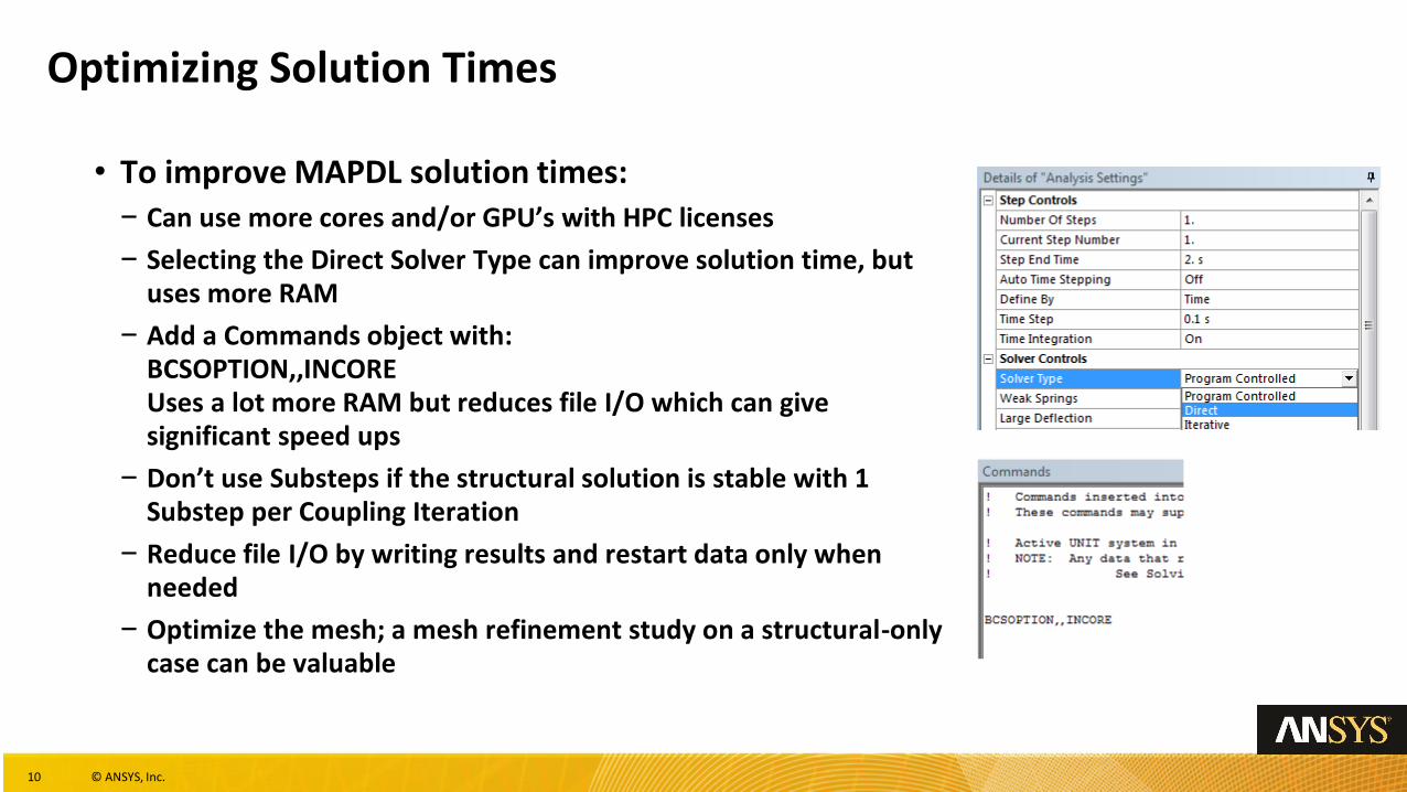
• To improve MAPDL solution times:− Can use more cores and/or GPU’s with HPC licenses
− Selecting the Direct Solver Type can improve solution time, but uses more RAM
− Add a Commands object with:BCSOPTION,,INCOREUses a lot more RAM but reduces file I/O which can give significant speed ups
− Don’t use Substeps if the structural solution is stable with 1 Substep per Coupling Iteration
− Reduce file I/O by writing results and restart data only when needed
− Optimize the mesh; a mesh refinement study on a structural-only case can be valuable
11 © ANSYS, Inc.
Optimizing Solution Times
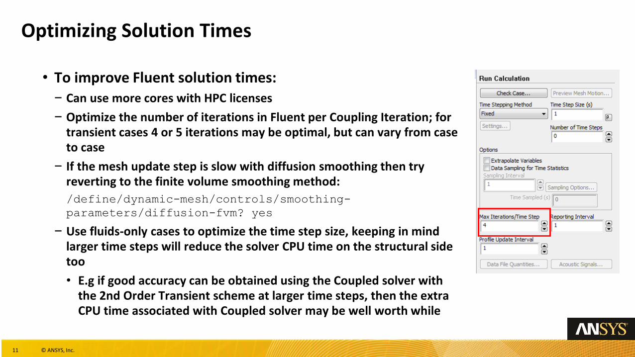
• To improve Fluent solution times:− Can use more cores with HPC licenses
− Optimize the number of iterations in Fluent per Coupling Iteration; for transient cases 4 or 5 iterations may be optimal, but can vary from case to case
− If the mesh update step is slow with diffusion smoothing then try reverting to the finite volume smoothing method:
/define/dynamic-mesh/controls/smoothing-
parameters/diffusion-fvm? yes
− Use fluids-only cases to optimize the time step size, keeping in mind larger time steps will reduce the solver CPU time on the structural side too
• E.g if good accuracy can be obtained using the Coupled solver with the 2nd Order Transient scheme at larger time steps, then the extra CPU time associated with Coupled solver may be well worth while
12 © ANSYS, Inc.
Using the Remote Solve Manager (RSM)
• Project Update via RSM available• Works for all supported queues/cluster
• System coupling log file can be monitored on client machine during run
• Limited control over core assignments
• The Project Update method sends the entire WB project to the remote machine then executes a Project Update• This ensures the Fluent, Mechanical and System Coupling components all start
solving at the same time
• Component submission to RSM (i.e. update only the System Coupling Solution cell) is not available
13 © ANSYS, Inc.
Using the Remote Solve Manager (RSM)
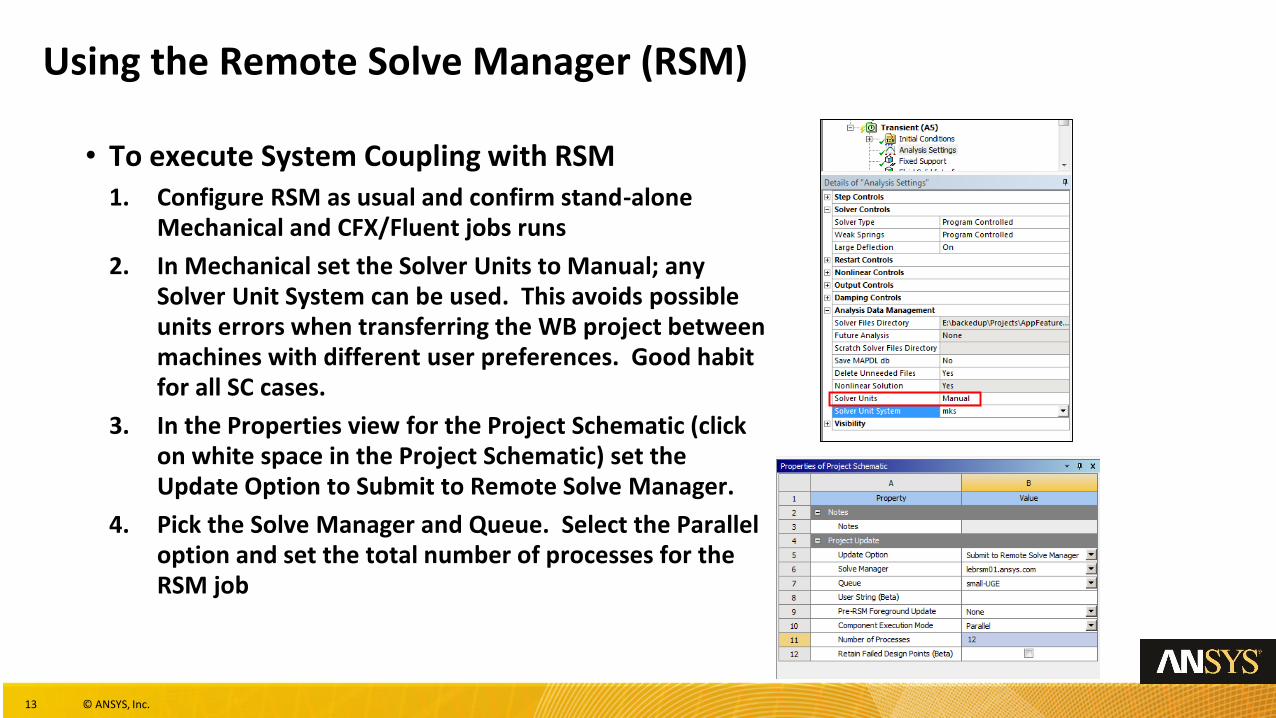
• To execute System Coupling with RSM1. Configure RSM as usual and confirm stand-alone
Mechanical and CFX/Fluent jobs runs
2. In Mechanical set the Solver Units to Manual; any Solver Unit System can be used. This avoids possible units errors when transferring the WB project between machines with different user preferences. Good habit for all SC cases.
3. In the Properties view for the Project Schematic (click on white space in the Project Schematic) set the Update Option to Submit to Remote Solve Manager.
4. Pick the Solve Manager and Queue. Select the Parallel option and set the total number of processes for the RSM job
14 © ANSYS, Inc.
Using the Remote Solve Manager (RSM)
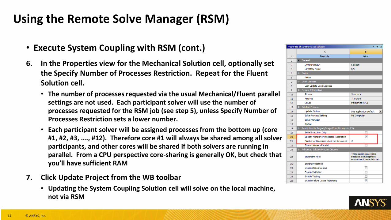
• Execute System Coupling with RSM (cont.)
6. In the Properties view for the Mechanical Solution cell, optionally set the Specify Number of Processes Restriction. Repeat for the Fluent Solution cell.
• The number of processes requested via the usual Mechanical/Fluent parallel settings are not used. Each participant solver will use the number of processes requested for the RSM job (see step 5), unless Specify Number of Processes Restriction sets a lower number.
• Each participant solver will be assigned processes from the bottom up (core #1, #2, #3, …., #12). Therefore core #1 will always be shared among all solver participants, and other cores will be shared if both solvers are running in parallel. From a CPU perspective core-sharing is generally OK, but check that you’ll have sufficient RAM
7. Click Update Project from the WB toolbar
• Updating the System Coupling Solution cell will solve on the local machine, not via RSM
15 © ANSYS, Inc.
Outline
• Starting the Solution− Here we discuss starting the System Coupling solution from within Workbench
and using the Remote Solve Manager (RSM)
• Charts and Output Files− This section discusses the log and results files produced by System Coupling,
Fluent and MAPDL. Charting in System Coupling is also covered.
• Mapping Details− This section covers the mapping process and diagnosing mapping problems
• Restarts− Restarting completed solutions and restarting from interrupted states/backup
points is discussed here.
• Post-processing− Lastly we talk about combined post-processing in CFD-Post.
• Appendix− Running System Coupling from the command line
16 © ANSYS, Inc.
System Coupling Log File
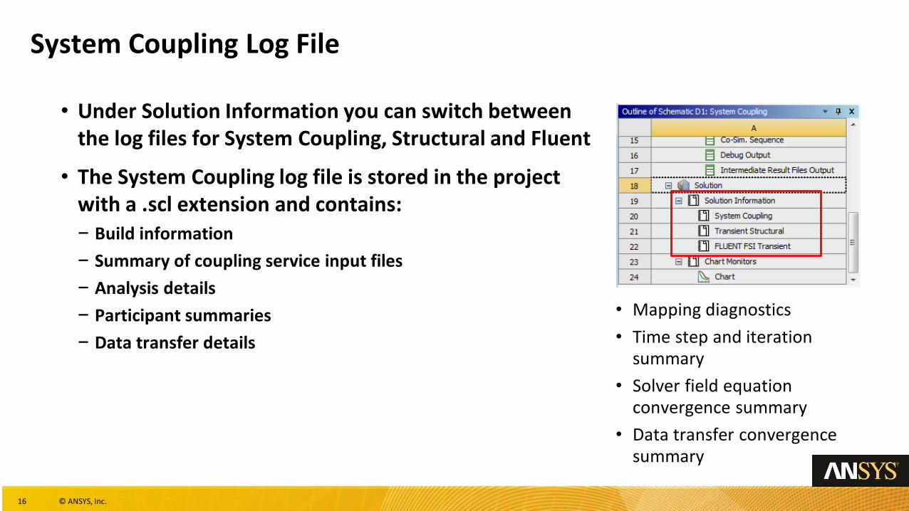
• Under Solution Information you can switch between the log files for System Coupling, Structural and Fluent
• The System Coupling log file is stored in the project with a .scl extension and contains:− Build information
− Summary of coupling service input files
− Analysis details
− Participant summaries
− Data transfer details
• Mapping diagnostics
• Time step and iteration summary
• Solver field equation convergence summary
• Data transfer convergence summary
17 © ANSYS, Inc.
System Coupling Log File
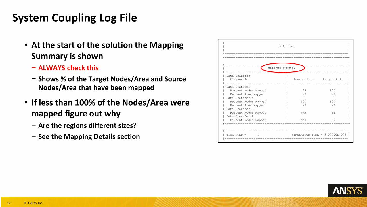
• At the start of the solution the Mapping Summary is shown− ALWAYS check this
− Shows % of the Target Nodes/Area and Source Nodes/Area that have been mapped
• If less than 100% of the Nodes/Area were mapped figure out why− Are the regions different sizes?
− See the Mapping Details section
| |
| Solution |
| |
+====================================================================+
======================================================================
+--------------------------------------------------------------------+
| MAPPING SUMMARY |
+--------------------------------------------------------------------+
| Data Transfer | |
| Diagnostic | Source Side Target Side |
+----------------------------------+---------------------------------+
| Data Transfer | |
| Percent Nodes Mapped | 99 100 |
| Percent Area Mapped | 98 98 |
| Data Transfer 4 | |
| Percent Nodes Mapped | 100 100 |
| Percent Area Mapped | 99 99 |
| Data Transfer 3 | |
| Percent Nodes Mapped | N/A 96 |
| Data Transfer 2 | |
| Percent Nodes Mapped | N/A 99 |
+--------------------------------------------------------------------+
+====================================================================+
| TIME STEP = 1 SIMULATION TIME = 5.00000E-005 |
|--------------------------------------------------------------------|
18 © ANSYS, Inc.
Fluent Transcript (.trn) File
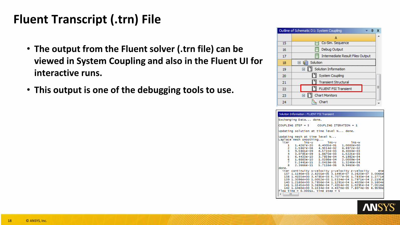
• The output from the Fluent solver (.trn file) can be viewed in System Coupling and also in the Fluent UI for interactive runs.
• This output is one of the debugging tools to use.
19 © ANSYS, Inc.
MAPDL Solver Output File
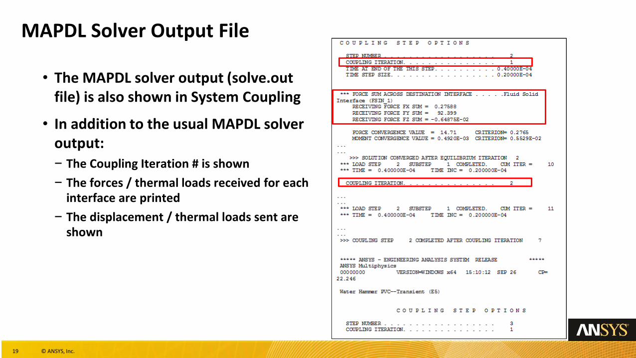
• The MAPDL solver output (solve.outfile) is also shown in System Coupling
• In addition to the usual MAPDL solver output:− The Coupling Iteration # is shown
− The forces / thermal loads received for each interface are printed
− The displacement / thermal loads sent are shown
20 © ANSYS, Inc.
Charts in System Coupling
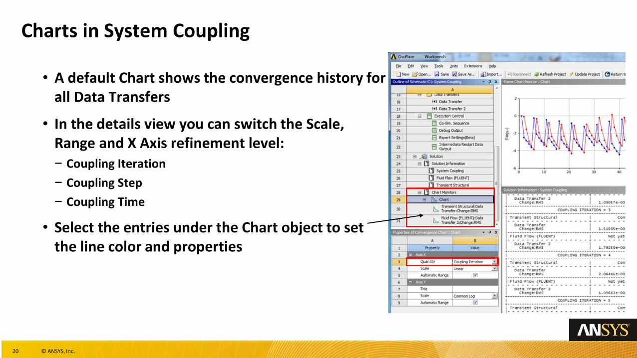
• A default Chart shows the convergence history for all Data Transfers
• In the details view you can switch the Scale, Range and X Axis refinement level:− Coupling Iteration
− Coupling Step
− Coupling Time
• Select the entries under the Chart object to set the line color and properties
21 © ANSYS, Inc.
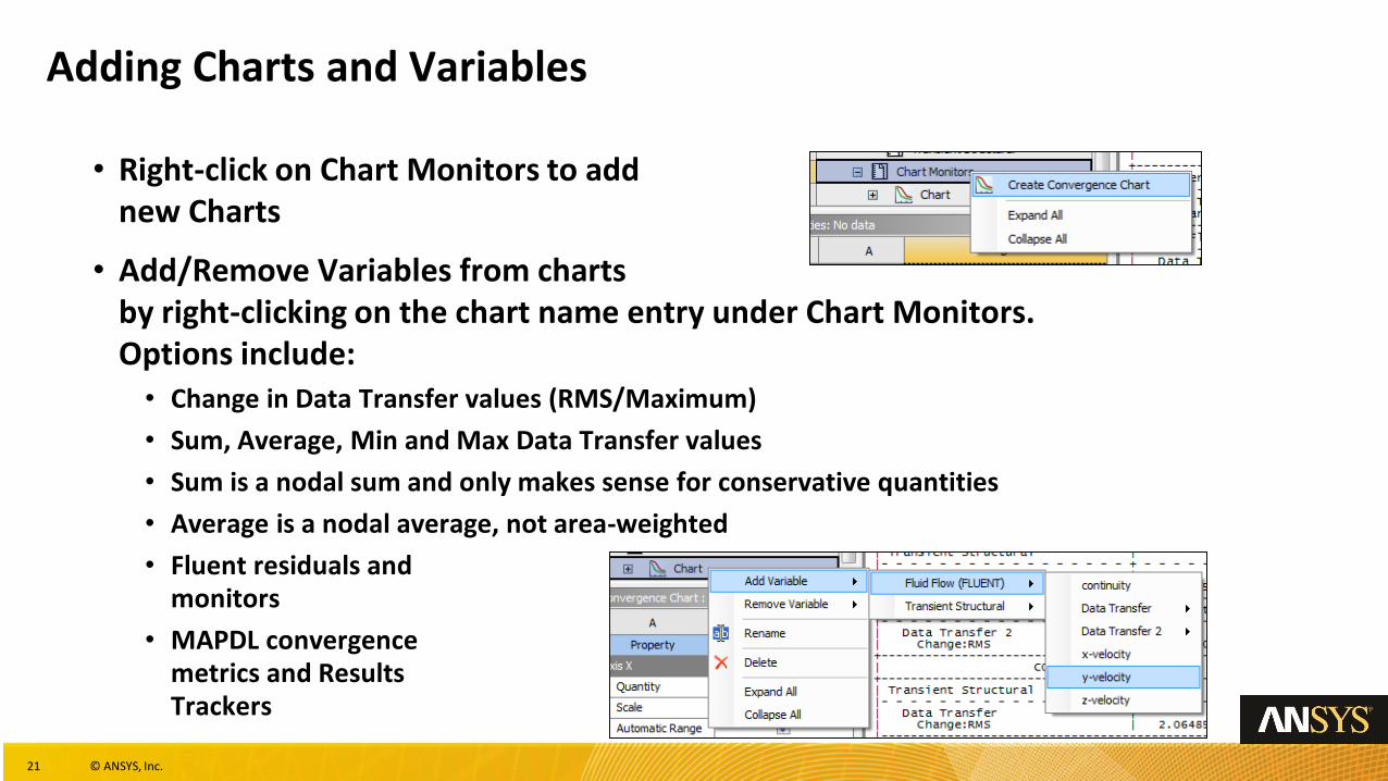
Adding Charts and Variables
• Right-click on Chart Monitors to addnew Charts
• Add/Remove Variables from chartsby right-clicking on the chart name entry under Chart Monitors. Options include:• Change in Data Transfer values (RMS/Maximum)
• Sum, Average, Min and Max Data Transfer values
• Sum is a nodal sum and only makes sense for conservative quantities
• Average is a nodal average, not area-weighted
• Fluent residuals andmonitors
• MAPDL convergencemetrics and ResultsTrackers
22 © ANSYS, Inc.
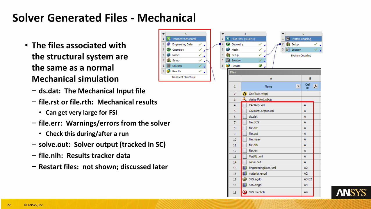
Solver Generated Files - Mechanical
• The files associated withthe structural system arethe same as a normalMechanical simulation− ds.dat: The Mechanical Input file
− file.rst or file.rth: Mechanical results
• Can get very large for FSI
− file.err: Warnings/errors from the solver
• Check this during/after a run
− solve.out: Solver output (tracked in SC)
− file.nlh: Results tracker data
− Restart files: not shown; discussed later
23 © ANSYS, Inc.
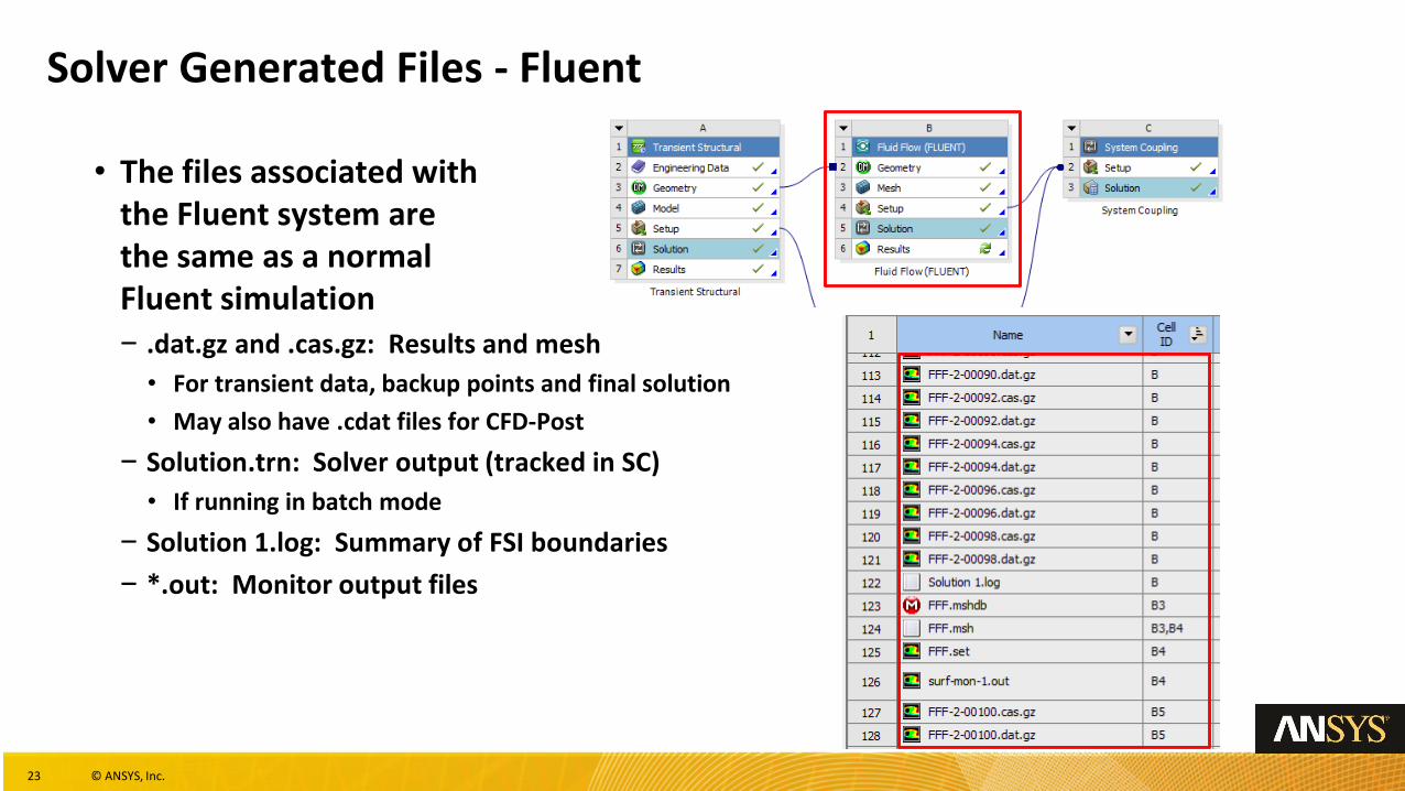
Solver Generated Files - Fluent
• The files associated withthe Fluent system arethe same as a normalFluent simulation− .dat.gz and .cas.gz: Results and mesh
• For transient data, backup points and final solution
• May also have .cdat files for CFD-Post
− Solution.trn: Solver output (tracked in SC)
• If running in batch mode
− Solution 1.log: Summary of FSI boundaries
− *.out: Monitor output files
24 © ANSYS, Inc.
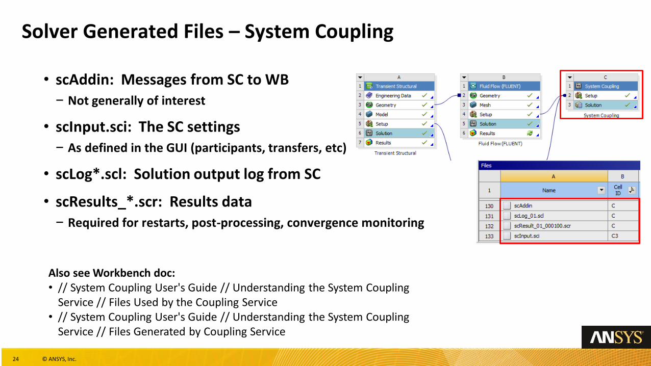
Solver Generated Files – System Coupling
• scAddin: Messages from SC to WB− Not generally of interest
• scInput.sci: The SC settings− As defined in the GUI (participants, transfers, etc)
• scLog*.scl: Solution output log from SC
• scResults_*.scr: Results data− Required for restarts, post-processing, convergence monitoring
Also see Workbench doc:• // System Coupling User's Guide // Understanding the System Coupling
Service // Files Used by the Coupling Service• // System Coupling User's Guide // Understanding the System Coupling
Service // Files Generated by Coupling Service
25 © ANSYS, Inc.
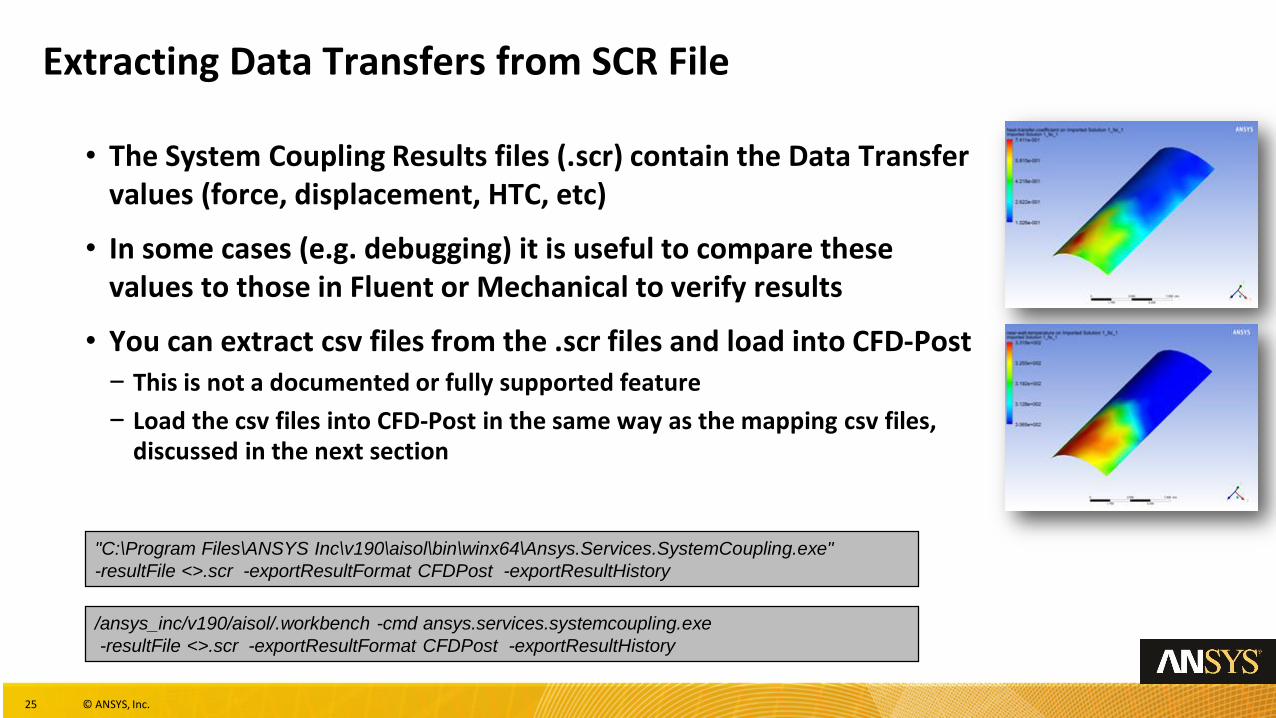
Extracting Data Transfers from SCR File
• The System Coupling Results files (.scr) contain the Data Transfer values (force, displacement, HTC, etc)
• In some cases (e.g. debugging) it is useful to compare these values to those in Fluent or Mechanical to verify results
• You can extract csv files from the .scr files and load into CFD-Post− This is not a documented or fully supported feature
− Load the csv files into CFD-Post in the same way as the mapping csv files, discussed in the next section
"C:\Program Files\ANSYS Inc\v190\aisol\bin\winx64\Ansys.Services.SystemCoupling.exe"
-resultFile <>.scr -exportResultFormat CFDPost -exportResultHistory
/ansys_inc/v190/aisol/.workbench -cmd ansys.services.systemcoupling.exe
-resultFile <>.scr -exportResultFormat CFDPost -exportResultHistory
26 © ANSYS, Inc.
Outline
• Starting the Solution− Here we discuss starting the System Coupling solution from within Workbench
and using the Remote Solve Manager (RSM)
• Charts and Output Files− This section discusses the log and results files produced by System Coupling,
Fluent and MAPDL. Charting in System Coupling is also covered.
• Mapping Details− This section covers the mapping process and diagnosing mapping problems
• Restarts− Restarting completed solutions and restarting from interrupted states/backup
points is discussed here.
• Post-processing− Lastly we talk about combined post-processing in CFD-Post.
• Appendix− Running System Coupling from the command line
27 © ANSYS, Inc.
Data Transfer Process
• Data transfer process consists of :1. Mapping
• This involves the matching of source and target locations to generate mapping weights
• A fluid node must be mapped to a solid element to receive displacements
• Similarly, a solid node or a Gauss integration point in a solid element must be mapped to a fluid element to receive a load
2. Interpolation
• This involves the (re)use of the generated mapping weights to project source data onto target locations
3. Interpolated Data Post-Processing
• This involves possible explicit under relaxation of the target data
28 © ANSYS, Inc.
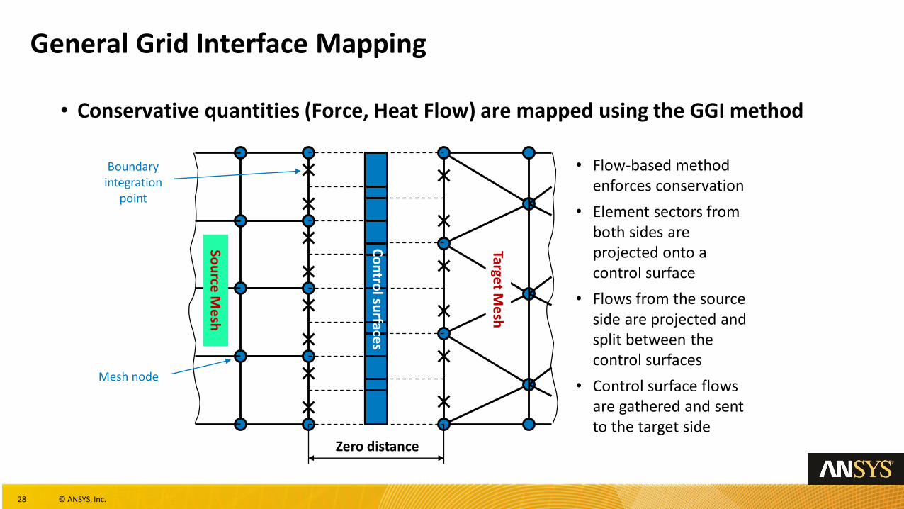
General Grid Interface Mapping
• Conservative quantities (Force, Heat Flow) are mapped using the GGI method
Zero distance
Co
ntro
l surface
s
Sou
rce M
esh
Target M
esh
Mesh node
Boundary integration
point
• Flow-based method enforces conservation
• Element sectors from both sides are projected onto a control surface
• Flows from the source side are projected and split between the control surfaces
• Control surface flows are gathered and sent to the target side
29 © ANSYS, Inc.
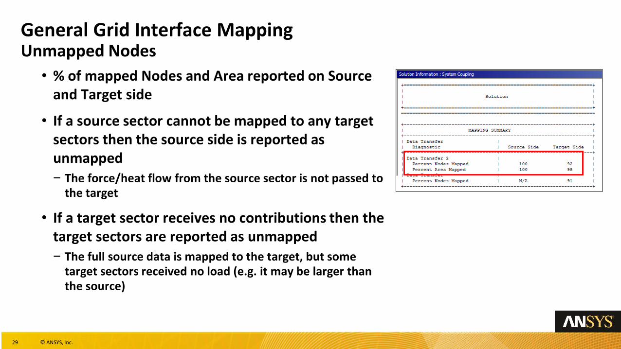
General Grid Interface MappingUnmapped Nodes
• % of mapped Nodes and Area reported on Source and Target side
• If a source sector cannot be mapped to any target sectors then the source side is reported as unmapped− The force/heat flow from the source sector is not passed to
the target
• If a target sector receives no contributions then the target sectors are reported as unmapped− The full source data is mapped to the target, but some
target sectors received no load (e.g. it may be larger than the source)
30 © ANSYS, Inc.
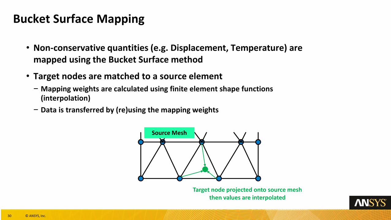
Bucket Surface Mapping
• Non-conservative quantities (e.g. Displacement, Temperature) are mapped using the Bucket Surface method
• Target nodes are matched to a source element− Mapping weights are calculated using finite element shape functions
(interpolation)
− Data is transferred by (re)using the mapping weights
Source Mesh
Target node projected onto source mesh then values are interpolated
31 © ANSYS, Inc.
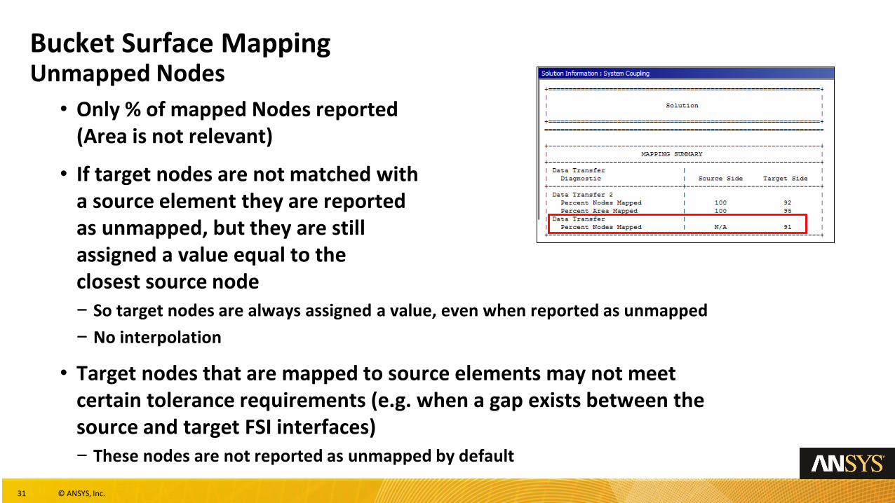
Bucket Surface MappingUnmapped Nodes
• Only % of mapped Nodes reported(Area is not relevant)
• If target nodes are not matched witha source element they are reportedas unmapped, but they are stillassigned a value equal to theclosest source node− So target nodes are always assigned a value, even when reported as unmapped
− No interpolation
• Target nodes that are mapped to source elements may not meet certain tolerance requirements (e.g. when a gap exists between the source and target FSI interfaces)− These nodes are not reported as unmapped by default
32 © ANSYS, Inc.
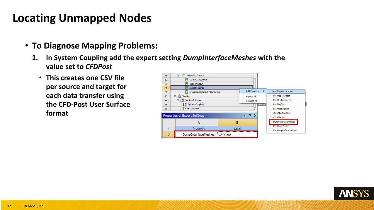
Locating Unmapped Nodes
• To Diagnose Mapping Problems:1. In System Coupling add the expert setting DumpInterfaceMeshes with the
value set to CFDPost
• This creates one CSV fileper source and target foreach data transfer usingthe CFD-Post User Surfaceformat
33 © ANSYS, Inc.
Locating Unmapped Nodes
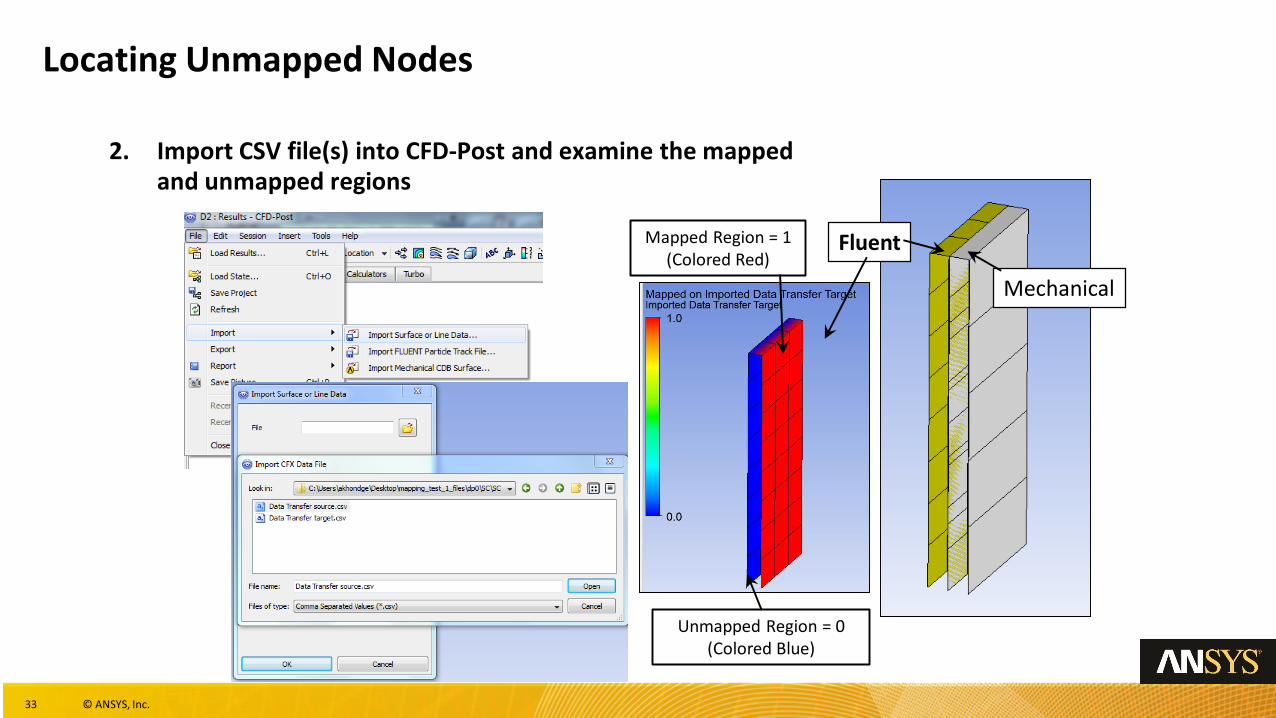
2. Import CSV file(s) into CFD-Post and examine the mapped and unmapped regions
Fluent
Mechanical
Unmapped Region = 0 (Colored Blue)
Mapped Region = 1 (Colored Red)
34 © ANSYS, Inc.
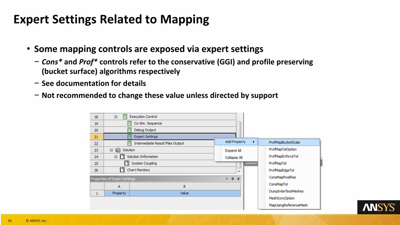
Expert Settings Related to Mapping
• Some mapping controls are exposed via expert settings− Cons* and Prof* controls refer to the conservative (GGI) and profile preserving
(bucket surface) algorithms respectively
− See documentation for details
− Not recommended to change these value unless directed by support
35 © ANSYS, Inc.
Outline
• Starting the Solution− Here we discuss starting the System Coupling solution from within Workbench
and using the Remote Solve Manager (RSM)
• Charts and Output Files− This section discusses the log and results files produced by System Coupling,
Fluent and MAPDL. Charting in System Coupling is also covered.
• Mapping Details− This section covers the mapping process and diagnosing mapping problems
• Restarts− Restarting completed solutions and restarting from interrupted states/backup
points is discussed here.
• Post-processing− Lastly we talk about combined post-processing in CFD-Post.
• Appendix− Running System Coupling from the command line
36 © ANSYS, Inc.
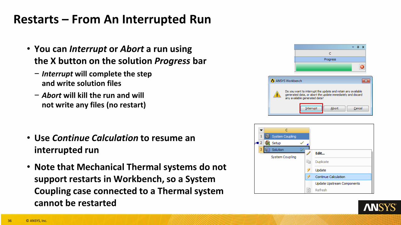
Restarts – From An Interrupted Run
• You can Interrupt or Abort a run usingthe X button on the solution Progress bar− Interrupt will complete the step
and write solution files
− Abort will kill the run and willnot write any files (no restart)
• Use Continue Calculation to resume aninterrupted run
• Note that Mechanical Thermal systems do not support restarts in Workbench, so a System Coupling case connected to a Thermal system cannot be restarted
37 © ANSYS, Inc.
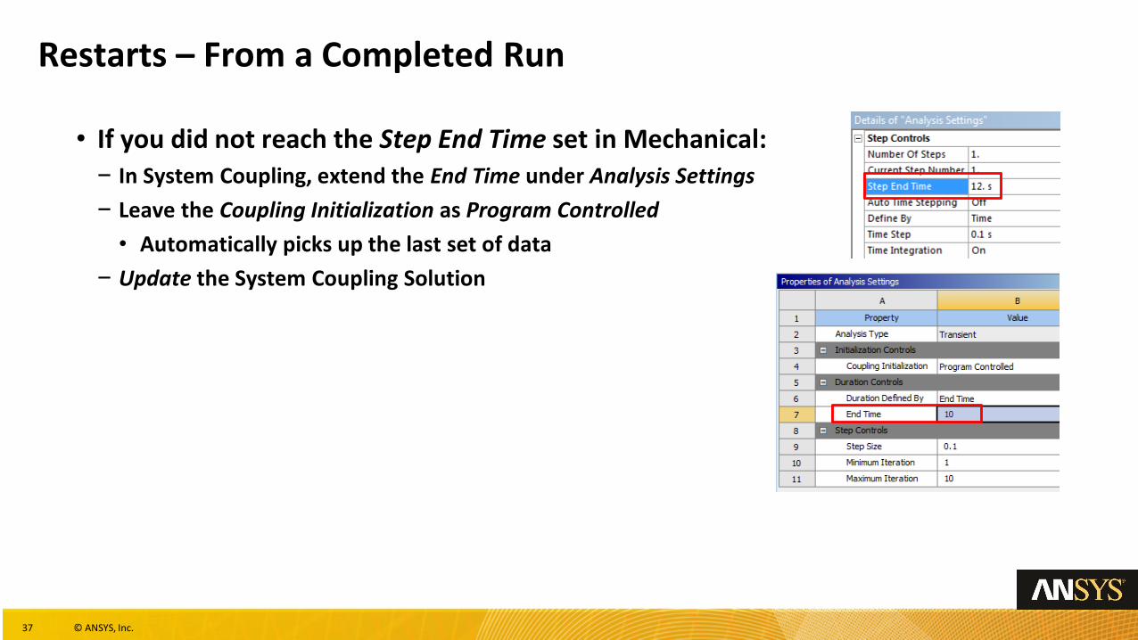
Restarts – From a Completed Run
• If you did not reach the Step End Time set in Mechanical:− In System Coupling, extend the End Time under Analysis Settings
− Leave the Coupling Initialization as Program Controlled
• Automatically picks up the last set of data
− Update the System Coupling Solution
38 © ANSYS, Inc.
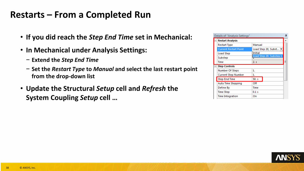
Restarts – From a Completed Run
• If you did reach the Step End Time set in Mechanical:
• In Mechanical under Analysis Settings:− Extend the Step End Time
− Set the Restart Type to Manual and select the last restart point from the drop-down list
• Update the Structural Setup cell and Refresh the System Coupling Setup cell …
39 © ANSYS, Inc.
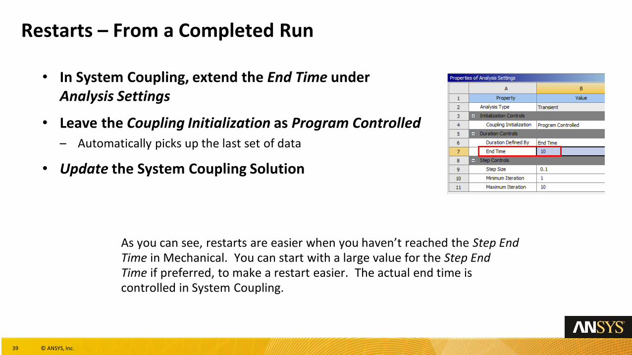
Restarts – From a Completed Run
• In System Coupling, extend the End Time under Analysis Settings
• Leave the Coupling Initialization as Program Controlled– Automatically picks up the last set of data
• Update the System Coupling Solution
As you can see, restarts are easier when you haven’t reached the Step End Time in Mechanical. You can start with a large value for the Step End Time if preferred, to make a restart easier. The actual end time is controlled in System Coupling.
40 © ANSYS, Inc.
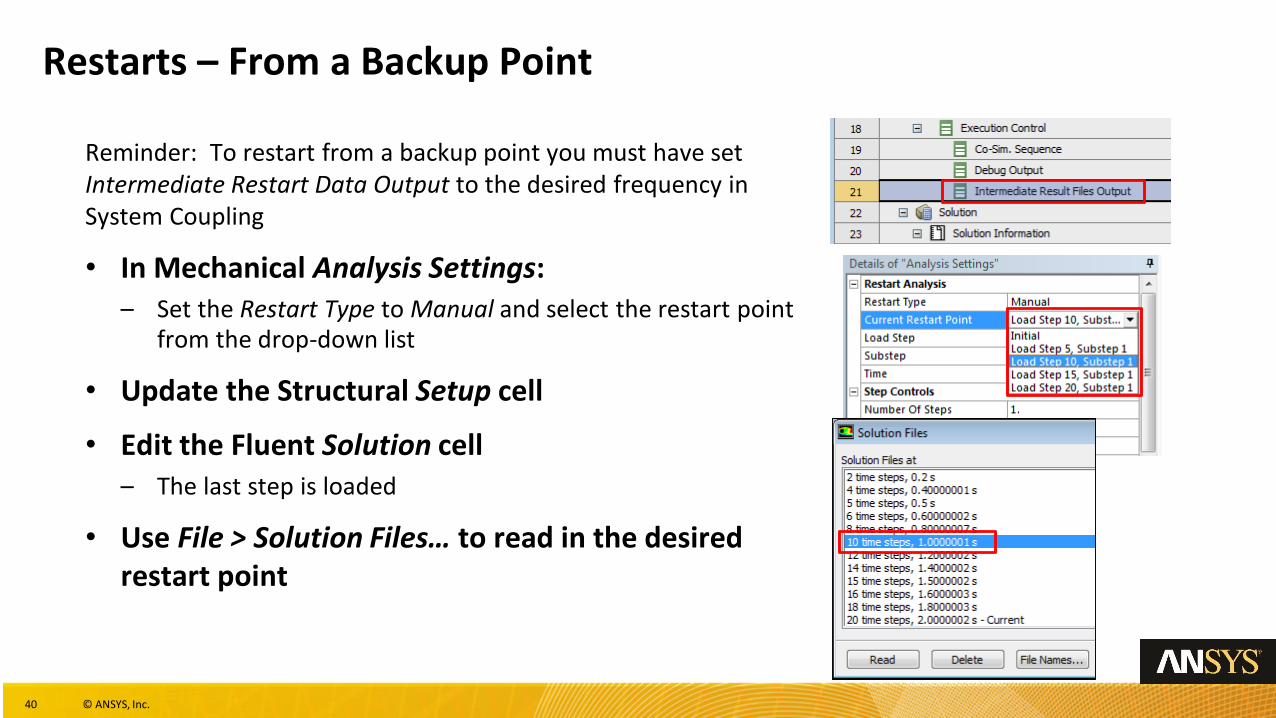
Restarts – From a Backup Point
Reminder: To restart from a backup point you must have set Intermediate Restart Data Output to the desired frequency in System Coupling
• In Mechanical Analysis Settings:– Set the Restart Type to Manual and select the restart point
from the drop-down list
• Update the Structural Setup cell
• Edit the Fluent Solution cell– The last step is loaded
• Use File > Solution Files… to read in the desired restart point
41 © ANSYS, Inc.
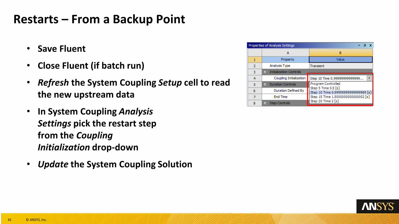
Restarts – From a Backup Point
• Save Fluent
• Close Fluent (if batch run)
• Refresh the System Coupling Setup cell to read the new upstream data
• In System Coupling AnalysisSettings pick the restart stepfrom the CouplingInitialization drop-down
• Update the System Coupling Solution
42 © ANSYS, Inc.
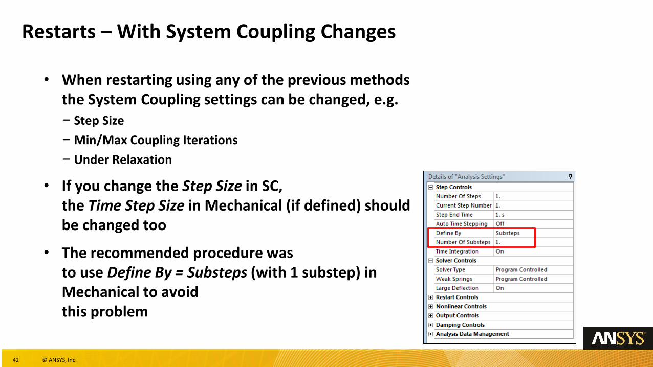
Restarts – With System Coupling Changes
• When restarting using any of the previous methods the System Coupling settings can be changed, e.g.− Step Size
− Min/Max Coupling Iterations
− Under Relaxation
• If you change the Step Size in SC,the Time Step Size in Mechanical (if defined) should be changed too
• The recommended procedure wasto use Define By = Substeps (with 1 substep) in Mechanical to avoidthis problem
43 © ANSYS, Inc.
Restarts – With Mechanical Changes
• When restarting using any of the previous methods the settings in Mechanical can generally be changed, e.g.− Time Integration (to switch between steady-state and transient)
− Constraints and Loads
− Output controls
• Some changes are not supported for restarts (e.g change solver type) and will cause a silent reset of the Mechanical solution data. Get in the habit of saving your project before any restarts so you can revert back if problems occur
• See Mechanical Applications doc:
• // Mechanical User Guide // Understanding Solving // Solution Restarts >> Modifications Affecting Restart Points
44 © ANSYS, Inc.
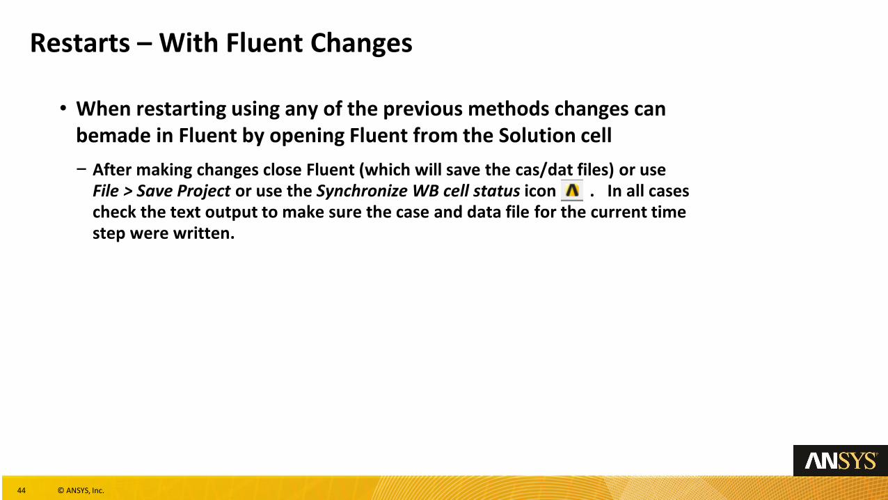
Restarts – With Fluent Changes
• When restarting using any of the previous methods changes can bemade in Fluent by opening Fluent from the Solution cell
− After making changes close Fluent (which will save the cas/dat files) or use File > Save Project or use the Synchronize WB cell status icon . In all cases check the text output to make sure the case and data file for the current time step were written.
45 © ANSYS, Inc.
Crash Recovery
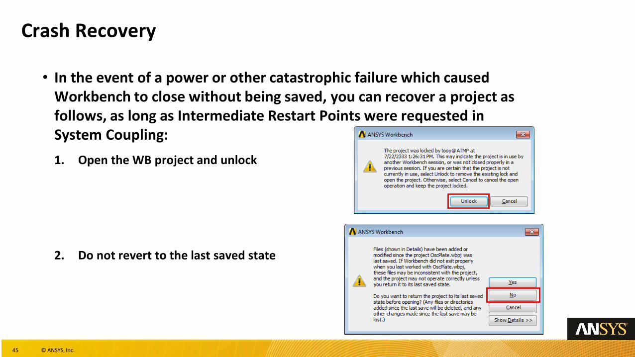
• In the event of a power or other catastrophic failure which caused Workbench to close without being saved, you can recover a project as follows, as long as Intermediate Restart Points were requested in System Coupling:
1. Open the WB project and unlock
2. Do not revert to the last saved state
46 © ANSYS, Inc.
Crash Recovery – Patch Mechanical
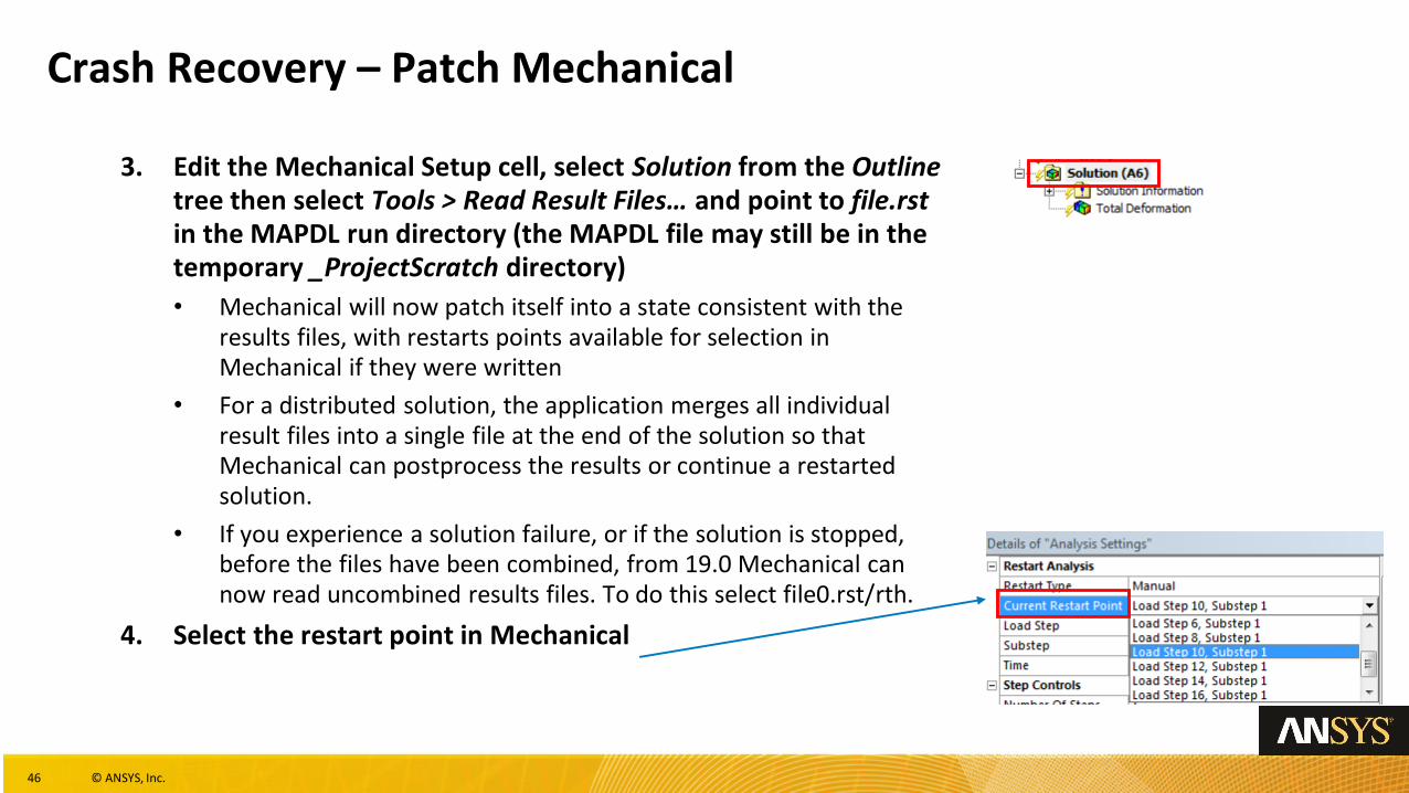
3. Edit the Mechanical Setup cell, select Solution from the Outline tree then select Tools > Read Result Files… and point to file.rstin the MAPDL run directory (the MAPDL file may still be in the temporary _ProjectScratch directory)
• Mechanical will now patch itself into a state consistent with the results files, with restarts points available for selection in Mechanical if they were written
• For a distributed solution, the application merges all individual result files into a single file at the end of the solution so that Mechanical can postprocess the results or continue a restarted solution.
• If you experience a solution failure, or if the solution is stopped, before the files have been combined, from 19.0 Mechanical can now read uncombined results files. To do this select file0.rst/rth.
4. Select the restart point in Mechanical
47 © ANSYS, Inc.
Crash Recovery – Patch Fluent
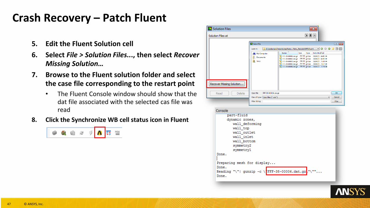
5. Edit the Fluent Solution cell
6. Select File > Solution Files..., then select Recover Missing Solution…
7. Browse to the Fluent solution folder and select the case file corresponding to the restart point
• The Fluent Console window should show that the dat file associated with the selected cas file was read
8. Click the Synchronize WB cell status icon in Fluent
48 © ANSYS, Inc.
Crash Recovery – Patch System Coupling
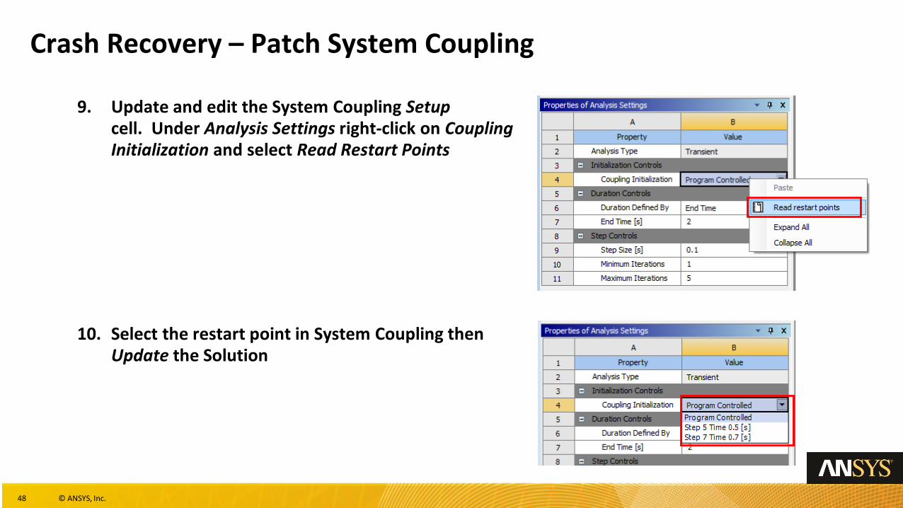
9. Update and edit the System Coupling Setupcell. Under Analysis Settings right-click on Coupling Initialization and select Read Restart Points
10. Select the restart point in System Coupling then Update the Solution
49 © ANSYS, Inc.
Outline
• Starting the Solution− Here we discuss starting the System Coupling solution from within Workbench
and using the Remote Solve Manager (RSM)
• Charts and Output Files− This section discusses the log and results files produced by System Coupling,
Fluent and MAPDL. Charting in System Coupling is also covered.
• Mapping Details− This section covers the mapping process and diagnosing mapping problems
• Restarts− Restarting completed solutions and restarting from interrupted states/backup
points is discussed here.
• Post-processing− Lastly we talk about combined post-processing in CFD-Post.
• Appendix− Running System Coupling from the command line
50 © ANSYS, Inc.
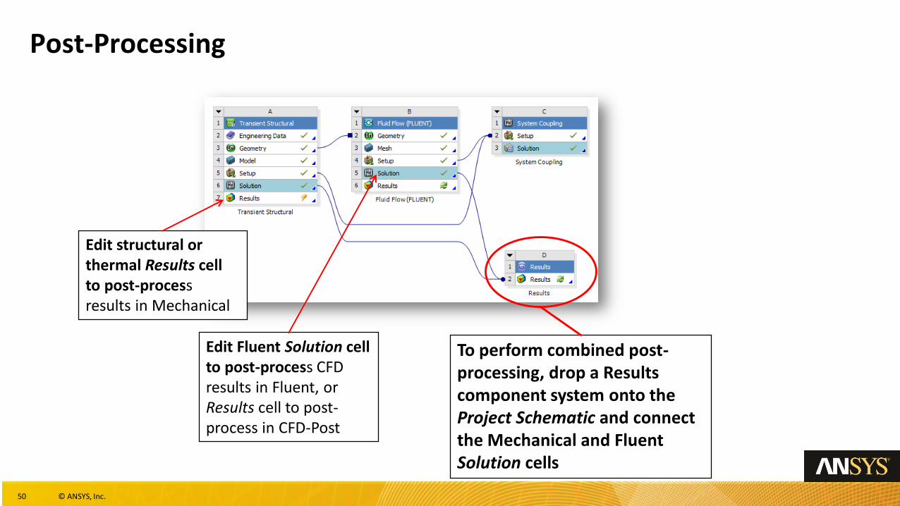
Post-Processing
Edit structural or thermal Results cell to post-process results in Mechanical
Edit Fluent Solution cell to post-process CFD results in Fluent, or Results cell to post-process in CFD-Post
To perform combined post-processing, drop a Results component system onto the Project Schematic and connect the Mechanical and Fluent Solution cells
51 © ANSYS, Inc.
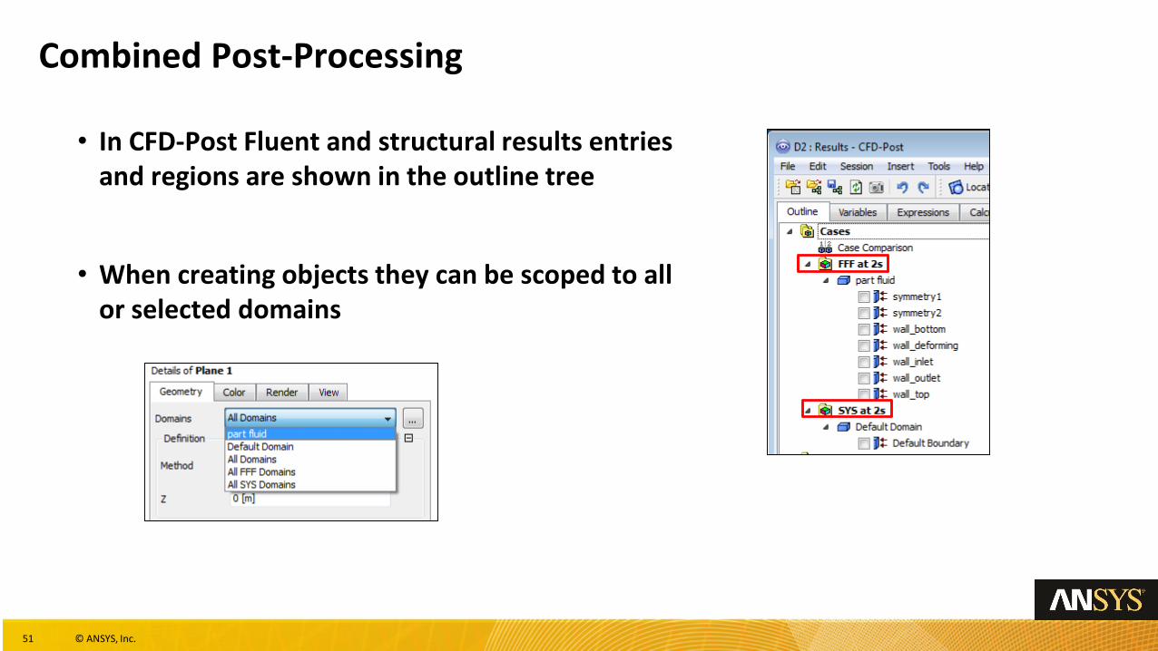
Combined Post-Processing
• In CFD-Post Fluent and structural results entries and regions are shown in the outline tree
• When creating objects they can be scoped to all or selected domains
52 © ANSYS, Inc.
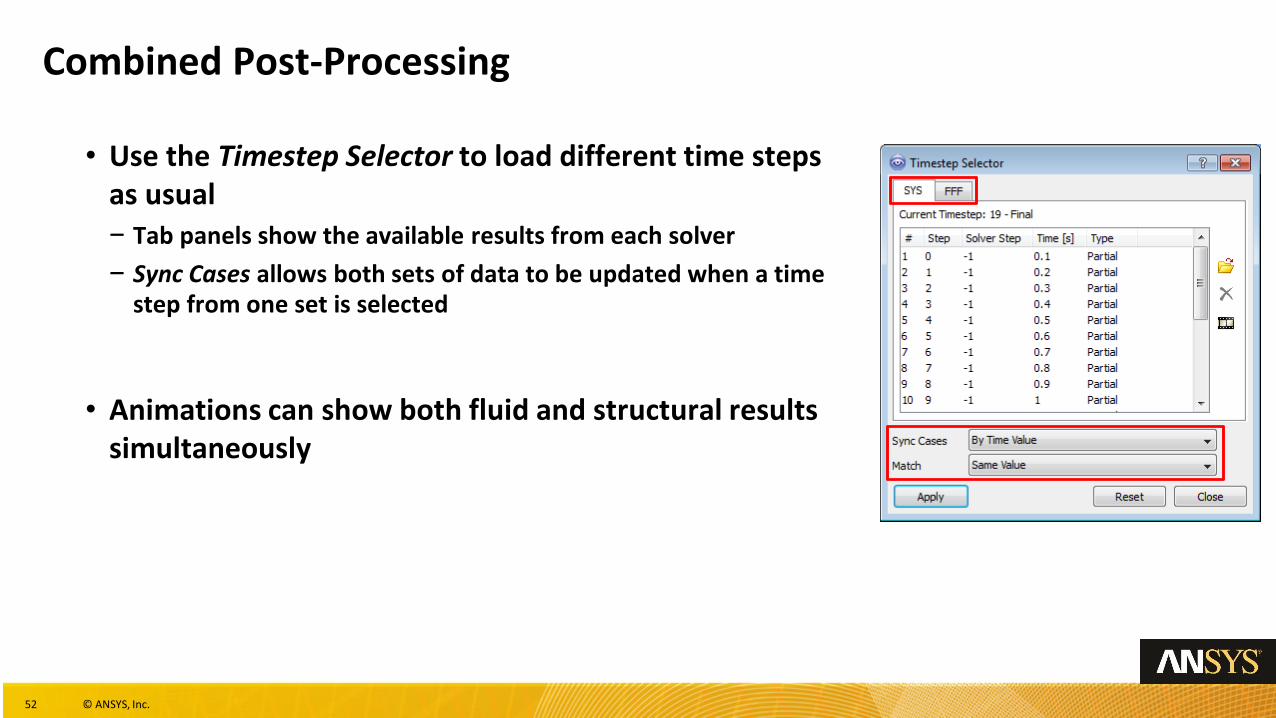
Combined Post-Processing
• Use the Timestep Selector to load different time steps as usual− Tab panels show the available results from each solver
− Sync Cases allows both sets of data to be updated when a time step from one set is selected
• Animations can show both fluid and structural results simultaneously
53 © ANSYS, Inc.
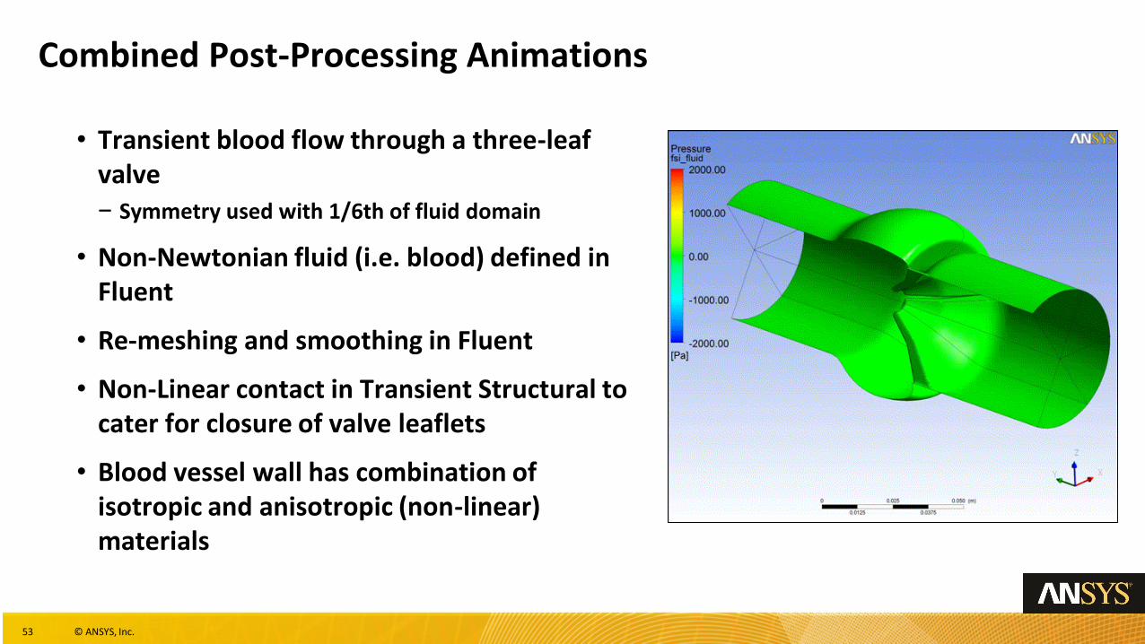
Combined Post-Processing Animations
• Transient blood flow through a three-leaf valve − Symmetry used with 1/6th of fluid domain
• Non-Newtonian fluid (i.e. blood) defined in Fluent
• Re-meshing and smoothing in Fluent
• Non-Linear contact in Transient Structural to cater for closure of valve leaflets
• Blood vessel wall has combination of isotropic and anisotropic (non-linear) materials
54 © ANSYS, Inc.
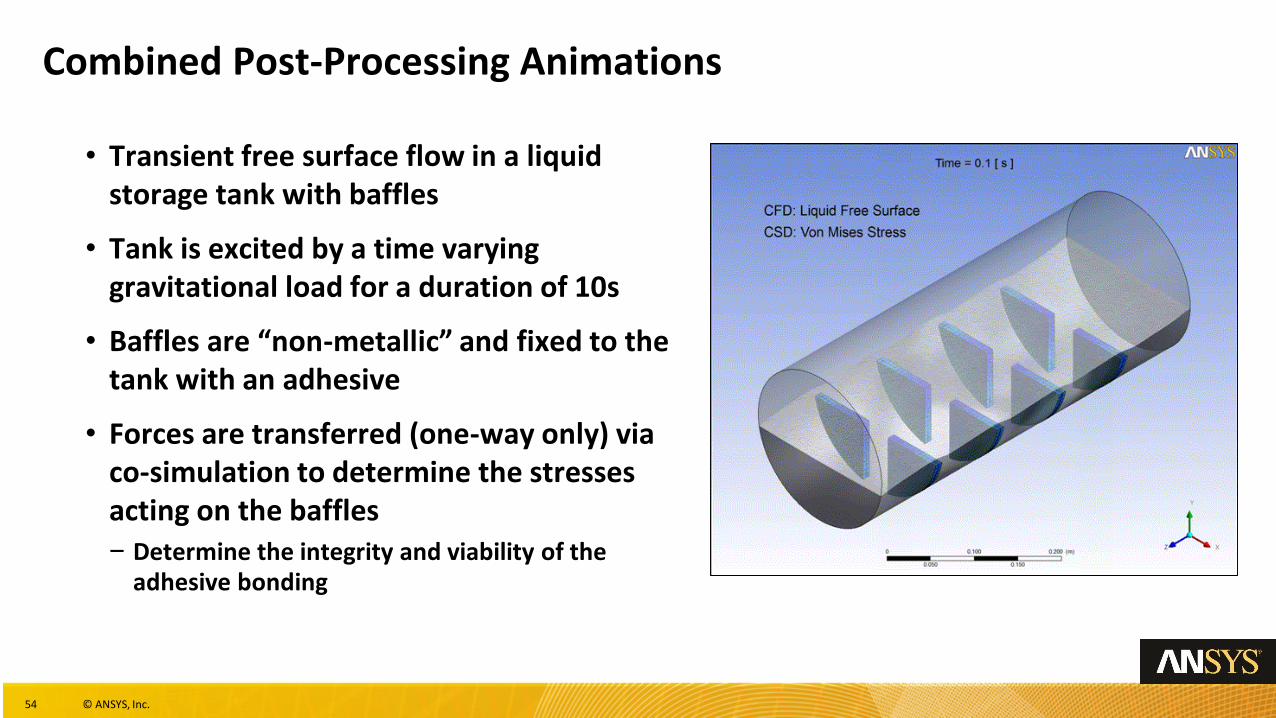
Combined Post-Processing Animations
• Transient free surface flow in a liquid storage tank with baffles
• Tank is excited by a time varying gravitational load for a duration of 10s
• Baffles are “non-metallic” and fixed to the tank with an adhesive
• Forces are transferred (one-way only) via co-simulation to determine the stresses acting on the baffles− Determine the integrity and viability of the
adhesive bonding
55 © ANSYS, Inc.
Combined Post-Processing Animations
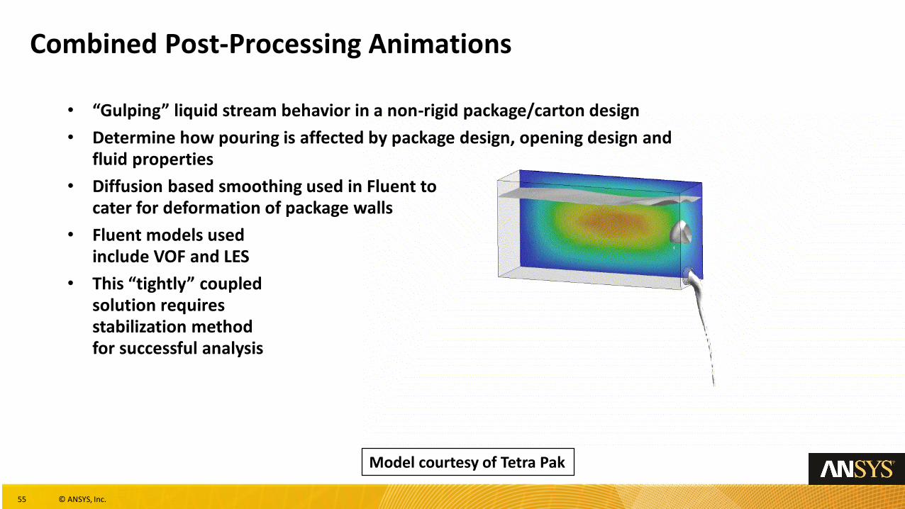
Model courtesy of Tetra Pak
• “Gulping” liquid stream behavior in a non-rigid package/carton design
• Determine how pouring is affected by package design, opening design and fluid properties
• Diffusion based smoothing used in Fluent to cater for deformation of package walls
• Fluent models usedinclude VOF and LES
• This “tightly” coupledsolution requiresstabilization methodfor successful analysis
56 © ANSYS, Inc.
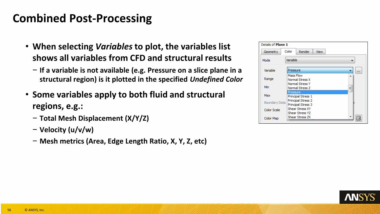
Combined Post-Processing
• When selecting Variables to plot, the variables list shows all variables from CFD and structural results− If a variable is not available (e.g. Pressure on a slice plane in a
structural region) is it plotted in the specified Undefined Color
• Some variables apply to both fluid and structural regions, e.g.:− Total Mesh Displacement (X/Y/Z)
− Velocity (u/v/w)
− Mesh metrics (Area, Edge Length Ratio, X, Y, Z, etc)
57 © ANSYS, Inc.
Combined Post-Processing
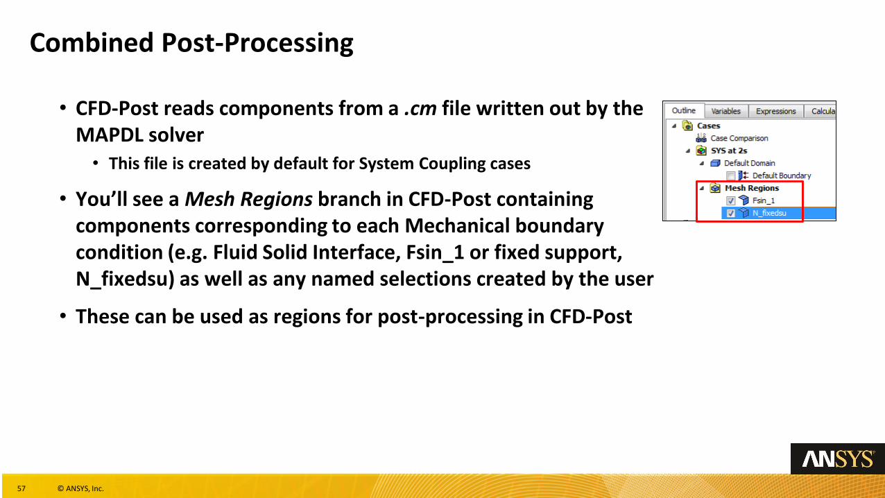
• CFD-Post reads components from a .cm file written out by the MAPDL solver• This file is created by default for System Coupling cases
• You’ll see a Mesh Regions branch in CFD-Post containing components corresponding to each Mechanical boundary condition (e.g. Fluid Solid Interface, Fsin_1 or fixed support, N_fixedsu) as well as any named selections created by the user
• These can be used as regions for post-processing in CFD-Post
58 © ANSYS, Inc.
Summary
• You can launch System Coupling from with Workbench or via RSM and both solvers can run in parallel
• The System Coupling log file provides a Mapping Summary that should always be checked− You can output the interface meshes to csv files and read into CFD-Post to help
diagnose mapping problems
• Restarts can be made from completed runs, interrupted runs and from backup points− When performing restarts review the procedures described earlier, particularly
when making setup changes