Lecture 1Course Explanation and Introduction 2R

Dr. Wim P. KrijnenLecturer Statistics

University of GroningenFaculty of Mathematics and Natural Sciences

Johann Bernoulli Institutefor Mathematics and Computer Science

October 19, 2010

Lecture overview

I Some general remarksI Purpose of the courseI How to do this course?I ECTS, study hours and Mark on course

I General introduction to RI Situations for Using RI InstallingI Help: searching, examples, demonstrations, books,

tutorialsI Reading and writingI Important FunctionsI Some Plots of dataI Some Statistical Tests

I Notes on Chapter 1

Purpose of the course

I Applied statisticsI only little bit of calculusI basic understanding of notation

I Introduction to important statistical conceptsI understanding of concepts such as goodness of fit,

maximum likelihood, applications of central limit theoremI being able to work with several basic distributions and

densitiesI justify choice for statistical test, analyzing data

I Introduction in using RI understanding and programming correct codeI make correct interpretation from outputI make judgement of validity of statistical inference

How to do this course?

I Study the book and presentations wellI learn from examples, exercises, assignments, and trial

examI Print lectures from acrobat (print setup | Lay out | multiple

pages), make notesI Come up with ideas, problems, mistakes, and (sometimes)

frustrations!I Be active and explore!I Ability to write correct R scripts determines usefulness

ECTS, study hours and Mark on course

5 ECT⇒ 5 · 28 = 140 hours of studylectures 4+4 hours during 7 weeks⇒ 56 hoursthere remain 140−56

7 = 12 hours of study per week

M = 0.7 · E + 0.15 ·max (E ,A1) + 0.15 ·max (E ,A2)

M mark of course, E exam, A1 Assignment 1, A2 Assignment 2

> E <- 5; A1 <- 7; A2 <- 7> (M <- 0.7 * E + 0.15 * max(E,A1) + 0.15 * max(E,A2))[1] 5.6> E <- 8; A1 <- 7; A2 <- 7> (M <- 0.7 * E + 0.15 * max(E,A1) + 0.15 * max(E,A2))[1] 8

this holds if and only if E ≥ 5.0if E < 5.0, then M = E (not passing)

General introduction to RSituations for Using R

I Repeated similar problemsI Programming of visualizations: scalable publication ready

plotsI Handle large data setsI Desire flexibility in statistical programmingI Use of modern techniques (bootstrap, robust, Baysian)

Reasons for Using R

I Widely used in statistics and applied sciencesI Reliable free open sourceI incorporated in traditional statistical programs (SPSS,

MINITAB, SAS)I Versatile: Matlab, MySQL, Perl, JAVA, C++, FortranI Numerous libraries with modern methodsI High level language with many built-in-functions (allows

quick programming)

Disadvantages:I Steep learning curve (frequent use helps at lot)I Mainly command line, some Graphical User Interface (GUI)I Use internal C code; pure C++ faster, more efficient

Install R on your personal computer

URL: http://cran.r-project.orgChoose

I operating system: Windows, Linux, MacI base

I html helpType writers to for writing R code

I recommended are Notepad, WinEdt, Kate, emacsI word processors are not recommendedI use syntax highlighting for correct use of symbols {[(

installing libraries

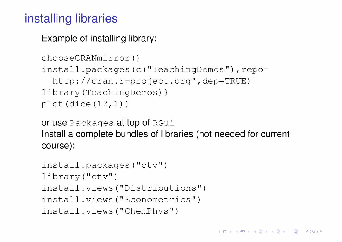
Example of installing library:

chooseCRANmirror()install.packages(c("TeachingDemos"),repo=

http://cran.r-project.org",dep=TRUE)library(TeachingDemos)}plot(dice(12,1))

or use Packages at top of RGuiInstall a complete bundles of libraries (not needed for currentcourse):

install.packages("ctv")library("ctv")install.views("Distributions")install.views("Econometrics")install.views("ChemPhys")

Searching and helpFrom http://cran.r-project.org

I Search, Task Views, Manuals, FAQs, The RJournal, Wiki

I → Contributed: ”R for Beginners”, ”The R Guide”,”Practical Regression and Anova using R”, ”IcebreakeR”,”Notes on the use of R for psychology experiments andquestionnaires”, ”An Introduction to S and The Hmisc andDesign Libraries”

I → Contributed ”R reference card”I Manuals: ”An Introduction to R”, ”The R Language

Definition”, ”Installation and Administration”, ”R DataImport/Export”

Useful tutorial for beginners:http://cran.r-project.org/doc/contrib/Verzani-SimpleR.pdfhttp://www.r-project.org→ choose Books

Help on examples

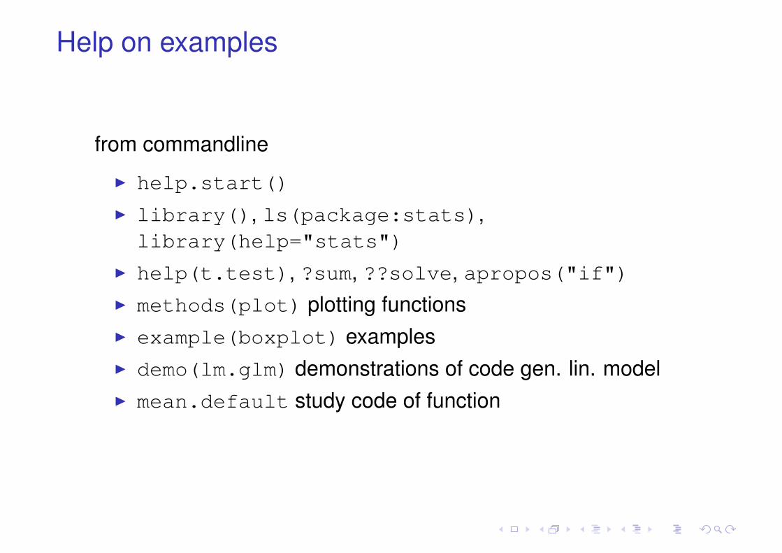
from commandline

I help.start()

I library(), ls(package:stats),library(help="stats")

I help(t.test), ?sum, ??solve, apropos("if")I methods(plot) plotting functionsI example(boxplot) examplesI demo(lm.glm) demonstrations of code gen. lin. modelI mean.default study code of function

Help on Programming

I help(Control) : “for” and “ while” loopsI help(Syntax) : syntax of operatorsI help(Logic) : logical operators AND, OR, negationI help(Arith) : on arithmetic, relational, logical operators,

mathematical functionsI help(Special) : gamma function

Help on Editing: top of GUI Help | Console

Some notes on Chapter 1: R as calculator

illustrating the usual rules for addition, multiplication, etc.

> 2 + 3 * (5+1)[1] 20> ln(10)Error: could not find function "ln"> log(10) # log = ln[1] 2.302585> log10(10)[1] 1> 10ˆ2[1] 100> eˆ1Error: object ’e’ not found> exp(1)[1] 2.718282

Assignment to objects

> x <- 5> x[1] 5> 6 -> z ; z[1] 6> (y <- pi)[1] 3.141593

Executing functions

> x <- 5> print(x) # object x is recognized and printed[1] 5> ls()[1] "x"> rm(list = ls())> ls()character(0)> dir()[1] "Figure1.2.jpg" "Figure12.jpg"[3] "Lecture1.aux" "Lecture1.bbl"

Vectors

> x <- 1:5> x[2][1] 2> x[c(2,4)][1] 2 4> x1 <- seq(1, 5, by = 1)> x2 <- seq(1, 5, length = 5)> x1==x2[1] TRUE TRUE TRUE TRUE TRUE

Mode and ClassSome modes: ”logical”, ”integer”, ”double”, ”complex”, ”raw”,”character”, ”list”, ”expression”, ”name”, ”symbol” and ”function”

> (x <- 1:5)[1] 1 2 3 4 5> mode(x)[1] "numeric"> class(x)[1] "integer"> str(x)int [1:5] 1 2 3 4 5

> (z <- x==3)[1] FALSE FALSE TRUE FALSE FALSE> mode(z)[1] "logical"> as.character(x)[1] "1" "2" "3" "4" "5"> mode(as.character(x))[1] "character"

Vectors

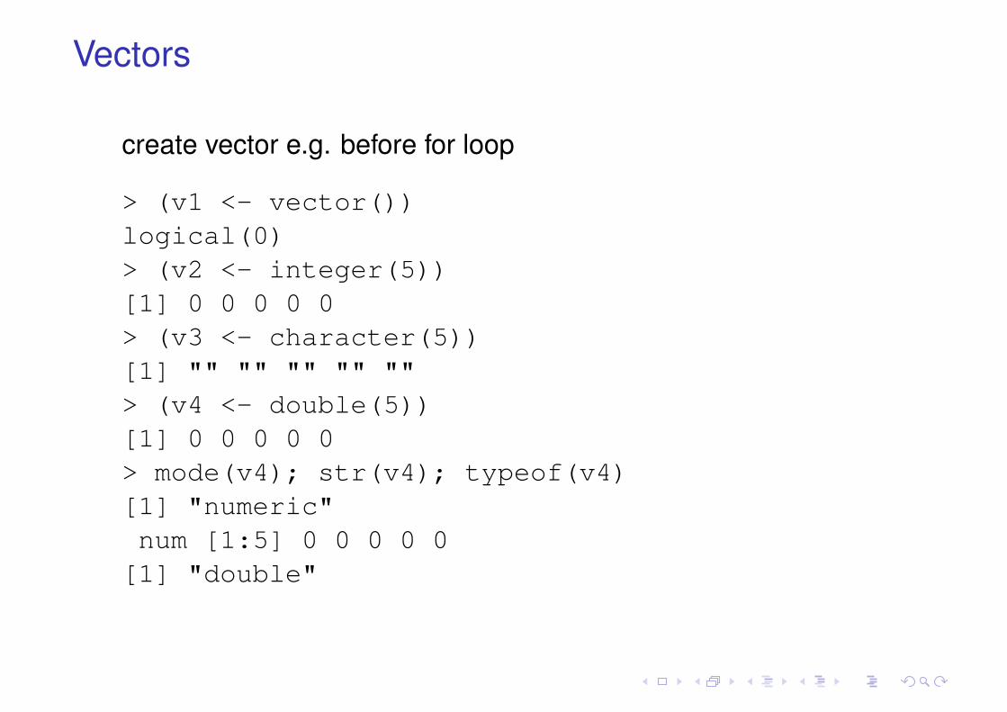
create vector e.g. before for loop

> (v1 <- vector())logical(0)> (v2 <- integer(5))[1] 0 0 0 0 0> (v3 <- character(5))[1] "" "" "" "" ""> (v4 <- double(5))[1] 0 0 0 0 0> mode(v4); str(v4); typeof(v4)[1] "numeric"num [1:5] 0 0 0 0 0

[1] "double"

Functions on vectors

> x <- letters[1:5]> x == c("b")[1] FALSE TRUE FALSE FALSE FALSE> sum(x == c("b"))[1] 1> x <- 1:5> length(x)[1] 5> sum(x)[1] 15> sum(x)/length(x)[1] 3

Arithmetic on vectorsx <- 1:5> x + 1[1] 2 3 4 5 6> x/2[1] 0.5 1.0 1.5 2.0 2.5> x + x[1] 2 4 6 8 10> x[1:4][1] 1 2 3 4> x[1:4] + x[2:5][1] 3 5 7 9> sqrt(x)[1] 1.000000 1.414214 1.732051 2.000000 2.236068> log10(x)[1] 0.0000000 0.3010300 0.4771213 0.6020600 0.6989700> 10ˆlog10(x)[1] 1 2 3 4 5

Dealing with Not Available (NA); indexing> (x <- c(10,20,NA,4,NA,2))[1] 10 20 NA 4 NA 2> mean(x)[1] NA> x[c(1,2,4,6)][1] 10 20 4 2> (i <- is.na(x))[1] FALSE FALSE TRUE FALSE TRUE FALSE> x[i][1] NA NA> !i[1] TRUE TRUE FALSE TRUE FALSE TRUE> x[!i][1] 10 20 4 2> mean(x[!i])[1] 9> mean(x,na.rm = TRUE)[1] 9

Fill vector with random numbers

draw random numbers from uniform distribution

> x <- runif(100000)> round(x[1:5],3)[1] 0.708 0.292 0.123 0.408 0.339> mean(x)[1] 0.4997755> mean(x[x>.5])[1] 0.7499488

Logical operators

> 5 > 4[1] TRUE> 5 >= 4[1] TRUE> 5 == 4[1] FALSE> 5 != 4[1] TRUE> 5 >= 4 & 4 <= 5 # AND[1] TRUE> 5 >= 4 | 4 == 5 # OR[1] TRUE

see also help(Logic)

Some more logic

> x <- sample(c(TRUE,FALSE),5, replace=TRUE,prob=c(1/2,1/2))

> x[1] TRUE FALSE FALSE FALSE TRUE> is.logical(x); is.numeric(x); is.integer(x);[1] TRUE[1] FALSE[1] FALSE> sum(x); sum(as.integer(x))[1] 2[1] 2

Conditional executionif (test) {execute some} else {execute some else}> bmi <- 22> goodhealth <- logical()> if (bmi<25) {goodhealth <- TRUE} else {+ goodhealth <- FALSE}> goodhealth[1] TRUE> bmi <- c(22,28,35,19) # bmi of 5 persons> goodhealth <- logical(length(mbi))> for (i in 1:length(bmi)) if (bmi[i] < 25)+ {goodhealth[i] <- TRUE} else {+ goodhealth[i] <- FALSE}> goodhealth[1] TRUE FALSE FALSE TRUE> rm(goodhealth)> ifelse(bmi<25, goodhealth <- TRUE,+ goodhealth <- FALSE)[1] TRUE FALSE FALSE TRUE

Paste

> x <- letters[1:5]> paste(x[1],313:317,sep=’-bla-’)[1] "a-bla-313" "a-bla-314" "a-bla-315" "a-bla-316"

"a-bla-317"> paste("AY34X",seq(313,317,by=2),sep = "")[1] "AY34X313" "AY34X315" "AY34X317"paste("Today is", date())a <- dir()

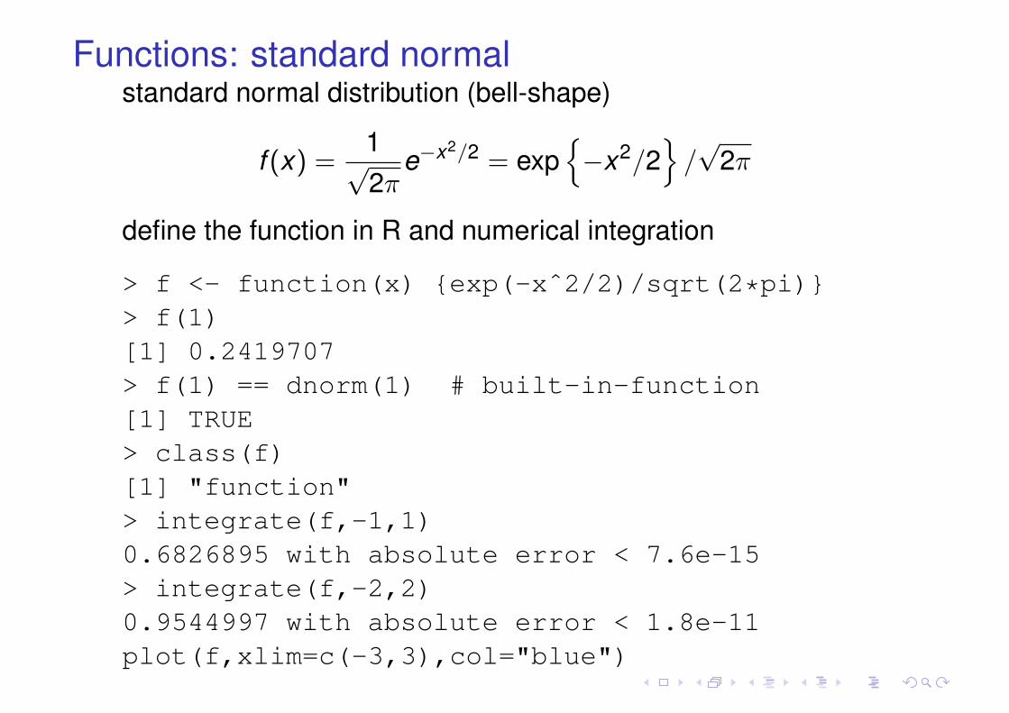
Functions: standard normalstandard normal distribution (bell-shape)

f (x) =1√2π

e−x2/2 = exp{−x2/2

}/√

2π

define the function in R and numerical integration

> f <- function(x) {exp(-xˆ2/2)/sqrt(2*pi)}> f(1)[1] 0.2419707> f(1) == dnorm(1) # built-in-function[1] TRUE> class(f)[1] "function"> integrate(f,-1,1)0.6826895 with absolute error < 7.6e-15> integrate(f,-2,2)0.9544997 with absolute error < 1.8e-11plot(f,xlim=c(-3,3),col="blue")

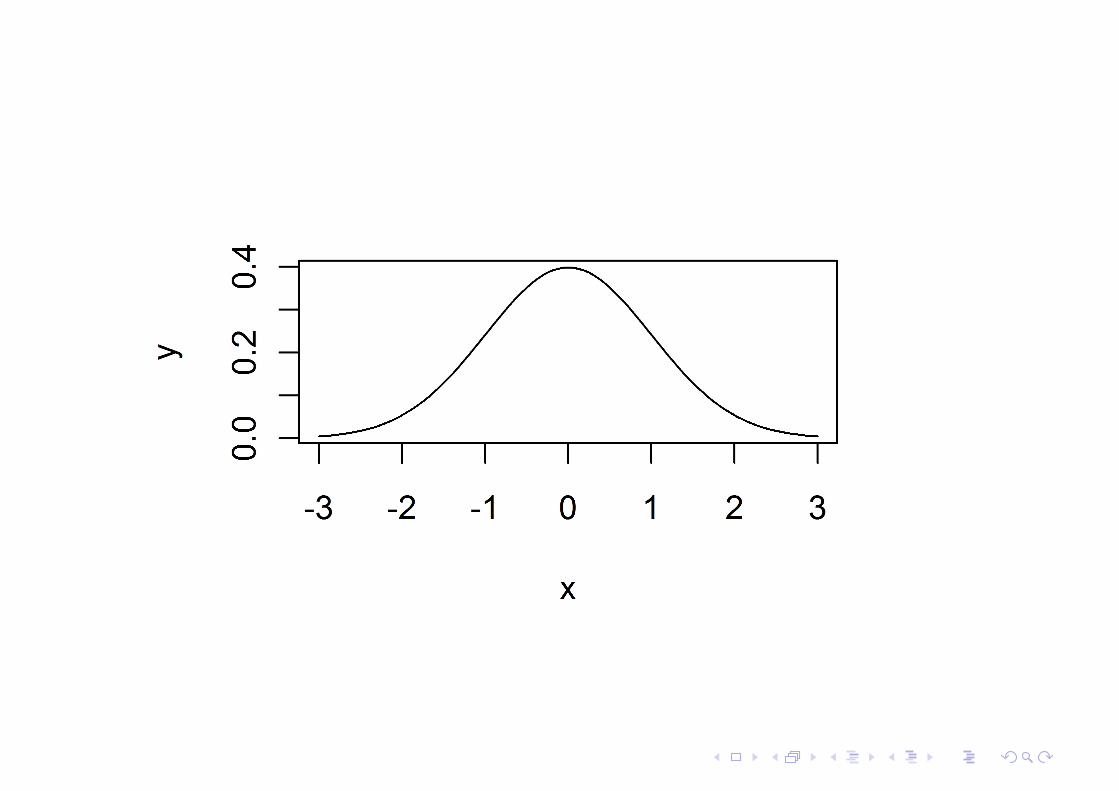
bell shaped normal density function f (x) = e−x2/2/√

2π

running code from a file

Use your favorite type writer to save the code

setwd("C:/work/StatisticsForAINF/book/ch1")x <- seq(-3, 3, length = 101)y <- dnorm(x)plot(x, y, type = ’l’)

in a file called e.g. "acodechunckinR.R"use dir() to verify that your file is in de working directoryin the R console type

source("acodechunckinR.R")

to run the code

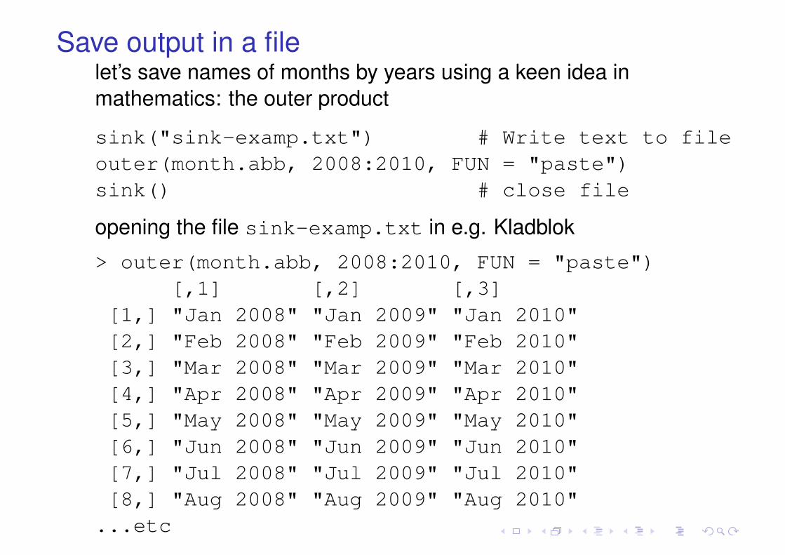
Save output in a filelet’s save names of months by years using a keen idea inmathematics: the outer product

sink("sink-examp.txt") # Write text to fileouter(month.abb, 2008:2010, FUN = "paste")sink() # close file

opening the file sink-examp.txt in e.g. Kladblok

> outer(month.abb, 2008:2010, FUN = "paste")[,1] [,2] [,3]

[1,] "Jan 2008" "Jan 2009" "Jan 2010"[2,] "Feb 2008" "Feb 2009" "Feb 2010"[3,] "Mar 2008" "Mar 2009" "Mar 2010"[4,] "Apr 2008" "Apr 2009" "Apr 2010"[5,] "May 2008" "May 2009" "May 2010"[6,] "Jun 2008" "Jun 2009" "Jun 2010"[7,] "Jul 2008" "Jul 2009" "Jul 2010"[8,] "Aug 2008" "Aug 2009" "Aug 2010"

...etc

Brief overview of important functions

Some basic R functionsR function purposerm(list=ls()) remove objectsq() quithistory() list of previous input linesls(),objects() list of loaded objectsgetwd,setwd getting, setting working directorydir() list of file names working directoryfunction define real to real functionsample simulated discrete samplingrunif random sampling from uniform distributiongrep,regexpr regular expressions

Warning on some functions used throughout the book

End of Chapter 1 there are functions defined to save space inthe book openg, saveg, h, ndq

I need to be defined before usageI these are not “very spectacular”

You should now be able to do assignments of chapter 1