Embed Size (px)
DESCRIPTION
Tree-based methods, neutral networks. Lecture 10. Tree-based methods. Statistical methods in which the input space (feature space) is partitioned into a set of cuboids (rectangles), and then a simple model is set up in each one. Why decision trees. Compact representation of data - PowerPoint PPT Presentation
Citation preview

Lecture 10

Tree-based methods
Statistical methods in which the input space (feature space) is partitioned into a set of cuboids (rectangles), and then a simple model is set up in each one

Why decision trees
Compact representation of dataPossibility to predict outcome of new
observations

Tree structureRootNodesLeaves (terminal nodes)Parent-child relationshipConditionLabel is assigned to a leaf
N4 N5 N6 N7
Cond.1
Cond.3
Cond.2
Cond.4 Cond.5 Cond.6

Example
Non-mammals
Warm
Leaf nodes
Body temperature?
Gives birth?
Non-mammals
Mammals
Cold
NoYes
Internal node
Root node

How to build a decision tree: Hunt’s algorithm
Proc Hunt(Dt,t)
Given Data set Dt={(X1i,..Xpi, Yi), i=1..n}, t-curr.node
If all Yi are equal mark t as leaf with label Yi
If not, use the test condition to split into Dt1…Dtn, create children t1…tn and run Hunt(Dt1,t1),…, Hunt(Dtn,tn)

Hunt’s algorithm example
0
10
20
10 20
X1
X2 X2
0 1 X11
01
<9 >=9
<16 <7>=16 >=7
<15 >=15
}),{(),(ˆ21
121 m
N
mm RXXIcXXf

Hunt’s algorithmWhat if some combinations of attributes are missing?
Empty nodeIs assigned the label representing the majority class among the records (instances, objects, cases) in its parent node.
All records in a node have identical attributesThe node is declared a leaf node with the same class label as the majority class of this node

CART: Classification and regression treesRegression treesGiven Dt={(X1i,..Xpi, Yi), i=1..n}, Y –
continuous, build a tree that will fit the data best
Classification treesGiven Dt={(X1i,..Xpi, Yi), i=1..n}, Y –
categorical, build a tree that will classify the observations best

A CART algorithm: Regression trees
Splitting variables and split points
Consider a splitting variable j and a split point s, and define the pair of half planes
We seek the splitting variable j and split point s that solve
}|{),( and}|{),( 21 sxxsjRsxxsjR jj
),( ),(
22
21,
1 2
21)(min)(minmin
sjRx sjRxicicsj
i i
cycy
Aim:Want to find ; computationally expensive to
test all possible splits. Instead
iii fy 2min

Post-pruningHow large tree to grow? Too large – overfitting!
Grow a large tree T0
Then prune this tree using post-pruning
Define a subtree T and index its terminal nodes by m, with node m representing region Rm.
Let |T| denote the number of terminal nodes in T and set
where
Then minimize this expression, using cross-validation to select the factor that penalizes complex trees.
mi Rx
im
m yN
c1
ˆ
||)ˆ()(||
1
2 TcyTCT
m Rxmi
mi

CART: Classification treesFor each node define proportions
Define measure of impurity
s
iik kyI
sp
1
1
i
c
ii
c
iii
p
p
pp
max1errortion Classifica
)(1Gini
)(logEntropy
1
0
2
1
02
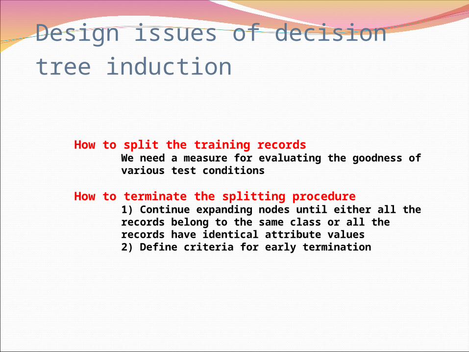
Design issues of decision tree induction
How to split the training recordsWe need a measure for evaluating the goodness of various test conditions
How to terminate the splitting procedure1) Continue expanding nodes until either all the records belong to the same class or all the records have identical attribute values2) Define criteria for early termination

How to split: CARTSelect splitting with max information gain
where I(.) is the impurity measure of a given node, N is the total number of records at the parent node, and N(vj) is the is the number of records associated with the child node vj
k
jj
j vIN
vNparentI
1
)()(
)(

How to split: C4.5
Impurity measures such as Gini index tend to favour attributes that have a large number of distinct values
Strategy 1: Restrict the test conditions to binary splits only
Strategy 2: Use the gain ratio as splitting criterion
k
jjj
k
jj
j
vpvp
vIN
vNparentI
12
1
info
)(log)(
)()(
)(
infoSplit ratioGain

Constructing decision trees
Yes
Home owner
Married
Defaulted
= No
Defaulted
= No
Marital status
Defaulted = ?
Not married
NoHome owner
Marital status
Annual income
Defaulted borrower
No Divorced 95K YesNo Married 100K NoNo Married 60K NoNo Married 75K NoNo Single 70K NoNo Single 85K YesNo Single 90K YesYes Divorced 220K NoYes Married 120K NoYes Single 125K No
Income
> 100 K≤ 100 K

Expressing attribute test conditions
Binary attributesBinary splits
Nominal attributesBinary or multiway splits
Ordinal attributesBinary or multiway splits honoring the order of the attributes
Continuous attributesBinary or multiway splits into disjoint interval

Characteristics of decision tree induction
Nonparametric approach (no underlying probability model)
Computationally inexpensive techniques have been dveloped for constructing decision trees. Once a decision tree has been built, classification is extremely fast
The presence of redundant attributes will not adversely affect the accuracy of decision trees
The presence of irrelevant attributes can lower the accuracy of decision trees, especially if no measures are taken to avoid overfitting
At the leaf nodes, the number of records may be too small (data fragmentation)

Neural networks
Joint theoretical framework for prediction and classification

Principal components regression (PCR)
Extract principal components (transformation of the inputs) as derived features, and then model the target (response) as a linear function of these features
MmZ Tmm ,...,1, Xα
x1 x2 xp
z1 z2 zM…
…
y
ZβTy 0

Extract linear combinations
of the inputs as derived features, and then model the target (response) as a linear function of a sigmoid function of these features
MmZ Tmmm ,...,1,)( 0 Xα
x1 x1 xp
z1 z2 zM…
…
y
ZβTy 0
MmTmm ,...,1,0 Xα
Neural networks with a single target

Artificial neural networksIntroduction from biology:NeuronsAxonsDendritesSynapseCapabilities of neural networks:Memorization (noise stable, fragmentary
stable!)Classification
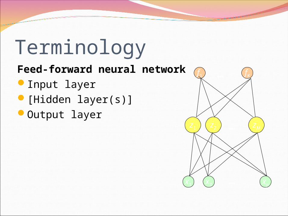
TerminologyFeed-forward neural networkInput layer[Hidden layer(s)]Output layer
x1 x2 xp
z1 z2 zM…
…
f1 fK…

TerminologyFeed-forward network
Nodes in one layer are connected to the nodes in next layer
Recurrent networkNodes in one layer may be connected to the
ones in previous layer or within the same layer

TerminologyFormulas for multilayer perceptron (MLP)
C1, C2 combination functiong, ς activation functionα0m β0k bias of hidden unit
αim βjk weight of connection
MmZC
Tmmm ,...,1,)(
1
0 Xα
KkgfC
Tkkk ,...,1,)(
2
0 Z

Recommended readingBook, paragraph 9.2EM Reference: Tree Node
Start with:Book, paragraph 11EM Reference: Neural Network node