Embed Size (px)
Citation preview

Lecture 10
Chapter 7: Species Interactions/Competition
Chapter 8: Mutualisms

Terminology • -/- Competition
• -/+ Predation and other associations where one species benefits and the other is harmed
• +/0 Commensalism
• +/+ Mutualism
• Facultative
• Obligatory
• Carnivorous predators
• Parasitoids
• Parasitism:
– Ectoparasites
– Endoparasites
• Herbivores
• Seed predation

7.1: Concept of Niche
• Joseph Grinnell (1917)
• Charles Elton (1927)
• G. E. Hutchinson (1957)
• Robert Ricklefs (1997)
• Informal and Formal definitions
• Fundamental Niche =
• Realized Niche =
Please read about these researchers on your own
7.2: History of Interspecific competition
• Tansley (1917) : context dependent competitive exclusion, Plant Ex.
• Galium saxitale
• Galium sylvestre

7.2: History of Interspecific competition
Gause (1934) The struggle for existence, Animal Ex.
– Yeast
– Protozoans, Paramecium caudatum and P. aurelia
– Fig. 7.1 in text and original (Chapter 5: Fig. 21) shown here:

Gause’s results (1934)
Competitive Exclusion Principle:
• No two species can occupy the same ecological niche
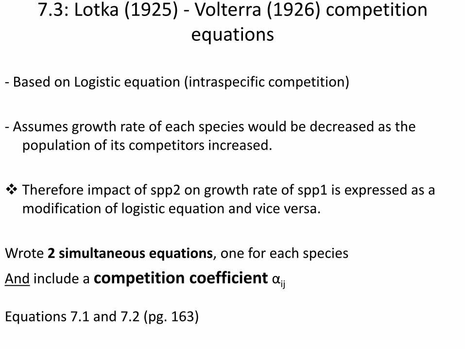
7.3: Lotka (1925) - Volterra (1926) competition equations
- Based on Logistic equation (intraspecific competition)
- Assumes growth rate of each species would be decreased as the population of its competitors increased.
Therefore impact of spp2 on growth rate of spp1 is expressed as a modification of logistic equation and vice versa.
Wrote 2 simultaneous equations, one for each species
And include a competition coefficient αij
Equations 7.1 and 7.2 (pg. 163)

7.3: Lotka (1925) - Volterra (1926) competition equations
Equation 7.1 dN1/dt = r1N1[K1-N1-α12N2/K1]
Equation 7.2 dN2/dt = r2N2[K2-N2-α21N1/K2]
Where:
N1, N2 = number of individuals per species
r1, r2 = intrinsic rate of each species
K1, K2 = carrying capacity of each species
α1 2 = competition coefficient – effect of species 2 on species 1
α21 = competition coefficient – effect of species 1 on species 2
t = time
(pg. 163)

Competition Coefficient Competition Coefficient: αij
• Value normally ranges between 0 and 1
• If = 0, indicates no competition between two species. No reason to pursue further since no competition.
• If coefficient is negative, then each species benefits growth of one another, ~ mutualistic interaction
• If = 1, indicates intraspecific competition
Thus interspecific competition is usually less intense than intraspecific competition and is noted by 0> α <1 value
• Lots of parameters to estimate (r, K, α ) but can simplify with:
“Equilibrium Analysis” – equate popln growth to zero, AFTER RESULTS of competition completed: dN1/dt = 0 and dN2/dt = 0

Lotka-Volterra cont.
Popln of species 1
Pop
ln o
f sp
ecie
s 2
Zero isocline for pop 1
(0,K1/α12)
(K1,0)
N2 = (K1-N1)/α12
See also: Fig. 7.3 Zero isocline for species 2
Fig. 7.2
Competition coefficients determined by ratio of two species carrying capacities α12 = K1/K2 (eq: 7.10)

Lotka-Volterra cont.
Competition coefficients determined by ratio of 2 species K
Recall: α12 = K1/K2 (eq: 7.10)
By placing zero isoclines (Saturation levels) on same graph 4 combo’s possible:
1) Fig. 7.4 Species 1 wins (pg. 167) K1/α12>K2 with K1>K2/α21
2) Fig. 7.5 Species 2 wins (pg. 167) K2>K1/α12 with K2/α21>K1
3) Fig. 7.6 Unstable equilibrium (S) or competitive exclusion with indefinite winner (pg. 168) K1>K2/α21 with K2>K1/α12
4) Fig. 7.7 Coexistence of both species at stable equilibrium, E (pg. 168)
K1/α12>K2 with K2/α21>K1

7.4: Laboratory competition experiments
Table 7.1 Thomas Parks (1954) Flour beetles pg 169
Temp % Rel .Humidity
Climate T confusum T castaneum
34 70 Hot-moist 0 100
34 30 Hot-dry 90 10
29 70 Warm-moist 14 86
29 30 Warm-dry 87 13
24 70 Cold-moist 71 29
24 30 Cold-dry 100 0

7.5 Resource-based competition theory
Fig. 7.8 Per capita growth as a function of resource availability (Pg 171)
• Fig. 7.9 Per capita growth as a fn of resource availability, BUT with constant mortality. (Pg 172)
• R* = dN/dt = 0: amt of resource producing a per capita growth rate equals zero, thus R* growth rate balances death.
• KRi = supply rate
• Ri = resource quantity
• q = consume resource at rate q
• b = efficiency individual converts resources to new individuals.
• dRi/dt = kRi (Eq. 7.11)
• In form of logistic equation: dN/dt = bkRiN(1-qN/kRi) (Eq. 7.13)
• Fig. 7.10 Popln size and resource dynamics (Pg 172)
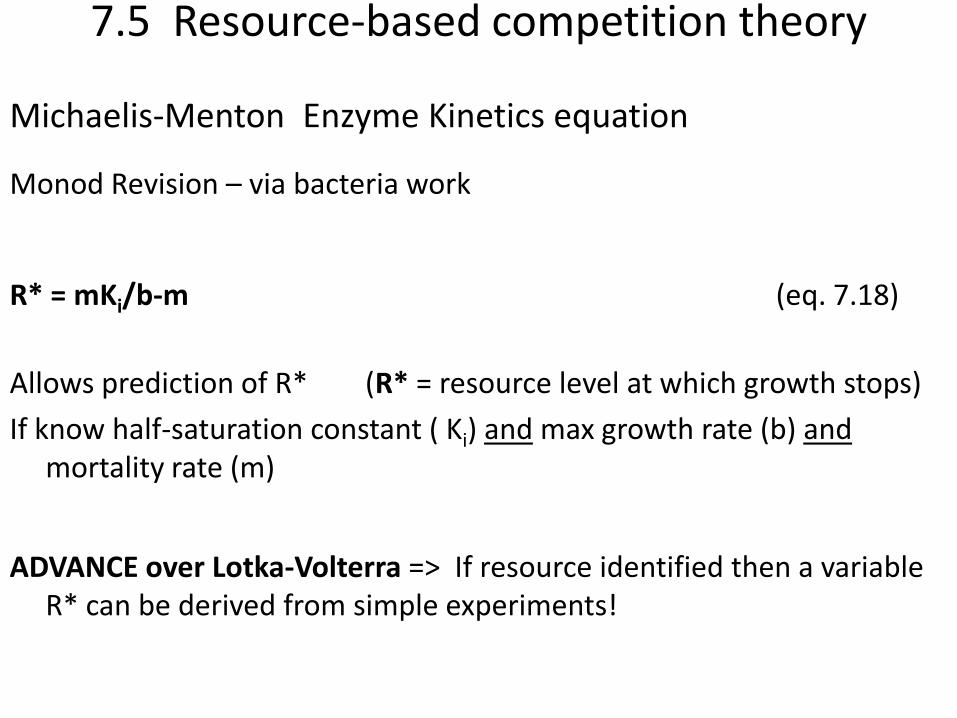
7.5 Resource-based competition theory
Michaelis-Menton Enzyme Kinetics equation
Monod Revision – via bacteria work
R* = mKi/b-m (eq. 7.18)
Allows prediction of R* (R* = resource level at which growth stops)
If know half-saturation constant ( Ki) and max growth rate (b) and mortality rate (m)
ADVANCE over Lotka-Volterra => If resource identified then a variable R* can be derived from simple experiments!

7.5 Resource-based competition theory
R* Rule = for any given resource (R),
if determine R* value for each species grown alone in same environment,
then species w/ lowest R* should competitively exclude all other species when grown together given enough time in same constant environment .
NOT Predicted by Lotka-Volterra: A species w/high affinity for a resource can still LOSE if it has a low growth rate (r) & high death (m).
See Table 7.2 R* Rule calculations R* < R0 or all species die out because of lack of resources

7.6 Spatial competition and the competition-colonization trade off
Multiple species can coexist within a community without resulting into one species yielding to the other – idea is foundation of competition-colonization trade-off idea 1st proposed by Levins and Culver (1971)
dP/dt = cP(1-P)- εP (Eq. 7.21)
P = 1- (ε/c) (Eq. 7.22)
c = ε/ (1- P) (Eq. 7.23)
c1 > ε1 Eq. 7.29a
c2> c1(c1 + ε2 - ε1 )/ ε1 Eq. 7.29b
Spatial competition hypothesis: generalized for multiple species interactions. Proposes stable coexistence for inferior competitors in a diverse community.

7.7 Evidence for competition in nature – Read on your own please
• Connell’s barnacles
• Ant succession:
opportunists
extirpators
insinuators
• Literature Review of field studies of competition

7.8 Indirect Evidence for competition & natural experiments - Read on your own please
• Ghost of Competition Past
Jared Diamond (1983) & 3 advantages of natural experiments
1) Gather data quickly
2) Assess situations where experimental manipulation is unlikely
3) Allows assessment of long term ecological and evolutionary pressures’ end result
7.8 Indirect Evidence for competition & natural experiments – Read on your own please
Five types of indirect evidence from natural experiments:
Jared Diamond (1983) & 3 advantages of natural experiments
1) Ecological release
2) Contiguous allopatry
3) Niche partitioning
4) Character displacement
5) Historical replacement

Chap. 7: Highlights – Competition
• The ecological niche
• The competitive exclusion principle
• The Lotka–Volterra competition equations
• Resource-based competition theory
• Spatial competition and the competition–colonization trade-off
• Evidence for competition from nature
• Indirect evidence for competition and “natural experiments”

Mutualisms: Chapter 8

8.1 Mutualism or Parasitism
• +/+ Mutualism
• +/- Parasitism
• Facultative
• Obligatory
• Mutualism are complex and do not often fit into a neat category of facultative or obligatory
• May be context dependent and exist only under a unique set of conditions
• Some mutualisms more common in tropical vs. temperate regions
• Examples?

Ant – Acacia mutualisms

Obligate Mutualisms - Yucca and Yucca moth
http://4.bp.blogspot.com/-MKwV9eV7G-A/TdZsCDd3TcI/AAAAAAAAAEM/4Hg5PSXiyp4/s1600/Yucca%2Bfilamentosa.jpg
http://www.fs.fed.us/wildflowers/pollinators/pollinator-of-the-month/images/yuccamoth/yucca_moth2_Alan_Cressler_lg.jpg

Fig – Fig wasp obligate mutualism
http://4.bp.blogspot.com/-6HiPlL4rzqw/Tp9a3DFu6UI/AAAAAAAAAD4/9-MS1JLAYug/s1600/Fig%2BWasp%2BCycle.jpg

8.2: Modeling mutualism
Back to the Lotka-Volterra equation
• “orgy of mutual benefaction” (Robert May 1981)
• Mutualism coefficients, c1 and c2 , replace competition coefficients
c1 = measures rate an indiv. of N2 benefits from growth rate of N1
c2 = measure rate an indiv. of N1 benefits from growth rate of N2
dN1/dt = r1N1 [K1 + c1N2-N1]/K1 Eq. 8.1, pg 191
dN2/dt = r2N2 [K2 + c2N1-N2]/K2 Eq. 8.2, pg 191

8.2: Modeling mutualism
dN1/dt = r1N1 [K1 + c1N2-N1]/K1 Eq. 8.1
dN2/dt = r2N2 [K2 + c2N1-N2]/K2 Eq. 8.2
Perform “equilibrium analysis” by setting dN1 and dN2 to zero
Results in the population of each species being increased beyond its carrying capacity w/ additional individuals of its partner species.
The more intense the mutualism, (>er benefits to partner spp.) the larger the equilibrium popln becomes:
N1 = K1 + c1N2 Eq. 8.3
N2 = K2 + c2N1 Eq. 8.4
See pg. 191

8.2: Modeling mutualism
N1 = K1 + c1N2 Eq. 8.3
N2 = K2 + c2N1 Eq. 8.4
The interaction is stable when only one partner benefits from the interaction.
If c2 = 0, then N2 cannot exceed K2 and N1 stabilizes at K1 + c1K2
Another approach: substitute carrying capacity after mutualism & note as K*1 and K*2
Eq. 8.5 K*1 = K1 + c1N2 Recall: c = mutualism coefficient
Eq. 8.6 K*2 = K2 + c2N1
Eq. 8.7 dN1/dt = r1N1[K*1 -N1/ K*1] = r1N1[K1 + c1N2-N1/K1+c1N2]
Eq. 8.8 dN2/dt = r2N2[K*2 -N2/ K*2] = r2N2[K2 + c2N1-N2/K2+c2N1]

8.2: Modeling mutualism Lotka-Volterra approach is phenomenological in design
Mechanistic approach needed: Based on actual rates of exchange of relevant resources between 2 mutualisms
Since each interaction is unique, complex, and context dependent, model generalizations are hard to arrive at that have any meaning.
No standard approach to modeling mutualism
Assess the following points:
1) Mutualism involve costs and benefits
2) Costs set limits on evolution of mutualism
3) Conflict of interest exists between mutualists
4) Organisms that cheat – often receive the benefits
5) Related or similar organisms may benefit by acting as parasites
6) Mutualisms may evolve toward parasitism
7) Continuous coevolution is needed to maintain mutualism

Chap 8: Highlights – Mutualisms
• Mutualism or parasitism?
• Modeling mutualism
• The costs of mutualism