Lecture 10 Page 1 CS 239, Spring 2007 Experiment Designs for Categorical Parameters CS 239 Experimental Methodologies for System Software Peter Reiher

Lecture 10Page 1CS 239, Spring 2007

Experiment Designs for Categorical Parameters

CS 239Experimental Methodologies for

System SoftwarePeter Reiher

May 10, 2007


Outline

• Categorical parameters

• One factor designs

• Two factor full factorial designs


Categorical Parameters

• Some experimental parameters don’t represent a range of values

• They represent discrete alternatives

• With no necessary relationship between alternatives


Examples of Categorical Variables

• Different processors

• Different compilers

• Different operating systems

• Different denial of service defenses

• Different applications

• On/off settings for configurations


Why Different Treatment?

• Most models we’ve discussed imply there is a continuum of parameter values

• Essentially, they’re dials you can set to any value

• You test a few, and the model tells you what to expect at other settings


The Difference With Categorical Parameters

• Each is a discrete entity

• There is no relationship between the different members of the category

• There is no “in between” value

– Models that suggest there are can be deceptive


Basic Differences in Categorical Models

• Need separate effects for each element in a category– Rather than one effect multiplied times the

parameter’s value• No claim for predictive value of model

– Used to analyze differences in alternatives• Slightly different methods of computing effects

– Most other analysis techniques are similar to what we’ve seen elsewhere


One Factor Experiments

• If there’s only one important categorical factor

• But it has more than two interesting alternative– Methods work for two alternatives, but

they reduce to 21 factorial designs• If the single variable isn’t categorical,

examine regression, instead• Method allows multiple replications


What is This Good For?

• Comparing truly comparable options

– Evaluating a single workload on multiple machines

– Or with different options for a single component

– Or single suite of programs applied to different compilers


What Isn’t This Good For?

• Incomparable “factors”

– Such as measuring vastly different workloads on a single system

• Numerical factors

– Because it won’t predict any untested levels


An Example One Factor Experiment

• You are buying VPN server to encrypt/decrypt all external messages– Everything padded to single msg size, for

security purposes• Four different servers are available• Performance is measured in response time

– Lower is better• This choice could be assisted by a one-

factor experiment


The Single Factor Model

• yij = j + eij

• yij is the ith response with factor at alternative j

• is the mean response

• j is the effect of alternative j

• eij is the error term j 0


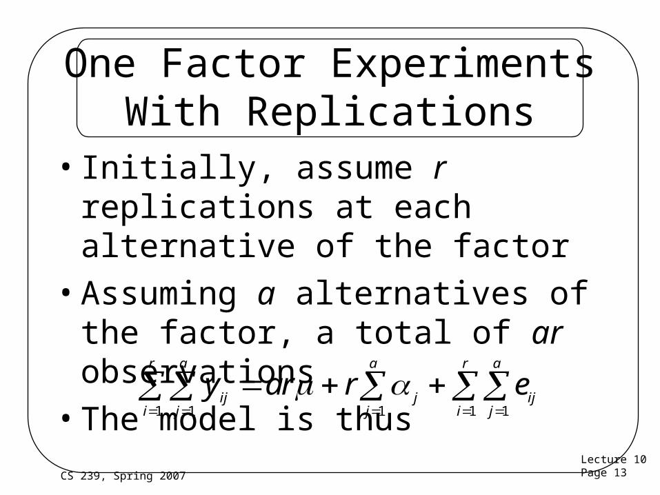
One Factor Experiments With Replications

• Initially, assume r replications at each alternative of the factor

• Assuming a alternatives of the factor, a total of ar observations

• The model is thusy ar r e

ijj

a

i

r

jj

a

ijj

a

i

r

11 1 11


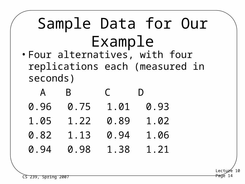
Sample Data for Our Example

• Four alternatives, with four replications each (measured in seconds)

A B C D

0.96 0.75 1.01 0.93

1.05 1.22 0.89 1.02

0.82 1.13 0.94 1.06

0.94 0.98 1.38 1.21


Computing Effects

• We need to figure out and j

• We have the various yij’s

• So how to solve the equation?

• Well, the errors should add to zero

• And the effects should add to zero

eij

j

a

i

r

11

0

j

j

a

0

1


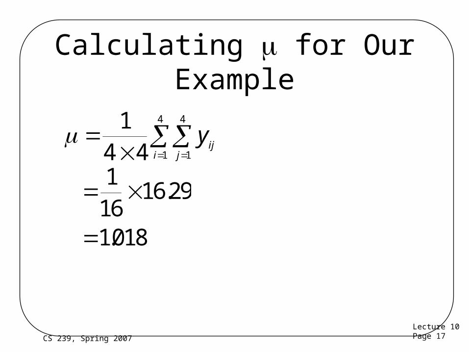
Calculating

• Since sum of errors and sum of effects are zero,

• And thus, is equal to the grand mean of all responses

y arij

j

a

i

r

11

0 0

111ar

y yij

j

a

i

r

..


Calculating for Our Example

14 4 1

4

1

4

yij

ji

116

16 29

1018

.

.


Calculating j

• j is a vector of responses

– One for each alternative of the factor

• To find the vector, find the column means

• For each j, of course

• We can calculate these directly from observations

yr

yj ij

i

r

.

11


Calculating a Column Mean

• But we also know that yij is defined to be

• So,

y eij j ij

11r

r r ej ij

i

r

yr

ej j ij

i

r

.

11


Calculating the Parameters

• Remember, the sum of the errors for any given row is zero, so

• So we can solve for j -

yr

r rj j. 1

0

j

j j j

y y y . . ..


Parameters for Our Example

Server A B C DColumnMean .9425 1.02 1.055 1.055

Subtract (1.018) from column means to get parameters

Parameters

-.076 .002 .037 .037


Estimating Experimental Errors

• Estimated response is

• But we measured actual responses

– Multiple ones per alternative

• So we can estimate the amount of error in the estimated response

• Using methods similar to those used in other types of experiment designs

y j j


Finding Sum of Squared Errors

• SSE estimates the variance of the errors

• We can calculate SSE directly from the model and observations

• Or indirectly from its relationship to other error terms

SSE eijj

a

i

r

2

11


SSE for Our Example

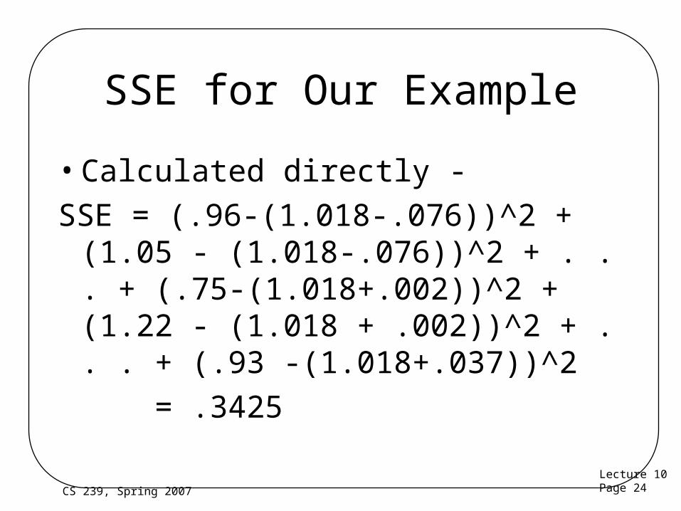
• Calculated directly -

SSE = (.96-(1.018-.076))^2 + (1.05 - (1.018-.076))^2 + . . . + (.75-(1.018+.002))^2 + (1.22 - (1.018 + .002))^2 + . . . + (.93 -(1.018+.037))^2

= .3425


Allocating Variation• To allocate variation for this model, start by

squaring both sides of the model equation

• Cross product terms add up to zero

– Why?

y e e eij j ij j ij j ij2 2 2 2 2 2 2

y e

cross products

iji j i j

ji j

iji j

2 2 2 2

, , , ,


Variation In Sum of Squares Terms

• SSY=SS0+SSA+SSE

• Giving us another way to calculate SSE

SSY yiji j

2

,

SS arj

a

i

r0 2

11

2

SSA rjj

a

i

r

jj

a

2

11

2

1


Sum of Squares Terms for Our Example

• SSY = 16.9615

• SS0 = 16.58256

• SSA = .03377

• So SSE must equal 16.9615-16.58256-.03377

– Which is .3425

– Matching our earlier SSE calculation


Assigning Variation• SST is the total variation

• SST = SSY - SS0 = SSA + SSE

• Part of the total variation comes from our model

• Part of the total variation comes from experimental errors

• A good model explains a lot of variation


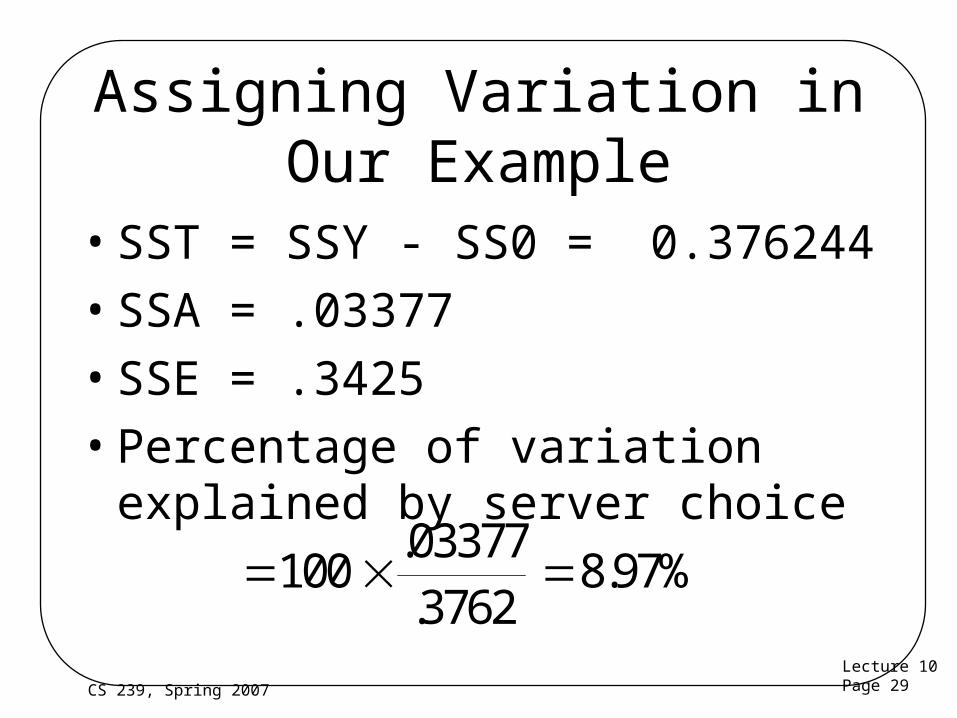
Assigning Variation in Our Example

• SST = SSY - SS0 = 0.376244

• SSA = .03377

• SSE = .3425

• Percentage of variation explained by server choice

10003377

37628 97%

.

..


Analysis of Variance

• The percentage of variation explained can be large or small

• Regardless of which, it may be statistically significant or insignificant

• To determine significance, use an ANOVA procedure – Assumes normally distributed errors . . .


Running an ANOVA Procedure• Easiest to set up a tabular method

• Like method used in regression models

– With slight differences

• Basically, determine ratio of the Mean Squared of A (the parameters) to the Mean Squared Errors

• Then check against F-table value for number of degrees of freedom


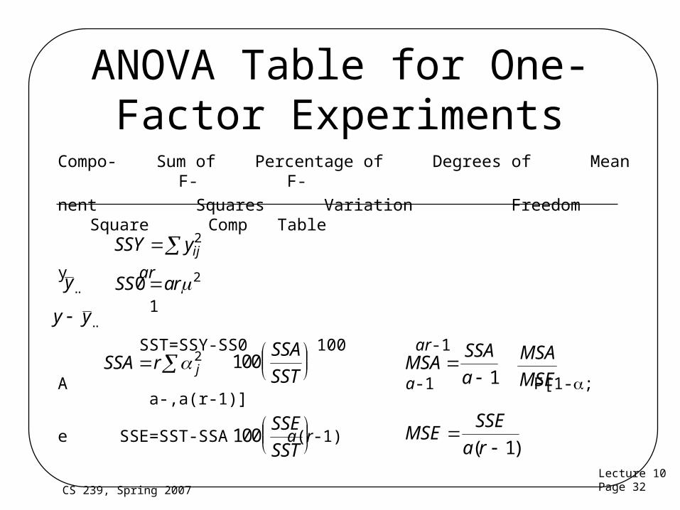
ANOVA Table for One-Factor Experiments

Compo- Sum of Percentage of Degrees of Mean F- F-

nent Squares Variation Freedom Square Comp Table

y ar

1

SST=SSY-SS0 100 ar-1

A a-1 F[1-; a-,a(r-

1)]

e SSE=SST-SSA a(r-1)

SSY yij 2

y.. SS ar0 2

y y ..

SSA r j 2 MSASSA

a

1MSA

MSE

100SSE

SST

MSESSE

a r

( )1

100SSA

SST


ANOVA Procedure for Our Example

Compo- Sum of Percentage of Degrees of Mean F- F-

nent Squares Variation Freedom Square Comp Table

y 16.96 16

16.58 1

.376 100 15

A .034 8.97 3 .011 .394 2.61

e .342 91.0 12 .028

y..

y y ..


Analysis of Our Example ANOVA

• Done at 90% level

• Since F-computed is .394, and the table entry at the 90% level with n=3 and m=12 is 2.61,

– The servers are not significantly different


One-Factor Experiment Assumptions

• Analysis of one-factor experiments makes the usual assumptions– Effects of factor are additive– Errors are additive– Errors are independent of factor alternative– Errors are normally distributed– Errors have same variance at all alternatives

• How do we tell if these are correct?


Visual Diagnostic Tests

• Similar to the ones done before

– Residuals vs. predicted response

– Normal quantile-quantile plot

– Perhaps residuals vs. experiment number


Residuals vs. Predicted For Our Example

-0.3

-0.2

-0.1

0

0.1

0.2

0.3

0.4

0.9 0.95 1 1.05 1.1


Residuals vs. Predicted, Slightly Revised

-0.3

-0.2

-0.1

0

0.1

0.2

0.3

0.4

0.9 0.95 1 1.05 1.1


What Does This Plot Tell Us?• This analysis assumed the size of the errors was

unrelated to the factor alternatives• The plot tells us something entirely different

– Vastly different spread of residuals for different factors

• For this reason, one factor analysis is not appropriate for this data– Compare individual alternatives, instead– Using methods discussed earlier


Could We Have Figured This Out Sooner?

• Yes!

• Look at the original data

• Look at the calculated parameters

• The model says C & D are identical

• Even cursory examination of the data suggests otherwise


Looking Back at the Data

A B C D

0.96 0.75 1.01 0.93

1.05 1.22 0.89 1.02

0.82 1.13 0.94 1.06

0.94 0.98 1.38 1.21

Parameters

-.076 .002 .037 .037


Quantile-Quantile Plot for Example

-0.4

-0.3

-0.2

-0.1

0

0.1

0.2

0.3

0.4

-2.5 -2 -1.5 -1 -0.5 0 0.5 1 1.5 2 2.5


What Does This Plot Tell Us?

• Overall, the errors are normally distributed

• If we only did the quantile-quantile plot, we’d think everything was fine

• The lesson - test all the assumptions, not just one or two


One-Factor Experiment Effects Confidence Intervals

• Estimated parameters are random variables

– So we can compute their confidence intervals

• Basic method is the same as for confidence intervals on 2kr design effects

• Find standard deviation of the parameters

– Use that to calculate the confidence intervals


Confidence Intervals For Example Parameters

• se = .158

• Standard deviation of = .040

• Standard deviation of j = .069

• 95% confidence interval for = (.932, 1.10)• 95% CI for = (-.225, .074)• 95% CI for = (-.148,.151)• 95% CI for = (-.113,.186)• 95% CI for = (-.113,.186)

*

*

*

*

None of these are statistically significant


Unequal Sample Sizes in One-Factor Experiments

• Can you evaluate a one-factor experiment in which you have different numbers of replications for alternatives?

• Yes, with little extra difficulty

• See book example for full details


Changes To Handle Unequal Sample Sizes

• The model is the same

• The effects are weighted by the number of replications for that alternative:

• And things related to the degrees of freedom often weighted by N (total number of experiments)

r ajj

a

j

10


Two-Factor Full Factorial Design Without Replications

• Used when you have only two parameters

• But multiple levels for each

• Test all combinations of the levels of the two parameters

• At this point, without replicating any observations

• For factors A and B with a and b levels, ab experiments required


What is This Design Good For?• Systems that have two important factors• Factors are categorical• More than two levels for at least one factor• Examples -

– Performance of different processors under different workloads

– Characteristics of different compilers for different benchmarks

– Effects of different reconciliation topologies and workloads on a replicated file system


What Isn’t This Design Good For?

• Systems with more than two important factors

– Use general factorial design

• Non-categorical variables

– Use regression

• Only two levels

– Use 22 designs


Model For This Design

• yij is the observation

• m is the mean response

• j is the effect of factor A at level j

• i is the effect of factor B at level i

• eij is an error term

• Sums of j’s and j’s are both zero

y eij j i ij


What Are the Model’s Assumptions?

• Factors are additive

• Errors are additive

• Typical assumptions about errors

– Distributed independently of factor levels

– Normally distributed

• Remember to check these assumptions!


Computing the Effects• Need to figure out , j, and j

• Arrange observations in two-dimensional matrix

– With b rows and a columns

• Compute effects such that error has zero mean

– Sum of error terms across all rows and columns is zero


Two-Factor Full Factorial Example

• We want to expand the functionality of a file system to allow automatic compression

• We examine three choices -

– Library substitution of file system calls

– A VFS built for this purpose

– UCLA stackable layers file system

• Using three different benchmarks

– With response time as the metric


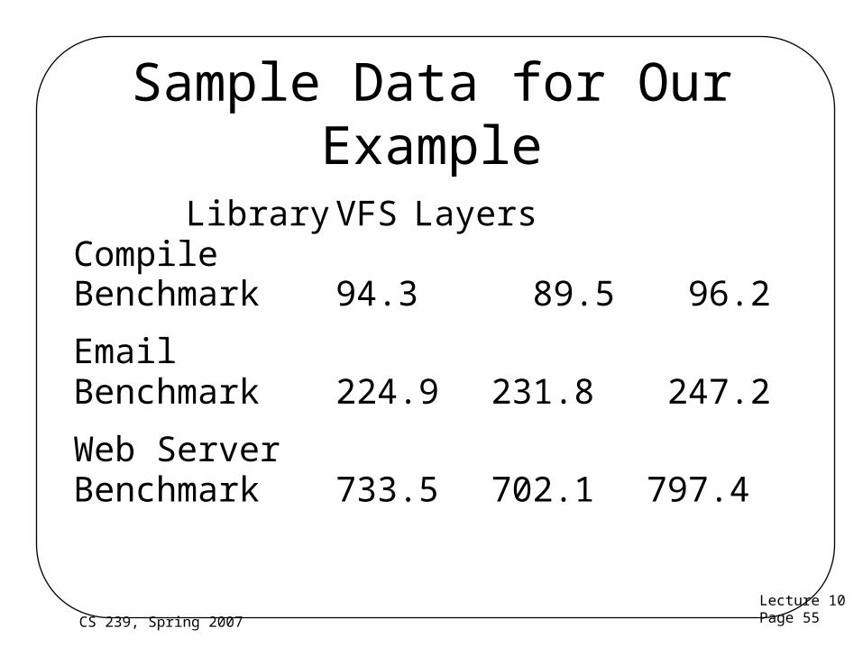
Sample Data for Our Example

Library VFSLayers

CompileBenchmark 94.3 89.5 96.2

EmailBenchmark 224.9 231.8 247.2

Web ServerBenchmark 733.5 702.1 797.4


Computing

• Averaging the jth column,

• By design, the error terms add to zero

• Also, the js add to zero, so

• Averaging rows produces

• Averaging everything produces

yb b

ej j ii

iji

. 1 1

y j j. yi i.

y..


So the Parameters Are . . .

y..

j jy y . ..

i iy y . ..


Calculating Parameters for Our Example

• = grand mean = 357.4

• j = (-6.5, -16.3, 22.8)

• i = (-264.1, -122.8, 386.9)

• So, for example, the model states that the email benchmark using a special-purpose VFS will take 357.4 - 16.3 -122.8 seconds

– Which is 218.3 seconds


Estimating Experimental Errors

• Similar to estimation of errors in previous designs

• Take the difference between the model’s predictions and the observations

• Calculate a Sum of Squared Errors

• Then allocate the variation


Allocating Variation

• Using the same kind of procedure we’ve used on other models,

• SSY = SS0 + SSA + SSB + SSE

• SST = SSY - SS0

• We can then divide the total variation between SSA, SSB, and SSE


Calculating SS0, SSA, and SSB

• a and b are the number of levels for the factors

SS ab0 2

SSA b jj

2

SSB a ii

2


Allocation of Variation For Our Example

• SSE = 2512• SSY = 1,858,390• SS0 = 1,149,827• SSA = 2489• SSB = 703,561• SST=708,562• Percent variation due to A - .35%• Percent variation due to B - 99.3%• Percent variation due to errors - .35%

So very little variation due to compression technology used


Analysis of Variation• Again, similar to previous models

– With slight modifications

• As before, use an ANOVA procedure

– With an extra row for the second factor

– And changes in degrees of freedom

• But the end steps are the same

– Compare F-computed to F-table

– Compare for each factor


Analysis of Variation for Our Example

• MSE = SSE/[(a-1)(b-1)]=2512/[(2)(2)]=628• MSA = SSA/(a-1) = 2489/2 = 1244• MSB = SSB/(b-1) = 703,561/2 = 351,780• F-computed for A = MSA/MSE = 1.98• F-computed for B = MSB/MSE = 560• The 95% F-table value for A & B = 6.94• A is not significant, B is

– Remember, significance and importance are different things


Checking Our Results With Visual Tests

• As always, check if the assumptions made by this analysis are correct

• Using the residuals vs. predicted and quantile-quantile plots


Residuals Vs. Predicted Response for Example

-30

-20

-10

0

10

20

30

40

0 100 200 300 400 500 600 700 800 900


What Does This Chart Tell Us?

• Do we or don’t we see a trend in the errors?

• Clearly they’re higher at the highest level of the predictors

• But is that alone enough to call a trend?

– Perhaps not, but we should take a close look at both the factors to see if there’s a reason to look further

– And take results with a grain of salt


Quantile-Quantile Plot for Example

-40

-30

-20

-10

0

10

20

30

40

-2 -1.5 -1 -0.5 0 0.5 1 1.5 2


Confidence Intervals for Effects

• Need to determine the standard deviation for the data as a whole

• From which standard deviations for the effects can be derived

– Using different degrees of freedom for each

• Complete table in Jain, pg. 351


Standard Deviations for Our Example

• se = 25

• Standard deviation of -

• Standard deviation of j -

• Standard deviation of i -

s s abe / / .25 3 3 8 3

s s a abj e 1 25 2 9 11 8.

s s b abi e 1 25 2 9 11 8.


Calculating Confidence Intervals for Our Example

• Just the file system alternatives shown here

• At 95% level, with 4 degrees of freedom

• CI for library solution - (-39,26)

• CI for VFS solution - (-49,16)

• CI for layered solution - (-10,55)

• So none of these solutions are 95% significantly different than the mean

Documents

Lecture 10 Page 1 CS 239, Spring 2007 Experiment Designs for Categorical Parameters CS 239 Experimental Methodologies for System Software Peter Reiher