Embed Size (px)
Citation preview

Lecture 11
Premixed Turbulent Combustion:
The Regime Diagram
11.-1
Regimes in Premixed Turbulent Combustion
Diagrams defining regimes of premixed turbulent combustion in terms of velocity and length scale ratios have been proposed by Borghi (1985), Peters (1986),Abdel-Gayed and Brandley (1989), Poinsot et al. (1990) and many others.
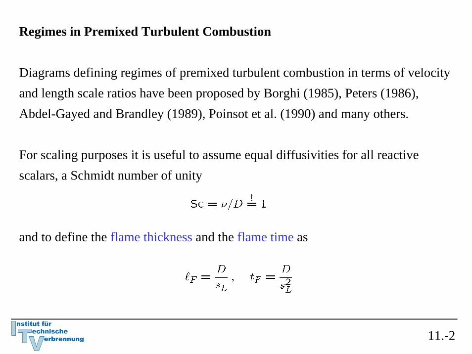
For scaling purposes it is useful to assume equal diffusivities for all reactive scalars, a Schmidt number of unity
and to define the flame thickness and the flame time as
11.-2

Then, using ν = D, the turbulent intensity and the turbulent length scale introduced in Lecture 10, we define the turbulent Reynolds number as
and the turbulent Damköhler number
Furthermore, with the Kolmogorov time, length, and velocity scales defined inLecture 10, we introduce two turbulent Karlovitz numbers.
The first one defined as
measures the ratios of the flame scales in terms of the Kolmogorov scales.
11.-3

Using the definitions
with ν = D and
taken as equality it is seen that
can be combined to show that
11.-4

Referring to the discussion about the appropriate reaction zone thickness δ in two-steps premixed flames in Lecture 6, a second Karlovitz number Kaδ may be introduced as
where for the reaction zone thickness
has been used.
11.-5

Regime diagram for premixed turbulent combustion
Using
and
where for scaling purposes we have set , such that the
Kolmogorov length scale squared becomes
the ratios may be expressed in terms of Re and Ka as
11.-6
Regime diagram for premixed turbulent combustion
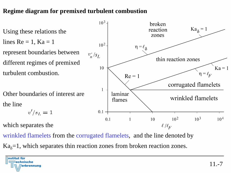
Using these relations the lines Re = 1, Ka = 1represent boundaries between different regimes of premixedturbulent combustion.
Other boundaries of interest are the line
which separates the wrinkled flamelets from the corrugated flamelets, and the line denoted byKaδ=1, which separates thin reaction zones from broken reaction zones.
11.-7

Regime diagram for premixed turbulent combustion
The line Re = 1 separates all turbulent flame regimes Characterized by Re > 1 from the regime of laminar flames (Re < 1), which is situated in the lower-left corner of the diagram.
We will consider turbulent combustion forlarge Reynolds numbers, which corresponds to a region sufficiently removed from the line Re = 1 towards the upper r.h.s.
11.-8

Regime diagram for premixed turbulent combustion
We will not consider the wrinkled flamelet regime, because it is not of much practical interest.
In that regime, where v' < sL, the turn-over velocity v' of
even the large eddies is not large enough to compete with the advancement of the flame front with the laminar burning velocity sL. Laminar flame propagation therefore is dominating over flame front corrugations by turbulence.
11.-9
Regime diagram for premixed turbulent combustion
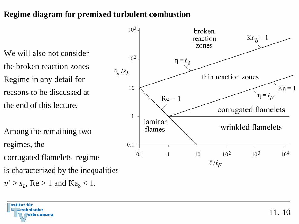
We will also not consider the broken reaction zones Regime in any detail for reasons to be discussed at the end of this lecture.
Among the remaining tworegimes, the corrugated flamelets regime is characterized by the inequalitiesv’ > sL, Re > 1 and Kaδ < 1.
11.-10

The corrugated flamelet regime
In view of
the Ka < 1 indicates that
which means that the entire reactive-diffusive flame structure of thickness is embedded within eddies of the size of the Kolmogorov scale, where the flow is quasi-laminar.
11.-11

The corrugated flamelet regime
Therefore the flame structure is not perturbed by turbulent fluctuations and remainsquasi-steady.
The boundary of the corrugated flamelets regime to the thin reaction zones regimeis given by Ka = 1, which, according to
is equivalent to the condition that the flame thickness is equal to the Kolmogorovlength scale. This is called the Klimov-Williams criterion.
11.-12

The thin reaction zones regime is characterized by Re > 1, Kaδ < 1, and Ka >1.
Ka >1 indicates that the smallest eddies of size η can enter into the reactive-diffusive flame structure since
These small eddies are still larger than the inner layer thickness
and can therefore not penetrate into that layer.
11.-13
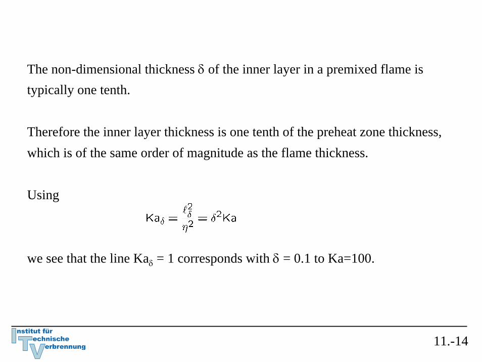
The non-dimensional thickness δ of the inner layer in a premixed flame is typically one tenth.
Therefore the inner layer thickness is one tenth of the preheat zone thickness, which is of the same order of magnitude as the flame thickness.
Using
we see that the line Kaδ = 1 corresponds with δ = 0.1 to Ka=100.
11.-14

This value is used for the upper limit of the thin reaction zones regime.
It seems roughly to agree with the flamelet boundary obtained in numerical studies, where 2D interactions between a laminar premixed flame frontand a vortex pair were analyzedPoinsot (1991).
These simulations correspond to Ka=180 for cases without heat loss and Ka=25 with small heat loss. The authors argued that since quenching by vortices occurs only for larger Karlovitz numbers, the region below the limiting value of the Karlovitz number should correspond to the flamelet regime.
11.-15

We will now enter into a more detailed discussion of the two flamelet regimes.
In the regime of corrugated flamelets there is a kinematic interactionbetween turbulent eddies and the advancing quasi-laminar flame structure.
With Ka < 1 we have:
To determine the size of the eddy that interacts locally with the flame front, we set the turn-over velocity vn = sL in
This determines the the Gibson scale (cf. Peters ,1986) as
11.-16

Eddies of the size of the Gibson scale
which have a turnover velocity vn = sL
can interact with the flame front.
Since the turn-over velocity of the large eddies is larger than the laminar burning velocity, these eddies will push the flame front around, causing a substantial corrugation.
Smaller eddies of size having a turnover velocity smaller than sL will not even be able to wrinkle the flame front.
11.-17

With
one may also write
The Gibson scale may be illustrated graphically within the inertial range.
Here, following Kolmogorov scaling in the inertial range given by
the logarithm of the velocity vn is plotted over the logarithm of the length scale .
11.-18
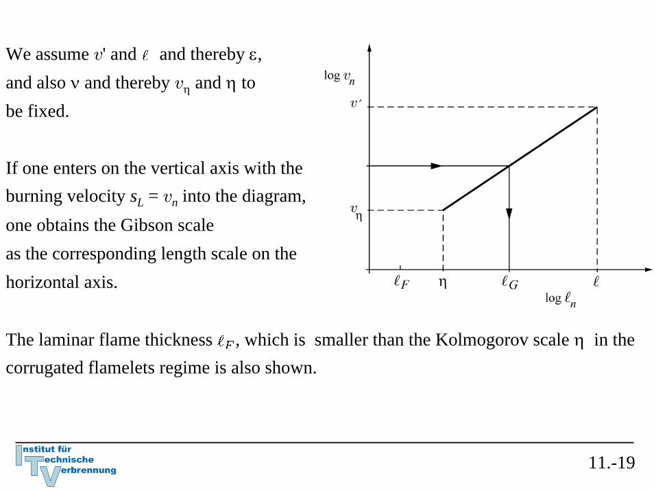
We assume v' and and thereby ε, and also ν and thereby vη and η to be fixed.
If one enters on the vertical axis with the burning velocity sL = vn into the diagram, one obtains the Gibson scaleas the corresponding length scale on the horizontal axis.
The laminar flame thickness , which is smaller than the Kolmogorov scale η in the corrugated flamelets regime is also shown.
11.-19

This diagram illustrates the limiting values of the Gibson scale:
If the burning velocity is equal to v', the Gibson scale is equal to the integral length scale:
This case corresponds to the borderline between corrugated and wrinkled flameletsin the regime diagram.
Conversely, if the burning velocity is equal to the Kolmogorov velocity, the Gibson scale is equal to the Kolmogorov scale,
which corresponds to the line Ka = 1 in the regime diagram.
11.-20

It has been shown by Peters (1992) that the Gibson scale is the lower cut-off scale of the scalar spectrum function in the corrugated flamelets regime.
At that cut-off there is only a weak change of slope in the scalar spectrum function.
This is the reason why the Gibson scale is difficult to measure.
The stronger diffusive cut-off occurs at the Obukhov-Corrsin scale defined by
Since we have assumed D = ν this scale is equal to the Kolmogorov scale.
11.-21

The next flamelet regime in the regime diagram is the regime of thin reactionzones.
As noted earlier, in the thin reaction zone regime
small eddies can enter into the preheat zone and increase scalar mixing,
However these eddies cannot penetrate into the inner layer since
The burning velocity is smaller than the Kolmogorov velocity which would lead to a Gibson scale that is smaller than the Kolmogorov scale.
11.-22

A time scale, however, can be used in the thin reaction zones regime to define acharacteristic length scale using Kolmogorov scaling in the inertial range.
That time scale should represent the response of the thin reaction zone and the surrounding diffusive layer to unsteady perturbations.
The appropriate time is the as the flame time tF.
Combining the flame time with the diffusivity D, the resulting diffusion thickness
is then of the order of the flame thickness:
11.-23

By setting tn = tF and in
one obtains the length scale
An appropriate interpretation is that of a mixing length scale, which has been advocated based on the concept of thin reaction zones by Peters (1999).
It is the size of an eddy within the inertial range which has a turnover time equal to the time needed to diffuse scalars over a distance equal to the diffusion thickness.
11.-24

During its turnover time an eddy of size will interact with the advancingreaction front and will be able to transport preheated fluid from a region of thickness
in front of the reaction zone over a distance corresponding to its own size.
Much smaller eddies will also dothis but since their size is smaller, their action will be masked by eddies of size .
Larger eddies have a longer turn-over time and would therefore be able to transport thicker structures than those of thickness . They will therefore corrugate the broadened flame structure at scales larger than .
11.-25
The physical interpretation of is therefore that of the maximum distance that preheated fluid can be transported ahead of the flame.
As a mixing length scale had already been identified by Zimont (1979).
Differently from the Gibson length scale the mixing length scale can beobserved experimentally.
Changes of the instantaneous flame structure with increasing Karlovitz numbers have been measured by Buschmann et al. (1996) who used 2D-Rayleigh thermometry combined with 2D laser-induced fluorescence on a turbulent premixedBunsen flame.
They varied the Karlovitz number between 0.03 and 13.6 and observed at Ka > 5 thermal thicknesses that largely exceed the size of the smallest eddies in the flow.
11.-26

The mixing scale may be illustrated in a log-log plot of tn over .
If one enters the time axis at tF = tn, the mixing length scaleon the length scale axis is obtained.
If tF is equal to the Kolmogorov time tη, the mixing length is equal to theKolmogorov scale.
In this case, one obtains at the border between the thin reaction zones regime and the corrugated flameletsregime.
11.-27

Similarly, if the flame time is equal to the integral time
the mixing length is equal to the integral length scale.
This corresponds to Da = 1, which Borghi (1985) interpreted as theborderline between two regimes in turbulent combustion.
However, it merely sets a limit for the mixing scale which cannot increase beyond the integral scale.
11.-28

The diffusion thickness
is also indicated.
There also appears the Obukhov-Corrsin scale, which is the lower cut-off scale of the scalar spectrum in the thin reaction zones regime.
Since we have assumed ν = D, the Obukhov-Corrsin scale is equal to the Kolmogorovlength scale:
11.-29
As a final remark related to the corrugated flamelets regime and the thin reaction zones regime, it is important to realize that turbulence in high Reynolds number turbulence is intermittent and the dissipation ε has a statistical distribution.
This refinement of Kolmogorov's theory has led to the notion of intermittency or"spottiness" of the activity of turbulence in a flow field, Monin and Yaglom (1975) .
This may have important consequences on the physical appearance of turbulent flames at sufficiently large Reynolds numbers.
One may expect that the flame front shows manifestations of strong local mixing by small eddies as in the thin reaction zones regime as well as rather smooth regions where corrugated flamelets appear. The two regimes discussed above may therefore both be apparent in the same experimentally observed turbulent flame.
11.-30

Beyond the line Kaδ = 1 there is a regime called the broken reaction zones regime where Kolmogorov eddies are smaller than the inner layer thickness .
They may therefore enter into the inner layer and perturb it with the consequence that chemistry breaks down locally due to enhanced heat loss to the preheat zone followed by temperature decrease and the loss of radicals.
When this happens the flame will extinguish and fuel and oxidizer will interdiffuseand mix at lower temperatures where combustion reactions have ceased.
In a series of papers Mansour et al. (1992), Chen et al. (1996),Chen and Mansour (1997) and Mansour et al. (1998) have investigated highly stretched premixed flames on a Bunsen burner which were surrounded by a large pilot.
11.-31

11.-32
Simultaneous temperature and CH measurements
They found a thin reaction zone, as deduced from the CH profile, and steep temperature gradients in the vicinity of that zone.
There also was evidence of occasional extinction of the reaction zone.
This corresponds to instantaneous shots where the CH profile was absentas in the picture on the upper r.h.s. Such extinction events do not occur in the flame F3 which has a Karlovitz number of 23 and is located in the middle of the thin reaction zones regime.
It can be expected that local extinction events would appear more frequently, if the exit velocity is increased and the flame enters into the broken reaction zones regime.
11.-33

Local extinction events will occur at an exit velocity close to 75m/s so frequently that the entire flame extinguishes.
Therefore one may conclude that inthe broken reaction zones regime a premixed flame is unable to survive.
The measurements also show strong perturbations of the temperature profile on the unburnt side of the reaction zone.
This is most evident in the picture on the lower l.h.s., where the temperature reaches more than 1100 K but falls back to 800 K again.
This seems to be due to small eddies that enter into the preheat zone and confirms the concept of the thin reaction zones regime.
11.-34

Regimes in Premixed Combustion LES
A similar regime diagram can be constructed for LES using the filter size Δ as the length scale and the subfilter velocity fluctuation v'Δ as the velocity scale.
Such a representation introduces both physical and modeling parametersinto the diagram. A change in the filter size, however, also leads to a change in the subfilter velocity fluctuation. This implies that the effect of the filter size, which is a numerical or model parameter, cannot be studied independently.
In response to this issue, an LES regime diagram for characterizing subfilterturbulence/flame interactions in premixed turbulent combustion was proposed by Pitsch & Duchamp de Lageneste (2002), and was recently extended by Pitsch (2005).
11.-35

11.-36
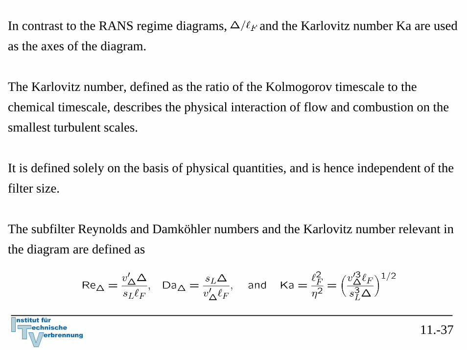
In contrast to the RANS regime diagrams, and the Karlovitz number Ka are used as the axes of the diagram.
The Karlovitz number, defined as the ratio of the Kolmogorov timescale to the chemical timescale, describes the physical interaction of flow and combustion on the smallest turbulent scales.
It is defined solely on the basis of physical quantities, and is hence independent of the filter size.
The subfilter Reynolds and Damköhler numbers and the Karlovitz number relevant in the diagram are defined as
11.-37

In LES, the Karlovitz number is a fluctuating quantity, but for a given flow fieldand chemistry it is fixed.
The effect of changes in filter size can therefore easily be assessed at constant Ka number.
An additional benefit of this regime diagram is that it can be used equally well for DNS if Δ is associated with the mesh size.
In the following, the physical regimes are briefly reviewed and relevant issues for LES are discussed.
11.-38

The effect of changing the LES filter width can be assessed by starting from any oneof these regimes at large ratios
As the filter width is decreased, the subfilter Reynolds number, ReΔ, eventually becomes smaller than one.
Then the filter size is smaller than the Kolmogorov scale, and no subfilter modeling for the turbulence is required.
However, the entire flame including the reaction zone is only resolved if Δ < δ.
11.-39

In the corrugated flamelets regime, if the filter is decreased below the Gibson scale,
which is the smallest scale of the subfilter flame-front wrinkling, the flame-front wrinkling is completelyresolved.
It is apparent that in the corrugated flamelet regime, where the flame structure is laminar, the entire flame remains on the subfilter scale, if
This is always the case for LES.
11.-40
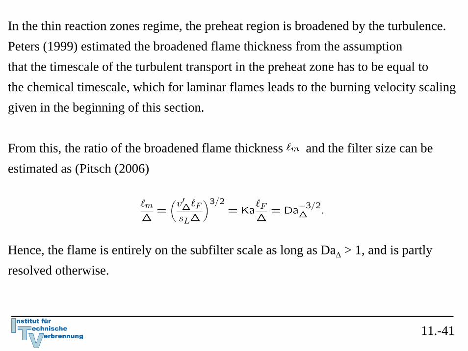
In the thin reaction zones regime, the preheat region is broadened by the turbulence.Peters (1999) estimated the broadened flame thickness from the assumptionthat the timescale of the turbulent transport in the preheat zone has to be equal tothe chemical timescale, which for laminar flames leads to the burning velocity scalinggiven in the beginning of this section.
From this, the ratio of the broadened flame thickness and the filter size can be estimated as (Pitsch (2006)
Hence, the flame is entirely on the subfilter scale as long as DaΔ > 1, and is partlyresolved otherwise.
11.-41

It is important to realize that the turbulence quantities, especially v'Δ, and hencemost of the nondimensional numbers used to characterize the flame/turbulence interactions, are fluctuating quantities and can significantly change in space and time.
To give an example, the variation of these quantities from a specific turbulent stoichiometric premixed methane/air flame simulation is shown in the regime diagram.
This simulation was done for an experimental configuration with a nominal Karlowitz number of Ka = 11, based on experimentally observed integral scales.
The simulated conditions correspond to flame F3 of Chen et al. (1996), and details of the simulation can be found in Pitsch & Duchamp de Lageneste (2002).
11.-42

11.-43
Appendix
A

Therefore the flame structure is not perturbed by turbulent fluctuations and remains quasi-steady.
The boundary of the corrugated flamelets regime to the thin reaction zones regimeis given by Ka = 1, which, according to
is equivalent to the condition that theflame thickness is equal to the Kolmogorov length scale:This is called the Klimov-Williams criterion.
For Ka = 1 the flame time is equal to the Kolmogorov time and the burning velocity is equal to the Kolmogorov velocity.
11.-13

Among the flames F1, F2 and F3 that were investigated, the flame F1 with an exit velocity of 65 m/s was close to total flame extinction which occured on this burner at 75 m/s.
A photograph of the flame is shown in Chen et al. (1996).
Mansour (1999) has reviewed the recent results obtained from laser-diagnostics applied to turbulent premixed and partially premixed flames.
Mansour et al. (1998) have shown that the flame F1 is on the borderline to the broken flamelets regime having a Karlovitz number of Ka=91.
11.-32

The three regimes with essentially different interactions of turbulence andchemistry are the corrugated flamelet regime, the thin reaction zones regime, andthe broken reaction zones regime.
In the corrugated flamelet regime, the laminar flame thickness is smaller than the Kolmogorov scale, and hence Ka < 1.
Turbulence will therefore wrinkle the flame, but will not disturb the laminar flame structure.
In the thin reaction zones regime, the Kolmorogov scale becomes smaller than the flame thickness, which implies Ka > 1.
Turbulence then increases the transport within the chemically inert preheat region.
11.-41

In thin reaction zones regime, the reaction zone thickness is still smaller than the Kolmogorov scale:
Because the reaction zone, which appears as a thin layer within the flame, can be estimated to be an order of magnitude smaller than the flame thickness, the transition to the broken reaction zones regime occurs at approximately
The thin reaction zone retains a laminar structure in the thin reaction zones regime, whereas the preheat region is governed by turbulent mixing, which enhances the burning velocity.
11.-42

In the broken reaction zones regime, the Kolmogorov scale becomes smaller than the reaction zone thickness:
This implies that the Karlovitz number Kaδ , based on the reaction zone thickness, becomes larger than one.
Most technical combustion devices are operated in the thin reaction zones regime,because mixing is enhanced at higher Ka numbers, which leads to higher volumetricheat release and shorter combustion times.
The broken reaction zones regime is usually avoided in fully premixed systems.
11.-43
In the broken reaction zones regime , mixing is faster than the chemistry, which leads to local extinction. This can cause noise, instabilities, and possibly global extinction.
However, the broken reaction zones regime is significant, for instance, in partially premixed systems.
In a lifted jet diffusion flame, the stabilization occurs by partially premixed flame fronts, which burn fastest at conditions close to stoichiometric mixture.
Away from the stoichiometric surface toward the center of the jet, the mixture is typically very rich and the chemistry slow. Hence, the Ka number becomes large. This behavior has been found in the analysis of DNS results of a lifted hydrogen/air diffusion flame (Mizobuchi et al. 2002).
11.-44

For a given point in time, the Ka number has been evaluated using appropriate subfilter models for all points on the flame surface.
Because of the spatially varying filter size, but also because of heat losses to theburner, which locally lead to changes in the flame thickness, there is a small scatter of the dimensionless filter width.
Although the flame is mostly in the thin reaction zones regime, there is a strong variation in Ka number, ranging from the corrugated to the broken reaction zones regime.
11.-49